Applying Machine Learning in Retail Demand Prediction—A Comparison of Tree-Based Ensembles and Long Short-Term Memory-Based Deep Learning

Abstract

In the realm of retail supply chain management, accurate forecasting is paramount for informed decision making, as it directly impacts business operations and profitability. This study delves into the application of tree-based ensemble forecasting, specifically using extra tree Regressors (ETRs) and long short-term memory (LSTM) networks. Utilizing over six years of historical demand data from a prominent retail entity, the dataset encompasses daily demand metrics for more than 330 products, totaling 5.2 million records. Additionally, external variables, such as meteorological and COVID-19-related data, are integrated into the analysis. Our evaluation, spanning three perishable product categories, reveals that the ETR model outperforms LSTM in metrics including MAPE, MAE, RMSE, and R². This disparity in performance is particularly pronounced for fresh meat products, whereas it is marginal for fruit products. These ETR results were evaluated alongside three other tree-based ensemble methods, namely XGBoost, Random Forest Regression (RFR), and Gradient Boosting Regression (GBR). The comparable performance across these four tree-based ensemble techniques serves to reinforce their comparative analysis with LSTM-based deep learning models. Our findings pave the way for future studies to assess the comparative efficacy of tree-based ensembles and deep learning techniques across varying forecasting horizons, such as short-, medium-, and long-term predictions.

1. Introduction

Forecasting remains at the forefront of decision making [1,2], especially in the field of supply chain management where accurate predictions of demand and inventory levels can have a significant impact on business operations and profitability [3,4]. Forecasting methodologies and algorithms to predict more accurate results have been developed throughout the ages [5]. In retail, rapid changes to the business environment, shorter planning horizons, lower profit margins, and customer service issues make forecasting more complex [6]. In addition, large numbers of product types compel businesses to adopt individual models for specific groups of products, covering linear to complex nonlinear patterns [7]. Global uncertainty and the plethora of complexities in the retail industry make forecasting accuracy one of the main priorities in this field.

Recently, researchers have utilized advanced methods of forecasting, such as deep neural networks, like long short-term memory (LSTM) or ensemble learning, to increase accuracy. Ensemble techniques combine different algorithms into an individual method, where each algorithm could be more sensitive under varying conditions [8]. Combined forecasts or “ensemble forecasts” have historical roots in aggregating individual forecasts and are not a recent development. However, using them in machine learning models has recently gained increasing popularity in the field of applied artificial intelligence in business. More than 15% of forecasting research in 2021 mentioned combined machine learning models [9]. Numerous combination and ensemble techniques have been developed to improve forecasting accuracy. Among the different machine learning models, tree-based methods dominate in both accuracy and uncertainty handling [10]. Compared to other machine learning algorithms, tree-based models have relatively low requirements for data preparation tasks, like feature scaling [11]. Extra tree regression (ETR), which is a type of tree-based ensemble model, has gained popularity in predictive research due to its ability to learn faster with smaller input dimensions [12]. Ensemble forecasting is also utilized in the retail sector to overcome uncertainties in data, parameters, and models and to decrease the risks of relying on a single best model. However, the usage of ensemble models in retail prediction has not been widely investigated in the research [7].

To address this research gap, this paper aims to perform tree-based ensemble demand forecasting alongside deep learning with LSTM networks. To fulfill this objective, this study utilizes real-life data from a large-scale research project in retail supply chain management, comprising over 5.2 million records. More precisely, we utilize data from a prominent Austrian retailer, including daily demand data for over 330 products. The retail company has been a partner of a 4-year research project focusing on improving demand prediction for perishable food in grocery retail by means of advanced analytics. To compare the results of both approaches and determine the most effective one, the methodology of this paper builds on an acknowledged set of model evaluation criteria. The contributions of our paper that distinguish our work from previous studies can be summarized as follows:

• Feature diversity: Our study goes beyond historical demand data by incorporating a wide array of diverse features, including price and external factors, such as weather and COVID-19-related data. This enriched dataset enhances our understanding of demand behavior;
• Real-world applicability: We utilize a substantial dataset from a prominent supermarket, demonstrating the real-world applicability of our findings. This authenticity adds credibility to our research and enhances its practical relevance;
• Advanced machine learning models: We leverage advanced machine learning techniques by employing two state-of-the-art models selected for their ability to handle complex datasets and capture intricate demand patterns effectively to improve forecast accuracy in an uncertain environment;
• Category-based analysis: To comprehensively evaluate our forecasting models, we conduct category-based analyses across three distinct perishable product categories. This approach showcases the models’ effectiveness in handling diverse consumer behaviors and demand patterns.

The remainder of the paper is structured as follows. Section 2 presents the findings of a comprehensive literature review on the use of ensemble methods in different domains. Section 3 outlines the methodology of the study, including data source, cleaning, preparation, and modeling steps. Section 4 evaluates the demand forecasting results of two chosen methods and compares their performance in predicting demand for three product groups. Finally, Section 5 concludes the paper and offers insights for future research.

2. Background

Traditional machine learning techniques used for forecasting can be categorized into three main groups: (1) time series analysis, (2) regression-based approaches, and (3) supervised and unsupervised methods [13]. Time series analysis methods are the most widely used, encompassing techniques like autoregressive integrated moving average (ARIMA) and Holt Winter Exponential Smoothing (HW). These methods, particularly in the context of retail demand forecasting, are highly regarded for their ability to capture trends and seasonal demand patterns [14,15]. Regression-based methods have the flexibility to consider both independent and dependent variables [5]. And third, supervised and unsupervised models, like artificial neural networks (ANNs) or long short-term memory (LSTM), have been shown to perform better in nonlinear data [16]. The utilization of advanced models in forecasting has experienced growth in various industries, including oil, food and agriculture, public transportation, and retail. The performance of these models has been investigated in these industries, and it was found that ensemble models could outperform other models regarding accuracy [17,18,19].

To gain a deeper understanding of the application of advanced algorithms in demand forecasting, we have conducted a search using the keywords “demand forecasting” and “ensemble” in online databases focusing on recent years. We found a significant number of studies that have used advanced machine learning approaches in the field of energy. For instance, Yu et al. (2016) proposed a new method for predicting crude oil prices using an ensemble empirical mode decomposition (EEMD) and extended extreme learning machine (EELM) to forecast electricity load [20]. Ribeiro et al. (2019) have presented a framework for short-term load forecasting using the Wavenet ensemble [21]. The framework involves transforming the data, determining an optimal time window, and selecting features. The proposed framework outperforms existing similar forecasting techniques, like multilayer perceptron neural networks. In electricity price forecasting, Zhang et al. (2022) introduced a hybrid deep neural network approach, which utilizes the Catboost algorithm for feature selection and a bidirectional long short-term memory neural network (BDLSTM) as the main forecasting engine [22]. In a recent study, Da Silva et al. (2021) proposed a new method for short-term prediction in microgrids called the Ensemble Prediction Network (EPN). The EPN comprises an ensemble of nine linear predictive nodes and is designed to provide an optimal estimate of predicted demand through least-squares optimization under certain constraints [23]. To overcome uncertainty, Yang et al. (2017) used combination approaches in a HAR model that considers lags of realized volatility and other potential predictors [24]. In the tourism industry, Cankurt (2016) developed and implemented ensemble learners for tourism demand forecasting based on M5P and M5-Rule model trees and random forest algorithms. The learners were evaluated using bagging, boosting, randomization, stacking, and voting techniques for forecasting tourism demand in Turkey [17]. Ensemble models have also been applied in public transportation, where Dai et al. (2018) presented a data-driven framework for short-term metro passenger flow prediction that utilizes both spatial and temporal information. The passenger flow information is obtained from smart-card data, and passenger flow patterns are explored. The proposed framework consists of two basic prediction models and a probabilistic model selection method (random forest classification) to combine the outputs for better prediction [25]. In an agricultural application field, Ribeiro and dos Santos Coelho (2020) investigated the accuracy of forecasting agricultural commodity prices through regression ensembles. The aim of their study was to compare the performance of ensembles (bagging, boosting, and stacking) with reference models such as support vector machine (SVR), multilayer perceptron (MLP), and K-nearest neighbor (KNN) in forecasting prices one month ahead. Their study used monthly time series data for the price of soybean and wheat in the state of Parana, Brazil [26]. In the steel industry, Raju et al. (2022) compared the performance of different machine learning models for demand forecasting in the steel industry. Their study found that the best results came from a combination of models called STACK1 (extreme learning machine + gradient boosting + XGBR-SVR [27].

In the retail industry, a new heuristic approach was applied in a Turkish retail chain (SOK Market) with 4000 stores and 1500 SKUs. The results led to a reduction in stock outs, increased revenue by 30%, a 10% decrease in stock days, and a 34% reduction in waste for perishable products [8]. Das Adhikari et al. (2017) introduced a new ensemble technique using an averaging method that prioritizes algorithms with good accuracy and reduces deviation from actual sales. The method gives importance to algorithms that perform well based on historical data and penalizes those that deviate from actual sales [28]. Wang et al. (2018) applied ensemble empirical mode decomposition (EEMD) for global food price volatility and decomposed the original food price series into intrinsic mode functions and a residual. In their study, they mentioned that the low-frequency component contributes more to food price volatility, which is caused by notable events and policies. High-frequency components are mainly influenced by small events and market adjustments in a time series analysis. In the long term, food prices are determined by an intrinsic trend from global economic development. The findings reveal that food price volatility is a complex issue with multiple factors affecting both low and high frequencies [29]. In another study, daily optimal ordering quantities of fresh products using six methodologies (LSTM, SVR, RFR, GBR, XGBoost, and ARIMA) were analyzed. The paper compared the performance of conventional statistics, like ARIMA, and various machine learning algorithms, including RNNs (LSTM), SVRs, decision trees/ensemble methods (RFRs), and boosted trees (GBR, XGBoost). It was found that the LSTM and SVR machine learning algorithms outperformed the other demand forecasting models for the dataset [30].

Arora et al. (2020) focused on forecasting sales demand using historical data from a wholesale alcoholic beverage distributor. They employed an ensemble approach by combining traditional statistical models, multivariate models, and deep learning models. The study showed a reduction in the sale forecasting error by almost 50% and 33.5% for the most sold and highest revenue-grossing products respectively, compared to a naive model. The authors concluded that each product needs a unique model for accurate demand forecasting [31]. Sharma and Omair Shafiq (2020) used historical retail purchase data to predict the probability of item purchases. An ensemble learning model was built using random forests (RFs), Convolutional Neural Networks (CNNs), Extreme Gradient Boosting (XGBoost), and a voting mechanism. The model was evaluated using metrics such as accuracy, precision, F1 score, sensitivity, and specificity, and they experienced better performance using ensemble models than existing solutions [32].

Zhang et al. (2022) aimed to forecast weekly retail sales using Walmart’s retail data from over five years. The forecast subject was divided into twenty-one time series based on different departments and states. Four machine learning models (naïve, moving average, prophet, ETS) were used to train the data, and stacking was used as the ensemble technique. The results showed that while the ensemble model using linear regression performed the best in the validation stage, the weighted average method supported by random forests was the best in the testing stage. Linear regression was found to be overfitting. The research concluded that ensemble learning, especially weighted average, was a recommended method for forecasting [33]. Another previous study examined data mining’s role in predicting retail sales for Walmart’s outlets using supervised machine learning techniques. By analyzing factors like past sales, promotions, holidays, and economic indicators, the research helps businesses optimize sales forecasts and marketing strategies. The results suggest that simple regression techniques might not be optimal for short-term sales prediction with limited historical data. Ensemble learning techniques, involving the averaging of results from multiple decision trees, show better accuracy. Thus, for such scenarios, business owners are advised to opt for ensemble learning models [34]. Seyedan et al. (2022) proposed a demand forecasting methodology for the sports retail industry using ensemble learning. The methodology includes a cluster-based demand prediction using the time-series forecasting methods LSTM and prophet and majority voting and BMA as ensemble learning techniques. The aim was to improve the accuracy of future daily demand forecasting by combining different models and assigning higher weights to better-performing models. The results show that the clustered–ensembled approach improves prediction accuracy compared to using single models, leading to minimum values of MAPE, MAE, and RMSE. Their proposed framework had a considerable increase in prediction accuracy in various seasonal and monthly cases [18]. Ma et al. (2022) introduced a Spatial–Temporal Graph Attentional LSTM (STGA-LSTM) neural network for predicting short-term bike sharing demand utilizing various data sources. This model outperforms baseline approaches, leveraging deep learning to capture spatiotemporal patterns in bike sharing systems [35].

Table 1. Overview of selected previous works.

Publication	Year	Domain	Ensemble Algorithms	Features
[20]	2016	Crude oil price forecasting	EEMD and EELM
[17]	2016	Tourism demand forecasting	Bagging, boosting, randomization, and stacking
[8]	2017	Retail demand forecasting	Boosting	Daily sale, special days, and promotion days
[28]	2017	Supply chain demand forecasting	Averaging ensemble model
[24]	2017	Agriculture commodities forecasting	Bagging
[36]	2017	Hog price forecasting	EEMD
[25]	2018	Metro passenger flow forecasting	Averaging ensemble model	Eight neighboring origin–destination (OD) flows are utilized as features for a single target OD flow
[29]	2018	Food price volatility forecasting	EEMD
[30]	2019	Retail demand forecasting	Bagging (RFR) and boosting (GBR and XGBR)	Daily sales
[21]	2019	Electricity load time series forecasting	.
[37]	2020	Energy load forecasting	ETB	Hour, DayOfWeek, IsWorking, Dewpnt, Drybulb, prior 1 h, prior 1 day, prior 1 week, and season
[31]	2020	Wholesale distribution demand forecasting	Weighted and non-weighted, depending on product	Monthly sales, product type, local weather, price promotions, marketing campaigns, holidays, and special events
[32]	2020	Retail purchase probability forecasting	RF, CNN, XGBoost, and voting classifier	Transactional data and newly generated features
[22]	2022	Electricity price forecasting	CatBoost	Hourly electricity price, hour of the day, weekend (the current day is weekend or not), and the day name
[26]	2020	Agribusiness prediction	Bagging (RFR), boosting (GBR and XGBR), and stacking (STACK)
[38]	2021	Food and raw materials in restaurant forecasting	Stacking	Independent variables (year, month, date, day, weather conditions, public holidays, and festive season). Dependent variables (chicken niryani, mutton biryani, dal tadka, paneer lababdar, and curd rice)
[34]	2021	Retail demand forecasting	Extra tree regression	Date, weekly sales, holiday, temperature, fuel price, CPI, and unemployment
[33]	2022	Retail demand forecasting	Stacking	State, weekly sales, price
[27]	2022	Steel demand forecasting	Bagging (RFR), boosting (GBR and XGBR), and stacking (STACK)	Availability, raw materials, workers, working days, holidays, down time, and demand level
[18]	2022	Retail demand forecasting	Majority voting	Fifty-two features related to stores, customers, products, sales, orders, shipping, and delivery

provides a summary of selected previous works, focusing on the application domain, ensemble algorithms applied, and features used.

These models, showcased through studies ranging from predicting oil prices and electricity load to optimizing passenger flow and commodity prices, consistently demonstrate superior accuracy and performance compared to traditional methods. This trend extends to retail, where ensemble approaches have led to reduced stock outs, increased revenue, and enhanced sales forecasting precision. The remarkable versatility and success of these models across various sectors highlight their potential to reshape and refine demand forecasting practices, ultimately leading to more informed and effective decision-making processes.

3. Research Methodology

The aim of this paper is to perform demand forecasting for a supermarket located in Austria by building two machine learning models and evaluating their accuracy by comparing the results. Our problem is a supervised regression machine learning problem, and we will concentrate on forecasting the demand for day $t$ based on the historical data up to day $t-1$ and other relevant data available at day $t$. The analysis will be performed at the product category level, with a focus on three product categories (A, B, and C). The first model is a tree-based ensemble model, and the second is a deep learning model with long short-term memory (LSTM) networks. For convenience, we will refer to the first model as ETR and the second model as DL. The demand forecasting process is shown in Figure 1.

Subsequently, each step is described in more detail.

3.1. Initial Dataset

Our initial dataset consists of three distinct components:

(i)

Historical demand data: Our dataset comprises historical demand data, which is also our target variable, covering a 76-month period from January 2016 to February 2022. It includes daily demand amounts for over 330 products across 3 main product categories: fruits (A), fresh meat (B), and soft drinks (C). In total, the dataset spans more than 6 years, resulting in over 5.2 million available records for training and testing. The data are extracted from a sales transaction dataset from a supermarket located in Austria;

(ii)

Internal data: This component includes data that results from business decisions, such as pricing and promotions. Key components of these internal data include pricing information and promotional activities. This dataset includes daily price values for each product;

(iii)

External data: In addition to internal factors, our dataset incorporates external variables that are beyond the direct control of the retail company. These external variables encompass various factors, including calendar-related data, weather conditions, and COVID-19-related data. Calendar-related data provide information for each day, including the month of the year, week of the year, day of the week, day of the month, and any special day or event. Weather data include temperature in Celsius, wind speed in m/s, amount of precipitation in mm, and precipitation type (no precipitation, rain, snow, rain–snow). COVID-19-related data include information about the type of lockdown, including no lockdown and lockdown.

3.2. Data Preparation

This step mostly covers all activities that involve the construction of the final dataset that will be fed into the modeling part from the initial datasets. The tasks include selecting the tables, records, and attributes, as well as transforming, cleaning, and mapping the data.

3.3. Feature Creation

In this step, features are created and extracted from the existing data attributes and transformed into a standard input dataset that can be utilized for the next steps. The creation of these features is based on prior research [8,30,33], business insights, and experience. The created features are shown in

Table 2. Created features.

Feature	Type
Demand value $(t-1,t-2,\dots ,t-24)$	Numeric
Price value $(t,t-1,\dots ,t-24)$	Numeric
Month of the year $\left(t\right)$	Categorical–Nominal
Week of the year $\left(t\right)$	Categorical–Nominal
Day of the week $\left(t\right)$	Categorical–Nominal
Day of month $\left(t\right)$	Categorical–Nominal
Special day status $\left(t\right)$	Categorical–Nominal
Day after status $\left(t\right)$	Categorical–Nominal
Day before status $\left(t\right)$	Categorical–Nominal
COVID-19 lockdown type $\left(t\right)$	Categorical–Nominal
Temperature $\left(t\right)$	Numeric
Wind speed $\left(t\right)$	Numeric
Precipitation $\left(t\right)$	Numeric
Precipitation type $\left(t\right)$	Categorical–Nominal

.

Lagged features, such as the demand from the previous day or week, are also created in this step. In our case, there are six working days, and lagged features for demand and price have been created for the previous four weeks, which are labeled $(t-1, t-2,\dots , t-24)$ in Table 2. The rest of the features only require current values, which are labeled $\left(t\right)$.

3.4. Input Dataset

The input dataset holds all the features created in the previous step, along with the target variable (demand value at day t), will be used in the next steps for feeding into the model-building process. The input dataset is split into two parts: (i) the training dataset, which includes almost 80% of the data from January 2016 to December 2020 and is used for building the models (aggregating around 4.1 million records), and (ii) the test dataset, which covers the remaining period from January 2021 to February 2022 (aggregating around 1.1 million records) and is held out and will be used for the final evaluation step as unseen data in the models.

3.5. Feature Scaling and Encoding

In this step, depending on the type of model being used, we may need to scale our numeric features and encode our categorical features in a format that can be utilized in the model training process. One advantage of tree-based models is that they do not require feature scaling [11]. Therefore, numeric features are only scaled for the DL model using Max-Min normalization. To handle categorical features, we utilized one-hot encoding to transform them (e.g., day status and precipitation type).

3.6. Feature Selection

The objective of this step is to select features from the input dataset and choose the optimal combination that produces the best results for each model. Various methods can be employed to achieve this objective. One such method involves using feature importance scores, which assign scores to each feature, prioritizing their contribution to the prediction [36,37,38]. In this study, we employ a feature importance technique based on tree-based ensembles [39]. Feature importance is measured by the extent of error reduction (such as MAE or RMSE) that each feature contributes [40]. To accomplish this, we utilize the feature importance based on decision trees available in the Python scikit-learn library [41] to identify the most suitable features for the model. Finding the optimal sliding window for using lagged features in the models is an important task of this step. For each model, the best sliding window was determined to be 6 days, meaning that lagged data from the previous 6 days will be used.

3.7. Model Training

In this step, the model is fed with features from a training dataset. The model uses these data to learn and estimate the parameters of the model through optimization with the objective of reducing errors and improving the generalization of the representations learned from the data. During this step, the machine learning algorithm adjusts the model parameters iteratively based on the training data, attempting to minimize the difference between the model’s forecasting and the true target values. In this research, we attempt to use two different models.

3.7.1. Model 1—Extra Tree Regressor (ETR)

In this model, we aim to design a tree-based ensemble model based on the bagging algorithm, which is an ensemble technique that combines the results of a large number of decision trees to produce a single forecasting. To accomplish this, we utilized the Extremely Randomized Tree (ERT) method [42]. The ERT constructs multiple decision trees by selecting random subsets of features and making random splits at each node. Unlike random forests, the ERT does not search for the best split; instead, it selects the splits randomly. This approach is particularly useful for forecasting tasks and has strength in accuracy and computational efficiency compared to other similar algorithms, such as random forest [42,43]. In this work, we implemented the Extremely Randomized Tree using the extra tree regressor model from the ensemble module of the Python scikit-learn library [41].

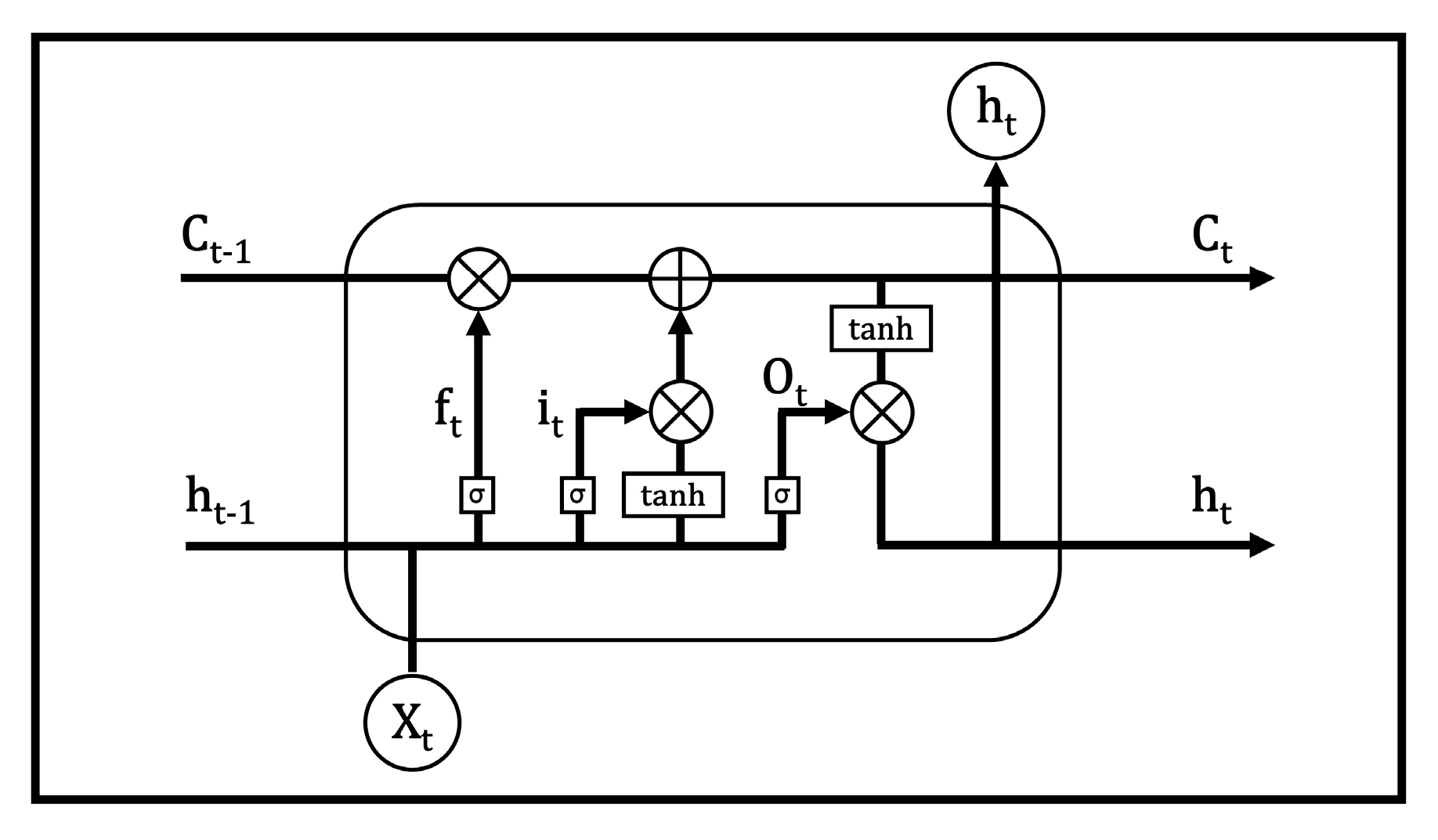
3.7.2. Model 2—LSTM-Based Deep Learning (DL)

In this model, our aim is to design a neural network that allows us to consider both lagged features and other related features in one deep learning model. To achieve this, we propose a neural network model that includes both LSTM and dense layers. This model was implemented in Python using Tensorflow and Keras [44]. The description of the primary components of our proposed deep learning model is as follows.

LSTM layer: LSTM is a special type of recurrent neural network (RNN) that is first introduced by Hochreiter and Schmidhuber (1997). It offers powerful capabilities for capturing complex temporal patterns and has become a valuable tool for time series forecasting due to its ability to capture intricate temporal patterns. LSTM learns from a sequence of data points by constructing a mathematical model that represents the relationships within the input sequence. It evaluates the data at each point in the sequence, processes them, updates their internal state, and subsequently progresses to the next time step) [45]. The LSTM architecture is illustrated in Figure 2. In this architecture, $f_t$ represents a forget gate, $i_t$ is an input gate, $o_t$ stands for an output gate, $c_t$ denotes a cell state, and $h_t$ signifies a hidden state. The simplified forms of the equations are described in Equation (1).

$$\begin{array}{c}{f}_t={\sigma }_g\left(W_f{x}_t+U_f{h}_{t-1}+b_f\right)\\ i_t={\sigma }_g\left(W_i{x}_t+U_i{h}_{t-1}+b_i\right)\\ o_t={\sigma }_g\left(W_o{x}_t+U_o{h}_{t-1}+b_o\right)\\ c_t=f_t\odot c_{t-1}+i_t\odot {\sigma }_c\left(W_c{x}_t+U_c{h}_{t-1}+b_c\right)\\ h_t=o_t\odot {\sigma }_h\left(c_t\right)\end{array}$$

(1)

where σ is an activation function and the operator ⊙ denotes the Hadamard product.

Dense layer: A dense layer, also known as a fully connected layer, is a fundamental component of neural networks. It connects every neuron from one layer to all neurons in the next layer, with each connection having a weight learned during training. The operation of a dense layer includes multiplying input values from the previous layer by their corresponding weights, summing these weighted inputs for each neuron, and optionally adding a bias term. An activation function is applied to the output of each neuron in a dense layer, introducing nonlinearity to the neural network and enabling it to capture complex, nonlinear data relationships.

3.8. Model Evaluation and Tuning

In this step, we aim to evaluate the trained model based on its input features and optimize its hyperparameters. This is performed by iteratively adjusting the inputs and hyperparameters until the best results are achieved. We aimed to find the optimal attributes for each model, such as the number of trees and the maximum depth of the trees for the ETR model, and the network configuration, activation function, learning rate, batch size, and number of epochs for the DL model. These hyperparameter tuning tasks are carried out using random search techniques and were implemented using the scikit-learn library in Python.

3.9. Trained Model

The output of the previous steps is the best model with optimized parameters on the training dataset, which is designed to generalize to new data. We use this trained model to make forecasting on unseen data (test dataset) and evaluate its performance for the final comparison. The best-trained model for the ETR and DL models was trained with the following setup.

3.9.1. Model 1—ETR

This model was trained with the mean squared error (MSE) as the function for measuring the quality of a split (criterion = mse) with 300 trees in the forest (n_estimators = 300), each tree having a maximum depth of 100 (max_depth = 100). The maximum number of features considered for each split was 50 percent of the total number of features in the dataset (max_features = 0.5). The minimum number of samples required to split an internal node was set at 10 (min_samples_split = 10), and the minimum number of samples required to be at a leaf node was set at 2 (min_samples_leaf = 2).

3.9.2. Model 2—DL

In this model, the lagged features (historical demand and price) are first processed by two LSTM layers with sixty-four units each, while other features are processed by a single dense layer with sixty-four units. The output from the LSTM layers is then concatenated with the result from the dense layer and passed through another dense layer with 128 units before finally reaching the output layer, which contains only 1 unit to produce a single scalar value. To prevent overfitting, dropout with a rate of 0.2 is applied to all layers. The network structure of the trained DL model is depicted in Figure 3. The model was trained with an activation function of ReLU in each layer, an Adam optimizer, a learning rate of 0.001, a batch size of thirty-two, and thirty epochs. The loss function used in the model was the mean squared error (MSE).

3.10. Final Evaluation

In this step, we have compared the trained models by evaluating the forecasting results from the test dataset. To have a comprehensive comparison, we use four metrics to evaluate and compare each model, which are defined as follows:

$$\begin{gathered} \mathrm{Mean} \mathrm{Absolute} \mathrm{Percentage} \mathrm{Error} \left(\mathrm{MAPE}\right): \\ MAPE=\frac{1}{n}\sum _{t=1}^n\frac{\left|{\widehat{y}}_t-y_t\right|}{y_t} \\ \mathrm{Mean} \mathrm{Absolute} \mathrm{Error} \left(\mathrm{MAE}\right) \\ MAE=\frac{1}{n}\sum _{t=1}^n\left|{\widehat{y}}_t-y_t\right| \end{gathered}$$

$$\begin{gathered} \mathrm{Root} \mathrm{Mean} \mathrm{Square} \mathrm{Error}\left(\mathrm{RMSE}\right) \\ RMSE=\sqrt{\frac{1}{n}\sum _{t=1}^n{\left({\widehat{y}}_t-y_t\right)}^2} \\ \mathrm{Coefficient} \mathrm{of} \mathrm{Determination} (R^2) \\ {R}^2=1-\frac{\sum _{t=1}^n{\left({\widehat{y}}_t-y_t\right)}^2}{\sum _{t=1}^n{\left(y_t-{\overline{y}}_t\right)}^2} \end{gathered}$$

where $y_t$ and ${\widehat{y}}_t$ are the actual and forecast demand for the time interval (day) t, respectively.

MAPE, MAE, RMSE, and R² have often been used in the literature to evaluate model quality and output accuracy. For example, Dou et al. (2021 and 2023) have used MAPE, MAE, RMSE, and R² to evaluate the accuracy and effectiveness of ML models [46,47]. We followed their approach and chose these acknowledged criteria for the final evaluation of model performance.

4. Results and Discussion

In the subsequent Section 4.1, the comparison results of ETR (our main tree-based ensemble model) and LSTM are presented. To analyze the performance of alternative tree-based ensembles, three additional models are introduced, and their results are compared with the chosen ETR approach in Section 4.2.

4.1. Comparison of ETR and DL

Demand prediction is of crucial importance in retail—especially when the future demand for perishable products is to be forecasted. In the paper, we have compared tree-based ensembles and LSTM-based deep learning models. The evaluation results for the three product categories are presented in

Table 3. Model evaluation results.

Product Category	Model Name	MAPE	MAE	RMSE	R2
A	MA	22.53%	2053.06	2728.39	0.06
	ETR	12.29%	1141.47	1794.09	0.60
	DL	12.33%	1199.89	1840.46	0.59
B	MA	35.00%	963.48	1216.12	0.05
	ETR	12.48%	431.92	805.47	0.58
	DL	16.63%	569.69	922.02	0.45
C	MA	27.08%	5299.60	7745.05	0.01
	ETR	10.56%	2344.92	5193.20	0.55
	DL	12.33%	2768.68	5549.90	0.48

. Product category A (fruits) comprises around 20 products, product category B (fresh meat) includes around 100 products, and category C (soft drinks) consists of around 200 products. To better understand the performance of the models, we have also included the results for the baseline model, which is the historical moving average, represented as “MA” in Table 3. The running times for both models to make forecasts on the test dataset were consistently below one minute, demonstrating that both of our models exhibit efficient computational performance in our use case. Overall, in all three product categories, both the ETR and DL models clearly outperformed the baseline (MA) model according to the evaluation metrics, as performed, e.g., by Ma et al. (2022) to compare LSTM performance in the context of bike sharing demand prediction with baseline models [35]. This highlights the advantage of using machine learning models over traditional methods.

The table also shows that in all three product categories, the ETR model performs better than the DL model in terms of all evaluation metrics. The performance difference between these two methods is especially noticeable in product category B (fresh meat). As mentioned, the models were trained on an 80% training set aggerating around 4.1 million records and tested on a 20% test set, aggregating around 1.1 million records. Their outcomes were compared with real-world data, i.e., the real demand as recorded in the test data.

Overall, we have revealed that our results are in line with previous research [17,18,19] where the accuracy of ensemble models is higher than traditional models and deep learning models. In addition, our results support the expectation that tree-based models would perform better than other models [10]. Contrary to the findings of Zhang et al. (2022), our results show that the ETR model performed better in both the train and test datasets [33]. Similarly, in previous research, it was found that LSTM outperformed traditional machine learning models, like random forests and extra tree regressors (ETRs), in predicting the short-term demand for shared bikes. The results showed significantly better results for LSTM (R² score = 0.922, RMSE = 314.17) than ETR (R² score = 0,724, RMSE = 487.95). A focus was on the hourly prediction of bike demand using publicly available data on shared bikes in London [48]. Compared to our current study, where the prediction horizon spans over a year with a focus on daily predictions, LSTM proved to be more powerful on this very short-term level. It would be interesting to compare their results and our results on a long-term basis.

In Raizada et al. (2021), ETR emerged as the most effective method for forecasting future sales of Walmart stores, closely followed by the random forest regression. Completely in line with our findings, these findings also suggest prioritizing ETR for sales prediction [34], potentially bypassing extensive analyses with alternative supervised machine learning algorithms or avoiding black-box models, like LSTM. Tree ensembles inherently offer a more interpretable structure. This transparency can be invaluable in industries where understanding the rationale behind predictions is crucial for decision making. In contrast, deep learning models, often dubbed “black boxes”, can be challenging to interpret, although techniques like SHAP (SHapley Additive exPlanations) and LIME (Local Interpretable Model–agnostic Explanations) are bridging this gap [49,50].

A previous study has applied LSTM in the context of smart buildings and smart grids and compared it to traditional machine learning approaches, such as random forests or support vector machines. The results indicate that LSTM performs well in electric load prediction, mainly due to its capability to include missing values to conserve data continuity [51]. It would be interesting to apply ETR to their dataset, allowing for a comparison of performance for this type of environment. Also, it is stated that there is no one-size-fits-all approach, and LSTM might have performed better for one power profile and may be worse for other ones. This is also reflected in our results, where the differences in performance between ETR and LSTM were quite significant in the product category of fresh meat, while only minor in the context of fruits. This suggests that although ETR was found to outperform LSTM in all three product groups, the differences strongly vary depending on data, i.e., product demand behavior. Hence, a generalization in terms of the “best” approach cannot be made, which also represents a limitation of our paper.

Regarding retail demand forecasting in general, especially for perishable products, such as fresh meat and fruits, the number of papers comparing tree-based and deep learning models is low. A previous study by Falatouri et al. (2021) has compared SARIMA and LSTM. It was found that both models yielded satisfactory to commendable outcomes [5]. Typically, LSTM excelled in forecasting products with consistent demand, whereas SARIMA was superior for products exhibiting seasonal trends. For enhanced forecast accuracy at the store level, hybrid strategies are recommended, integrating both SARIMA(X) and LSTM for analogous, pre-grouped store clusters. It would be interesting to build on these previous results and compare them with ETR models. All in all, and in line with our findings, previous research confirms the high performance of tree-based approaches, stating that such models show high potential in various fields and have a high ability to deliver accurate predictions [52].

4.2. Comparison of ETR and Other Tree-Based Ensembles

In this section, we delve into a comparative analysis of ETR alongside other prominent tree-based ensemble methods. Our primary objective is to provide additional insights into the performance of ETR compared to its counterparts within the context of tree-based ensemble methods in retail demand prediction. Hereby, we further want to strengthen our findings and ensure a detailed comparison of not only the selected main tree-based ensemble model, ETR, but also additional models. The selected models are as follows:

• Random forest regressor (RFR): the RFR is another ensemble model, like ETR, which leverages a collection of decision trees to make predictions using the bagging method. It combines predictions from multiple trees to enhance accuracy and robustness. In previous research, random forests emerged as the top performer in retail sale prediction considering calendar dimensions [33];
• Gradient Boosting Regressor (GBR): the GBR is an algorithm that sequentially constructs decision trees to minimize prediction errors using the boosting method. It iteratively refines the model’s predictions by focusing on correcting mistakes in subsequent iterations, leading to strong predictive performance. The GBR has been found to perform especially well in demand prediction when both numerical and categorical features are involved [53];
• XGBoost: XGBoost is another gradient-boosting algorithm known for its efficiency and high performance. It incorporates regularization techniques, parallel processing, and optimized tree construction to achieve high accuracy while maintaining computational speed. In combination with Convolutional Neural Networks (CNNs), XGBoost (XGB) was identified as the most suitable choice for predicting purchase probabilities [32].

These ensemble models were also applied to predict demand, and the outcomes are presented in

Table 4. Model evaluation results with other tree-based ensembles.

Product Category	Model Name	MAPE	MAE	RMSE	R2
A	ETR	12.29%	1141.47	1794.09	0.60
	RFR	12.44%	1144.24	1828.58	0.58
	GBR	12.80%	1179.25	1816.42	0.58
	XGBOOST	12.68%	1157.18	1763.33	0.60
B	ETR	12.48%	431.92	805.47	0.58
	RFR	12.66%	432.70	796.95	0.59
	GBR	13.02%	440.08	788.16	0.60
	XGBOOST	12.78%	436.63	789.01	0.60
C	ETR	10.56%	2344.92	5193.20	0.55
	RFR	10.71%	2355.70	5215.72	0.54
	GBR	10.13%	2224.36	5029.83	0.57
	XGBOOST	10.33%	2269.65	5064.17	0.57

.

Based on the evaluation results presented in Table 4, it appears that across all product categories (A, B, and C), each of the four ensemble models (ETR, RFR, GBR, and XGBoost) exhibits similar performance, indicating their consistent predictive capabilities in our use case. While there are subtle variations in the evaluation metrics among these models, in product categories A and B, ETR stands out with a slight advantage in terms of both MAPE and MAE.

Conversely, in product category C, the GBR demonstrates a slight advantage across all metrics, including MAPE, MAE, RMSE, and R². This suggests that the GBR may be better suited for this specific category, where the underlying data patterns may be better captured by its boosting approach.

These findings highlight the robustness and consistent performance of ensemble tree models across diverse product categories. However, it is crucial to emphasize that the choice of the most suitable model should be made carefully, considering the unique requirements and objectives of the application. Additionally, the relative importance of different performance metrics should be carefully weighed against each other, as they can provide insights into various aspects of predictive performance.

5. Conclusions, Limitations, and Outlook

The purpose of this paper is to enhance the accuracy of demand forecasting by investigating ensemble demand forecasting approaches and comparing selected techniques using real-life data. We assessed a tree-based ensemble model and a deep learning model on supermarket store data. Our analysis of the ETR models yielded several valuable insights. Firstly, ETR requires less data preparation, such as feature scaling. Secondly, ETR generates its own feature importance metrics, which is highly beneficial for model interpretability. Thirdly, ETR is quicker to train and tune since it has fewer hyperparameters compared to DL. Finally, defining the best network structure can be a complex task in DL, whereas ETR methods do not have such requirements. To strengthen the results, we have compared the ETR results with three additional, acknowledged tree-based ensemble models, i.e., RFR, XGB, and GBR. As expected, the results for ETR and these three additional tree-based ensemble approaches were very similar.

Our paper’s contribution can be summarized in the following ways. First, we extend beyond using only historical demand data by incorporating diverse features, such as price and external factors, like weather and COVID-19-related data. This enriched dataset enables a more comprehensive understanding of demand behavior. Second, our study employs a substantial dataset from a prominent supermarket, ensuring the real-world applicability of our findings. This authenticity lends credibility to our research and enhances its practical relevance. Third, we leverage the power of advanced machine learning techniques by employing two state-of-the-art models. These models are carefully chosen for their ability to handle complex datasets and capture intricate demand patterns effectively. Lastly, to comprehensively evaluate our forecasting models, we analyze their performance across three distinct perishable product categories. This approach highlights the models’ effectiveness in handling diverse consumer behaviors and demand patterns.

From a practitioner’s and managerial point of view, our results serve as a starting basis for selecting suitable approaches for demand prediction in a retail context. ETR’s ability to generate its own feature importance metrics provides businesses with a clear understanding of which factors significantly influence demand. This can guide managers in making informed decisions based on the most impactful variables. Furthermore, ETR is quicker to train and tune due to its fewer hyperparameters. This can expedite the forecasting process, enabling businesses to respond more swiftly to changing market conditions. The same applies to data preparation: tree-based models require less data preparation, such as feature scaling, compared to deep learning models. This can lead to time and resource savings for businesses, allowing them to focus on other critical areas. By incorporating diverse features such as price, weather, and COVID-19-related data, businesses can gain a holistic view of demand behavior. This can aid in crafting more effective marketing and sales strategies. Our results also show that forecasting accuracy varies across product categories. Managers can leverage these insights to tailor their demand forecasting strategies for different product lines. Notably, when predicting customer demand for fresh meat, tree-based ensembles significantly improved forecasting accuracy, achieving more than a 25% reduction in MAPE. Thus, products exhibiting similar patterns to fresh meat could also benefit from the application of tree-based ensembles in real-world scenarios.

The limitations of our work are as follows. Firstly, the findings may not directly apply to other domains or datasets, given that the performance and characteristics of models can vary significantly based on the specific data to which they are applied. Secondly, the research is solely focused on comparing an ETR model and a deep learning model. There are a wide array of demand forecasting techniques and algorithms that could potentially produce different outcomes when contrasted with the ETR approach. Consequently, this study might not provide a comprehensive understanding of the optimal model for our specific use case. Thirdly, as previously mentioned, designing a deep learning model involves a greater number of hyperparameters and diverse network structures. While we made efforts to identify the most suitable parameters using random search techniques, it is possible that this research did not cover the entire hyperparameter space and network structure.

Future research could compare tree-based ensembles and deep learning approaches, like LSTM, based on different time horizons, focusing on short-term, medium-term, and long-term demand predictions. In a previous publication, we conducted store clustering before training and testing demand prediction models [54]. In this context, it would be worthwhile to investigate the differences in performance between ETR and LSTM in clusters of differently behaving retail stores, which represents an interesting opportunity for future research. Furthermore, although ETR models generate important feature metrics to enhance interpretability, this aspect is not thoroughly examined in the excerpt. Subsequent studies could delve further into this matter, potentially yielding valuable insights for future analysis.

References

1. Petropoulos, F.; Apiletti, D.; Assimakopoulos, V.; Babai, M.Z.; Barrow, D.K.; Ben Taieb, S.; Bergmeir, C.; Bessa, R.J.; Bijak, J.; Boylan, J.E.; et al. Forecasting: Theory and practice. Int. J. Forecast. 2022, 38, 705–871. [Google Scholar] [CrossRef]
2. Brandtner, P.; Udokwu, C.; Darbanian, F.; Falatouri, T. Applications of Big Data Analytics in Supply Chain Management: Findings from Expert Interviews. In Proceedings of the ICCMB 2021: 2021 the 4th International Conference on Computers in Management and Business, Singapore, 30 January–1 February 2021; ACM: New York, NY, USA, 2021; pp. 77–82. [Google Scholar]
3. Brandtner, P. Predictive Analytics and Intelligent Decision Support Systems in Supply Chain Risk Management—Research Directions for Future Studies. In Proceedings of the Seventh International Congress on Information and Communication Technology, London, UK, 21–24 February 2022; Yang, X.-S., Sherratt, S., Dey, N., Joshi, A., Eds.; Lecture Notes in Networks and Systems; Springer Nature: Singapore, 2023; Volume 464, pp. 549–558. [Google Scholar]
4. Brandtner, P. Requirements for Value Network Foresight-Supply Chain Uncertainty Reduction. In ISPIM Conference Proceedings; LUT Scientific and Expertise Publications: Lappeenranta, Finland, 2020; pp. 1–12. [Google Scholar]
5. Falatouri, T.; Darbanian, F.; Brandtner, P.; Udokwu, C. Predictive Analytics for Demand Forecasting—A Comparison of SARIMA and LSTM in Retail SCM. Procedia Comput. Sci. 2022, 200, 993–1003. [Google Scholar] [CrossRef]
6. Fildes, R.; Ma, S.; Kolassa, S. Retail forecasting: Research and practice. Int. J. Forecast. 2022, 38, 1283–1318. [Google Scholar] [CrossRef]
7. Ma, S.; Fildes, R. Retail sales forecasting with meta-learning. Eur. J. Oper. Res. 2021, 288, 111–128. [Google Scholar] [CrossRef]
8. Akyuz, A.O.; Bulbul, B.A.; Uysal, M.O. Ensemble approach for time series analysis in demand forecasting: Ensemble learning. In Proceedings of the 2017 IEEE International Conference on Innovations in Intelligent Systems and Applications (INISTA), Gdynia, Poland, 3–5 July 2017; IEEE: Piscataway, NJ, USA, 2017; pp. 7–12. [Google Scholar] [CrossRef]
9. Wang, X.; Hyndman, R.J.; Li, F.; Kang, Y. Forecast combinations: An over 50-year review. Int. J. Forecast. 2022, 39, 1518–1547. [Google Scholar] [CrossRef]
10. Januschowski, T.; Wang, Y.; Torkkola, K.; Erkkilä, T.; Hasson, H.; Gasthaus, J. Forecasting with trees. Int. J. Forecast. 2022, 38, 1473–1481. [Google Scholar] [CrossRef]
11. Kotu, V.; Deshpande, B. Classification. In Data Science; Elsevier: Amsterdam, The Netherlands, 2019; pp. 65–163. [Google Scholar]
12. Djarum, D.H.; Ahmad, Z.; Zhang, J. River Water Quality Prediction in Malaysia Based on Extra Tree Regression Model Coupled with Linear Discriminant Analysis (LDA). In Proceedings of the 31st European Symposium on Computer Aided Process Engineering, Computer Aided Chemical Engineering, Istanbul, Turkey, 6–9 June 2021; Elsevier: Amsterdam, The Netherlands, 2021; Volume 50, pp. 1491–1496. [Google Scholar]
13. Sumaiya Farzana, G.; Prakash, N. (Eds.) Machine Learning in Demand Forecasting—A Review. In Proceedings of the 2nd International Conference on IoT, Social, Mobile, Analytics & Cloud in Computational Vision & Bio-Engineering, Thoothukudi, India, 29–30 October 2020. [Google Scholar]
14. Arunraj, N.S.; Ahrens, D.; Fernandes, M. Application of SARIMAX model to forecast daily sales in food retail industry. Int. J. Oper. Res. Inf. Syst. (IJORIS) 2016, 7, 1–21. [Google Scholar] [CrossRef]
15. Da Marques, F.; Alexandre, R. A Comparison on Statistical Methods and Long Short Term Memory Network Forecasting the Demand of Fresh Fish Products. Master’s Thesis, Faculty of Engineering of the University of Porto, Porto, Portugal, 2020. [Google Scholar]
16. Alon, I.; Qi, M.; Sadowski, R.J. Forecasting aggregate retail sales: A comparison of artificial neural networks and traditional methods. J. Retail. Consum. Serv. 2001, 8, 147–156. [Google Scholar] [CrossRef]
17. Cankurt, S. Tourism demand forecasting using ensembles of regression trees. In Proceedings of the 2016 IEEE 8th International Conference on Intelligent Systems (IS), Sofia, Bulgaria, 4–6 September 2016; IEEE: Piscataway, NJ, USA, 2016; pp. 702–708. [Google Scholar] [CrossRef]
18. Seyedan, M.; Mafakheri, F.; Wang, C. Cluster-based demand forecasting using Bayesian model averaging: An ensemble learning approach. Decis. Anal. J. 2022, 3, 100033. [Google Scholar] [CrossRef]
19. Liu, Z.; Jiang, P.; Wang, J.; Zhang, L. Ensemble forecasting system for short-term wind speed forecasting based on optimal sub-model selection and multi-objective version of mayfly optimization algorithm. Expert Syst. Appl. 2021, 177, 114974. [Google Scholar] [CrossRef]
20. Yu, L.; Dai, W.; Tang, L. A novel decomposition ensemble model with extended extreme learning machine for crude oil price forecasting. Eng. Appl. Artif. Intell. 2016, 47, 110–121. [Google Scholar] [CrossRef]
21. Ribeiro, G.T.; Mariani, V.C.; Coelho, L.d.S. Enhanced ensemble structures using wavelet neural networks applied to short-term load forecasting. Eng. Appl. Artif. Intell. 2019, 82, 272–281. [Google Scholar] [CrossRef]
22. Zhang, F.; Fleyeh, H.; Bales, C. A hybrid model based on bidirectional long short-term memory neural network and Catboost for short-term electricity spot price forecasting. J. Oper. Res. Soc. 2022, 73, 301–325. [Google Scholar] [CrossRef]
23. da Silva, R.G.; Ribeiro, M.H.D.M.; Moreno, S.R.; Mariani, V.C.; dos Santos Coelho, L. A novel decomposition-ensemble learning framework for multi-step ahead wind energy forecasting. Energy 2021, 216, 119174. [Google Scholar] [CrossRef]
24. Yang, K.; Tian, F.; Chen, L.; Li, S. Realized volatility forecast of agricultural futures using the HAR models with bagging and combination approaches. Int. Rev. Econ. Finance 2017, 49, 276–291. [Google Scholar] [CrossRef]
25. Dai, X.; Sun, L.; Xu, Y. Short-Term Origin-Destination Based Metro Flow Prediction with Probabilistic Model Selection Approach. J. Adv. Transp. 2018, 2018, 5942763. [Google Scholar] [CrossRef]
26. Ribeiro, M.H.D.M.; dos Santos Coelho, L. Ensemble approach based on bagging, boosting and stacking for short-term prediction in agribusiness time series. Appl. Soft Comput. 2020, 86, 105837. [Google Scholar] [CrossRef]
27. Raju, S.M.T.U.; Sarker, A.; Das, A.; Islam, M.; Al-Rakhami, M.S.; Al-Amri, A.M.; Mohiuddin, T.; Albogamy, F.R. An Approach for Demand Forecasting in Steel Industries Using Ensemble Learning. Complexity 2022, 2022, 9928836. [Google Scholar] [CrossRef]
28. Das Adhikari, N.C.; Garg, R.; Datt, S.; Das, L.; Deshpande, S.; Misra, A. Ensemble methodology for demand forecasting. In Proceedings of the 2017 International Conference on Intelligent Sustainable Systems (ICISS), Palladam, India, 7–8 December 2017; IEEE: Piscataway, NJ, USA, 2017; pp. 846–851. [Google Scholar] [CrossRef]
29. Wang, L.; Duan, W.; Qu, D.; Wang, S. What matters for global food price volatility? Empir. Econ. 2018, 54, 1549–1572. [Google Scholar] [CrossRef]
30. Priyadarshi, R.; Panigrahi, A.; Routroy, S.; Garg, G.K. Demand forecasting at retail stage for selected vegetables: A performance analysis. J. Model. Manag. 2019, 14, 1042–1063. [Google Scholar] [CrossRef]
31. Arora, T.; Chandna, R.; Conant, S.; Sadler, B.; Slater, R. Demand Forecasting In Wholesale Alcohol Distribution: An Ensemble Approach. SMU Data Sci. Rev. 2020, 3, 7. [Google Scholar]
32. Sharma, A.; Shafiq, M.O. Predicting purchase probability of retail items using an ensemble learning approach and historical data. In Proceedings of the 2020 19th IEEE International Conference on Machine Learning and Applications (ICMLA), Miami, FL, USA, 14–17 December 2020; IEEE: Piscataway, NJ, USA, 2020; pp. 723–728. [Google Scholar] [CrossRef]
33. Zhang, Y.; Zhu, H.; Wang, Y.; Li, T. Demand Forecasting: From Machine Learning to Ensemble Learning. In Proceedings of the 2022 IEEE Conference on Telecommunications, Optics and Computer Science (TOCS), Dalian, China, 11–12 December 2022; IEEE: Piscataway, NJ, USA, 2022; pp. 461–466. [Google Scholar] [CrossRef]
34. Raizada, S.; Saini, J.R. Comparative Analysis of Supervised Machine Learning Techniques for Sales Forecasting. Int. J. Adv. Comput. Sci. Appl. 2021, 12, 102–110. [Google Scholar] [CrossRef]
35. Ma, X.; Yin, Y.; Jin, Y.; He, M.; Zhu, M. Short-Term Prediction of Bike-Sharing Demand Using Multi-Source Data: A Spatial-Temporal Graph Attentional LSTM Approach. Appl. Sci. 2022, 12, 1161. [Google Scholar] [CrossRef]
36. Chen, R.-C.; Dewi, C.; Huang, S.-W.; Caraka, R.E. Selecting critical features for data classification based on machine learning methods. J. Big Data 2020, 7, 52. [Google Scholar] [CrossRef]
37. Khalid, S.; Khalil, T.; Nasreen, S. A survey of feature selection and feature extraction techniques in machine learning. In Proceedings of the 2014 Science and Information Conference (SAI), London, UK, 27–29 August 2014; IEEE: Piscataway, NJ, USA, 2014; pp. 372–378. [Google Scholar] [CrossRef]
38. Grömping, U. Variable Importance Assessment in Regression: Linear Regression versus Random Forest. Am. Stat. 2009, 63, 308–319. [Google Scholar] [CrossRef]
39. Breiman, L. Random forests. Mach. Learn. 2001, 45, 5–32. [Google Scholar] [CrossRef]
40. Punia, S.; Nikolopoulos, K.; Singh, S.P.; Madaan, J.K.; Litsiou, K. Deep learning with long short-term memory networks and random forests for demand forecasting in multi-channel retail. Int. J. Prod. Res. 2020, 58, 4964–4979. [Google Scholar] [CrossRef]
41. Pedregosa, F.; Varoquaux, G.; Gramfort, A.; Michel, V.; Thirion, B.; Grisel, O.; Blondel, M.; Prettenhofer, P.; Weiss, R.; Dubourg, V. Scikit-learn: Machine learning in Python. J. Mach. Learn. Res. 2011, 12, 2825–2830. [Google Scholar]
42. Geurts, P.; Ernst, D.; Wehenkel, L. Extremely randomized trees. Mach. Learn. 2006, 63, 3–42. [Google Scholar] [CrossRef]
43. Almuhammadi, S.; Alnajim, A.; Ayub, M. QUIC Network Traffic Classification Using Ensemble Machine Learning Techniques. Appl. Sci. 2023, 13, 4725. [Google Scholar] [CrossRef]
44. Abadi, M.; Agarwal, A.; Barham, P.; Brevdo, E.; Chen, Z.; Citro, C.; Corrado, G.S.; Davis, A.; Dean, J.; Devin, M.; et al. TensorFlow: Large-Scale Machine Learning on Heterogeneous Distributed Systems. arXiv 2016, arXiv:1603.04467. [Google Scholar]
45. Hochreiter, S.; Schmidhuber, J. Long short-term memory. Neural Comput. 1997, 9, 1735–1780. [Google Scholar] [CrossRef] [PubMed]
46. Dou, Z.; Sun, Y.; Zhu, J.; Zhou, Z. The Evaluation Prediction System for Urban Advanced Manufacturing Development. Systems 2023, 11, 392. [Google Scholar] [CrossRef]
47. Dou, Z.; Sun, Y.; Zhang, Y.; Wang, T.; Wu, C.; Fan, S. Regional Manufacturing Industry Demand Forecasting: A Deep Learning Approach. Appl. Sci. 2021, 11, 6199. [Google Scholar] [CrossRef]
48. Shi, Y.; Zhang, L.; Lu, S.; Liu, Q. Short-Term Demand Prediction of Shared Bikes Based on LSTM Network. Electronics 2023, 12, 1381. [Google Scholar] [CrossRef]
49. Salih, A.; Raisi-Estabragh, Z.; Galazzo, I.B.; Radeva, P.; Petersen, S.E.; Menegaz, G.; Lekadir, K. Commentary on explainable artificial intelligence methods: SHAP and LIME. arXiv 2023, arXiv:2305.02012. [Google Scholar]
50. Brusa, E.; Cibrario, L.; Delprete, C.; Di Maggio, L.G. Explainable AI for Machine Fault Diagnosis: Understanding Features’ Contribution in Machine Learning Models for Industrial Condition Monitoring. Appl. Sci. 2023, 13, 2038. [Google Scholar] [CrossRef]
51. Cordeiro-Costas, M.; Villanueva, D.; Eguía-Oller, P.; Martínez-Comesaña, M.; Ramos, S. Load Forecasting with Machine Learning and Deep Learning Methods. Appl. Sci. 2023, 13, 7933. [Google Scholar] [CrossRef]
52. Wang, J.; Chong, W.K.; Lin, J.; Hedenstierna, C.P.T. Retail Demand Forecasting Using Spatial-Temporal Gradient Boosting Methods. J. Comput. Inf. Syst. 2023, 1–13. [Google Scholar] [CrossRef]
53. Panda, S.K.; Mohanty, S.N. Time Series Forecasting and Modeling of Food Demand Supply Chain Based on Regressors Analysis. IEEE Access 2023, 11, 42679–42700. [Google Scholar] [CrossRef]
54. Udokwu, C.; Brandtner, P.; Darbanian, F.; Falatouri, T. Improving Sales Prediction for Point-of-Sale Retail Using Machine Learning and Clustering. In Machine Learning and Data Analytics for Solving Business Problems. Unsupervised and Semi-Supervised Learning; Alyoubi, B., Ben Ncir, C.-E., Alharbi, I., Jarboui, A., Eds.; Springer International Publishing: Cham, Switzerland, 2022; pp. 55–73. [Google Scholar]
Figure 1. Demand forecasting process.
Applsci 13 11112 g001
Figure 2. The architecture of an LSTM cell.
Applsci 13 11112 g002
Figure 3. The network structure of the DL model.
Applsci 13 11112 g003