Data Quality Analysis and Improvement: A Case Study of a Bus Transportation System

Abstract

Due to the rapid development of the mobile Internet and the Internet of Things, the volume of generated data keeps growing. The topic of data quality has gained increasing attention recently. Numerous studies have explored various data quality (DQ) problems across several fields, with corresponding effective data-cleaning strategies being researched. This paper begins with a comprehensive and systematic review of studies related to DQ. On the one hand, we classify these DQ-related studies into six types: redundant data, missing data, noisy data, erroneous data, conflicting data, and sparse data. On the other hand, we discuss the corresponding data-cleaning strategies for each DQ type. Secondly, we examine DQ issues and potential solutions for a public bus transportation system, utilizing a real-world traffic big data platform. Finally, we provide two representative examples, noise filtering and filling missing values, to demonstrate the DQ improvement practice. The experimental results show that: (1) The GPS noise filtering solution we proposed surpasses the baseline and achieves an accuracy of 97%; (2) The multi-source data fusion method can achieve a 100% missing repair rate (MRR) for bus arrival and departure. The average relative error (ARE) of bus arrival and departure times at stations is less than 1%, and the correlation coefficient (R) is also close to 1. Our research can offer guidance and lessons for enhancing data governance and quality improvement in the bus transportation system.

1. Introduction

In the era of big data, all data-driven applications depend on data quality (DQ). High-quality data can accurately reflect the true facts and effectively support decision making. Low-quality data, on the other hand, negatively impacts the accuracy of data analysis and mining, leading to incorrect decisions [1]. According to an IBM report, the total annual loss caused by DQ problems in the USA exceeds USD 3 trillion [2]. According to a report from Gartner, poor quality datasets cost organizations an average of USD 15 million per year [3]. Therefore, data cleaning to improve data quality is critical. It is a prerequisite for downstream data mining and analytics tasks.

Data cleaning is the foundation for downstream applications and is one of the most important stages of the data lifecycle. According to research, data scientists and analysts spend more than 80% of the time cost on data cleaning in their data analysis projects [4]. With the development of big data technology and industrial digitalization, the topics of DQ have attracted more and more attention. Numerous studies have been done on data cleaning and quality improvement across various fields. However, these studies tend to focus on a specific DQ problem and the corresponding cleaning strategy. Few researchers have systematically examined DQ issues in a comprehensive manner.

With the development of modern public transportation systems, various sensors such as card readers, GPS positioning devices, cameras and electronic probes have been deployed on public buses running on the urban road network. The datasets generated by the public transit system include information such as bus routes and stations, vehicle GPS trajectories, card swipe records, and vehicle schedules. A number of DQ problems arise in the data generation and transmission stages, which have a negative impact on downstream applications.

In bus transportation systems, certain applications, such as travel time estimation and traffic flow prediction, require high-quality input data [5]. For instance, in travel time estimation applications, it is necessary to initially calculate the speeds of road segments within the route. During this process, it is essential to assess how many vehicles are currently running within a specific road segment and determine the instantaneous speed of each vehicle using GPS trajectories. However, many GPS points generated by vehicles deviate from their actual positions on the digital map. Obtaining accurate speed information for a road segment directly from these raw GPS points can be challenging. Therefore, we must correct these raw GPS points to align with the road network and calculate the segment speed using the matched GPS points.

Our present research is a component of an application-driven project for a major Chinese city. The operators of the public bus transportation are designing smart applications to refine the scheduling tactics of the bus transportation system, enhance service quality, and decrease operating expenses. The information technology infrastructure is the foundation that supports the bus transportation system. Over the past decades, many application systems and sensor networks have been developed and deployed for various operational and management purposes, including GPS devices, smart card readers, and their associated data collection systems. However, these application systems were developed by different providers with different technological architectures. Therefore, all systems operate independently and do not interact with one another. Despite each system collecting a substantial amount of datasets, their values have not been fully explored.

Currently, although a few isolated data-driven applications have been developed in the bus transportation system, each of them independently addressed its own data quality issues. Furthermore, most of them did not provide details about the corresponding data-cleaning solutions for readers. Thus, it is imperative to comprehensively examine DQ issues and propose an integrated solution that addresses various data quality challenges.

To address this issue, this paper conducts a quantitative analysis of literature published in recent years [6], to study DQ and governance problems. The data sources include five public databases: China National Knowledge Internet (CNKI), Web of Science (WOS), IEEE Xplore (IEEE), Association for Computing Machinery (ACM), and Springer-Verlag (Springer). Through a comprehensive and systematic exploration, we first classify these articles into six categories based on the research problems they addressed. Secondly, we systematically investigate data quality issues on a real-world big data platform within the context of a public bus transportation system, and present the corresponding solutions. Finally, two typical DQ problems are used as case studies to introduce DQ improvement methods and to evaluate their effects. All methods are implemented in Spark, a large-scale data processing engine, to handle datasets comprising hundreds of gigabytes.

In summary, the contributions of this paper can be outlined as follows:

(1)

We conducted a comprehensive quantitative analysis of DQ-related literature published in recent years, comprising a total of 26,160 publications sourced from five renowned databases. Subsequently, we categorized the emerging DQ issues from this literature into six distinct categories: redundant data, missing data, noisy data, erroneous data, conflicting data, and sparse data.

(2)

We systematically examined DQ problems in the bus transportation system based on the aforementioned categories. Subsequently, we provided the corresponding data cleaning methods for each category. Finally, we presented two representative examples: noise filtering and filling missing values, to illustrate the practical DQ improvement process. The first example is designed for raw GPS trajectories, while the second is intended for bus arrival and departure information.

(3)

We validated these two approaches utilizing a real-world big data platform. Experimental results demonstrate that: (1) The GPS noise filtering solution we proposed surpassed the baseline and achieved an accuracy of 97%; (2) The multi-source data fusion method can achieve a 100% missing repair rate (MRR) for bus arrival and departure, and the average relative error (ARE) of bus arrival and departure times at stations was less than 1%; the correlation coefficient (R) was also close to 1.

(4)

We designed and implemented a pipeline-based solution on the Spark platform that automatically conducts preprocessing and data quality cleaning algorithms. Participants can customize their own algorithms based on this solution to enhance data quality for large-scale datasets.

2. Related Work

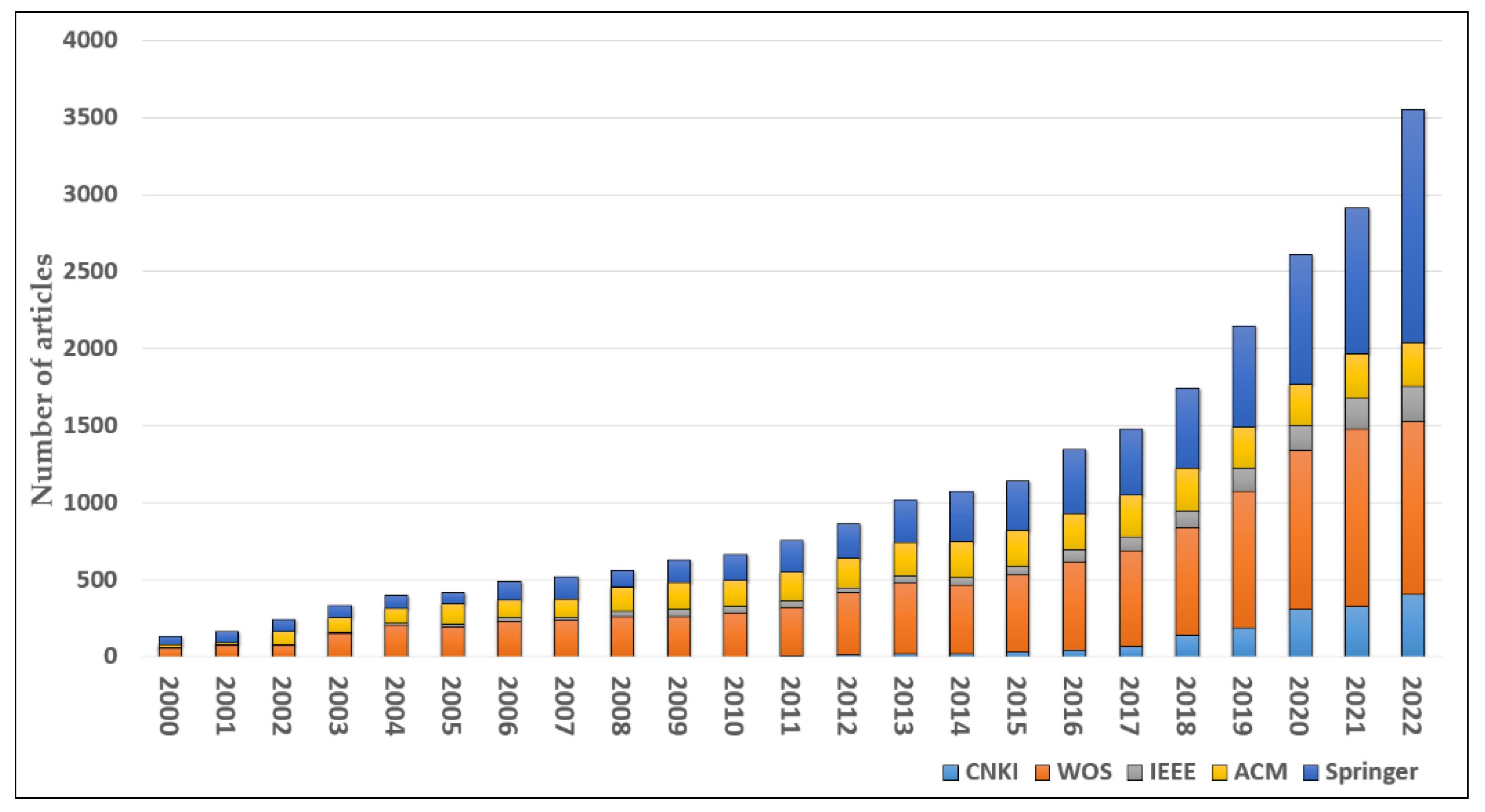
In our investigation of DQ-related research, we used Web of Science (WOS), IEEE Xplore (IEEE), the Association for Computing Machinery (ACM), Springer-Verlag (Springer), and China National Knowledge Internet (CNKI) as the data sources. On one hand, WOS, IEE, ACM, and Springer are four mainstream academic databases used worldwide, where most valuable research papers written in English are collected. On the other hand, CNKI is a widely used academic database in China, where the most valuable research papers written in Chinese are archived. Considering that our research datasets were collected from a major Chinese city, we also chose CNKI as a data source. In the search procedure, we employed the search terms “data quality” and “data cleaning”, and specified the time range of 2000–2022 to retrieve literature from each database (retrieval date: 7 April 2023). After filtering literature that was clearly inconsistent with our research topic, a total of 26,160 papers were obtained as the original papers for this study.

Figure 1 shows the distribution of the related literature from 2000 to 2022. We can clearly see that research on the topic of data quality has experienced explosive growth in recent years. It can be seen that there were relatively few academic studies on data quality in the 2000s, with a total of 134 published papers. A total of 756 papers was published in 2011, while a total of 3552 papers was published in 2022. This indicates that data quality has attracted extensive attention from both domestic and international scholars.

For example, in ref. [7], the authors propose an intelligent preprocessing method for textual data that cleans data containing missing values, grammatical errors, and spelling mistakes. Similarly, ref. [8] explores the impact of noise issues such as misspellings and missing data on the task of detecting different records that refer to the same entity. In the smart grid domain, ref. [9] explores related applications and classifies dirty data into three categories: duplicate data, anomalous data, and incomplete data. Ref. [10] investigates DQ issues such as outliers, incomplete data, duplicate data, and conflicts and develops a tool called Cleanix, which is a prototype system used to clean up these issues. In addition, ref. [1] summarizes data-cleaning techniques and defines four types of DQ problems: missing data, redundant data, data conflicts, and erroneous data. Ref. [11] describes DQ issues such as inconsistency, noise, incomplete, or duplicate values in real-world data.

DQ problems in the public bus transportation system have also been addressed. For example, ref. [12] divided the scope of research on intelligent traffic prediction into four parts: spatiotemporal data, pre-processing, traffic prediction, and traffic applications, where problems such as data anomalies and missing data were analyzed in the data pre-processing stage. Ref. [13] examined issues with data sparsity in bus data, including inconsistencies between operators, GPS location errors, and sporadic GPS sampling. In a similar vein, ref. [14] categorized bus anomalous data into four groups based on the characteristics of bus big data: redundant data, range anomalous data, abnormal data, and missing data. Finally, ref. [15] analyzed four types of DQ problems, namely noisy data, missing values, inconsistency, and redundant data, in taxi track data.

3. Data Quality Taxonomy

In our investigation of DQ-related research, we identified two issues among the existing DQ categories. The first issue is that the same specific data quality problem is assigned two or even several different names. The second issue is that the same specific data quality problem is classified into different categories. We aim to address these two minor issues within our proposed strategies.

Based on 26,160 papers obtained from five databases, we performed a comprehensive statistical analysis of the types of DQ problems found in the literature and classified them into six categories: redundant data, missing data, noisy data, erroneous data, conflicting data, and sparse data. These six categories encompass a range of DQ problems that may be present in a dataset and serve as crucial guides for subsequent data quality improvements for downstream applications.

Table 1. Summarizing and defining data quality issues.

No.	Dirty Data Category	Definition	Statistics on Dirty Data Types in Literature	Literature
1	Redundant data	Data in which the same content appears repeatedly, or there are similar duplicate records.	Duplicate data; duplicate records; duplicate values; duplicate data instances; duplicate data attributes; similar duplicate records	[1,9,10,11,14,15,16,17,18,19,20]
2	Missing data	Missing data in database tables; incomplete data collected.	Incomplete data; missing data; missing values; null values	[1,7,8,9,10,11,12,14,15,21,22,23,24,25,26,27,28]
3	Noisy data	Attribute domain error; refers to data with large deviation.	Incorrect data; anomalous data; range anomalies; inaccurate data; illogical data; invalid data (data taking default values); irrelevant data; noisy data; outliers	[9,10,11,12,13,14,15,23]
4	Erroneous data	Format-related errors, including misspelled attribute values.	Incorrect data; incorrect attributes; incorrect input; spelling errors; incorrect words; incorrect units; incorrect date format	[1,7,8,17,29]
5	Conflicting data	Inconsistent field identification in stored data fields, syntactically or semantically heterogeneous data.	Data inconsistencies; conflicting data; conflicting information; structural errors; conflicting data structures from multiple sources; conflicting naming of data from multiple sources; value-field mismatch; single field holding multiple types of values	[1,10,11,13,15,16,17,30,31,32]
6	Sparse data	The data collected are not evenly distributed in the temporal or spatial dimension, making the data appear discontinuous and incomplete.	Uneven data distribution; discontinuous data; sparse trajectories	[13,33,34,35,36]

provides specific definitions for each category of data quality issues, along with the types of DQ problems identified in the literature and their corresponding references. This classification offers a framework for a thorough and detailed understanding of data quality issues, thereby enabling us to address them more effectively. All the data quality issues mentioned in the cited papers and their studies can be found in Table 1, and all of them can be mapped to the categories we have defined.

In fact, several pieces of literature have already proposed different categorization strategies for DQ problems. We identified two primary challenges during our investigation process. The aforementioned issues are common in current solutions. Firstly, we observed that the same specific data quality issue was assigned different names in different papers in the literature. For instance, as shown in the fourth category in Table 1, some studies describe data errors as “incorrect data”, others as “incorrect attributes”, and yet others use terms like “incorrect input”, “spelling errors”, “incorrect words”, “incorrect units”, “incorrect date format”, etc. These all describe formatting-type errors, but there is no uniform terminology.

Secondly, we also found that the same specific data quality issue was classified into different categories in different studies. For example, some scholars define data anomalies as a type of data error, i.e., data errors contain attribute domain errors and formatting errors. However, most of the papers discuss range anomalies and noisy data separately. Therefore, we further defined attribute domain-related noisy data as data anomalies and format-related dirty data as data errors. Additionally, we noted that there is a significant amount of literature that analyzes inconsistent data in detail. Given that the essence of it is that the stored data are inconsistent with the field identifiers, we categorized this type of dirty data as data conflicts.

In summary, we investigated the data quality issues already present in the literature and reclassified them into new categories. This will facilitate classifying data quality issues into appropriate categories and will be more conducive to subsequent data-cleansing efforts.

4. Data-Cleaning Methods

This study focuses on DQ problems in a real-world big data platform for a city public bus transportation system in China. The corresponding dataset was collected from July 2021 to February 2022. The size of the dataset is 364.6 GB, and the record number of the dataset is 544.48 million. Details about this dataset are listed in

Table 2. Data table information for a domestic city bus dataset.

No.	Table Name	# of Attributes	Description
1	QR_code	15	QR code table
2	Swipe	15	Swipe card table
3	IAO_station	15	Inbound and outbound information table
4	Bluetooth	38	Bluetooth table
5	GPS	13	GPS table
6	Wi-Fi	38	Wi-Fi table
7	Bus_first	28	Vehicle Table 1
8	Bus_second	9	Vehicle Table 2
9	Route	12	Route table
10	Station	12	Station table
11	Route_station	17	Route station table
12	Install_register	25	Vehicle registration table

, in which the second column is the table name, the third column is the number of attributes, and the fourth is the description for each data table. In this paper, we will systematically discuss the DQ problems related to the aforementioned six DQ categories. Firstly, we introduce redundant data, conflicting and erroneous data, and the corresponding data-cleaning methods. Secondly, we describe noisy data in GPS trajectories and propose a solution for noise filtering. Thirdly, we illuminate missing values in the spatiotemporal information of bus arrivals and departures and propose a solution to repair these missing values. We then introduce the pipeline and workflow of noise filtering and map matching in Spark.

4.1. Cleaning Methods for Redundant, Conflicting, and Erroneous Data

There are many participants in a distributed data collection system. These include the terminal, the message middleware, and the backend storage system. Redundant data are caused by network instability and limitations of the data transmission protocol among different participants. For example, a terminal may submit a record to the backend multiple times as the connection is lost and the storage system does not have the ability to detect duplicate data. This ultimately results in the creation of duplicate records within the data-storage system. Several cleaning strategies have been proposed to address this problem. These representative solutions include buffering methods [14], entity recognition methods [16], sorting methods [37], redundant data models/frameworks [38], machine learning [39], and other methods. In this paper, we implement redundant data cleaning on Apache Spark for “QR_code”, “Swipe”, “IAO_station”, “Bluetooth”, “GPS”, and “Wi-Fi” tables.

Conflicting data include DQ issues such as value–field mismatches, a single field containing multiple value types, structural errors, and inconsistent naming of data from multiple data sources. This paper addresses two conflicting data issues: naming conflicts in the “Bus_first”, “Bus_second”, and “Install_register” tables for multi-source data, and inconsistent data in the “Route” and “Install_register” tables, and uses data standardization methods to resolve data conflicts.

Erroneous data include spelling errors in attribute values and other related formatting errors such as misspellings, typos, inconsistent units, inconsistent date formats, and inconsistent value formats. In this paper, we use a customized date conversion function to convert inconsistent date formats in dynamic and static data tables to a standard format, thus completing the cleaning process for erroneous data.

4.2. Cleaning Method for Noisy Data

In GPS trajectory data, anomalous data are referred to as outliers or noisy points. These data usually present scattered, irregular characteristics and are difficult to detect in large volumes of trajectory data. Noise data may place a significant negative impact on trajectory data mining applications. To improve the accuracy of data analysis, these anomalous points in GPS trajectory data need to be cleaned. Generally, GPS anomalous points can be classified into the following two categories:

(1)

Range anomalies: The longitude or latitude of a GPS point outside the specified range, i.e., longitude range between 0 and 180° and latitude range between 0 and 90°. Note that these GPS points outside this area are also considered as anomalous outliers.

(2)

Jump anomalies: Both the longitude and latitude of a GPS point are within the normal range, but there is an extreme distance between a given point and its consecutive points. It means that the GPS point deviates significantly from the original trajectory, resulting in “Jump points” in the trajectory.

To solve the above problem, this paper proposes a solution, which combines the heuristic-based GPS anomaly filtering and Fast Map Matching (FMM) [40] framework for correcting anomalous points in GPS trajectories. Key steps are as follows: Firstly, it applies a heuristic-based GPS anomaly filtering algorithm to the raw GPS trajectory dataset to remove all range anomalies and the obvious jump anomalies. Then, it takes the filtered dataset as input for the FMM algorithm, which incorporates Hidden Markov Models and pre-computation, to correct jump anomalies. This solution not only effectively removes the noises from the raw GPS trajectory dataset but also further improves GPS positioning accuracy.

In the first step, Algorithm 1 is performed to conduct heuristic GPS anomaly filtering. The core idea of this algorithm is to calculate the distance and time difference between two adjacent points, to calculate the instantaneous speed of a bus, and to determine whether it is an anomalous point by a pre-defined speed threshold. During the detection process, we keep and store these weights of the anomalous points. Finally, the anomalies with high weight values are removed from the raw GPS trajectory dataset and the filtered GPS dataset is returned.

Algorithm 1. Heuristic-based GPS anomaly filtering algorithm.
Input: An original GPS trajectory: rawTR,/* each point is a tuple like (numberPlate, timestamp, longitude, latitude)*/Instantaneous speed threshold: threshold. Output: The result after removal of abnormal data: filteredTR.
1	Initialize an empty list: filteredTR
2	for i = 0; i < rawTR.len; i + + do
3	distance = calculateDistance(rawTR [i], rawTR [i + 1])
4	/* calculateDistance() to calculate the distance between two GPS points */
5	time = rawTR [i + 1].timestamp–rawTR [i].timestamp
6	speed = distance/time /* For calculating instantaneous speed */
7	if speed < threshold then
8	rawTR [i + 1].set_weight(rawTR [i + 1].get_weight() + 1)
9	/* If the instantaneous speed is greater than the threshold, add 1 to its weight */
10	rawTR [i + 1].set_is_outlier(true)
11	Else
12	filteredTR.append(rawTR [i])
13	end if
14	end for
15	filteredTR.append(rawTR[last])
16	return filteredTR

In the second step, the FMM (as Algorithm 2 described) matches each trajectory of the filtered GPS dataset to the road network. The FMM algorithm takes a GPS trajectory and the road network as inputs, and outputs a matched GPS trajectory. In detail, it consists of two stages: precomputation and map matching. In the initial stage, the framework precomputes all pairs of shortest paths in the road network below a certain threshold and substitutes these repetitive queries in map matching using a hash table. This hash table is called an Upper Bound Origin Destination Table (UBODT). In the second stage, the framework integrates the Hidden Markov Model (HMM) with precomputation to deduce vehicle paths, taking into account GPS positioning errors and topological constraints. This stage consists of four sub-steps: candidate search (CS), optimal path inference (OPI), complete path construction (CPC), and geometric construction (GC).

Algorithm 2. The fast map matching algorithm.
Input: The original GPS trajectory: rawTR; The road network: network < V, E >; An upper bound origin destination table: ubodt. Output: A matched path: matchedPath.
1	HashMap < point,segment> psegKV = null/* save point and candidate segment */
2	RTree rtree = buildRTree(network)
3	for i = 0; i < rawTR.len; i + + do
4	Point = rawTR[i]
5	proPoint = getProjectPoint(Point,rtree)
6	canSegments = getCandidateSegments(proPoint,rtree)
7	psegKV.put(proPoint,canSegments)
8	end for
9	transitGraph = constructTransitGraph(rawTR,psegKV,rtree)
10	optimalPath = pathInference(transitGraph,ubodt)
11	return optimalPath

The CS step searches the corresponding candidate edges for each point in the trajectory. Based on the HMM model, the OPI step firstly constructs a transition graph of candidate trajectories, and queries the SP (shortest path pair) distance among candidate trajectories. Then, it derives the optimal path of the trajectory. In the CPC step, the SPs of continuous candidate paths in the optimal path will be connected to construct a complete path. The GC step constructs corresponding geometry. Finally, after the above processes, the original GPS trajectory can be corrected onto the road network of the digital map.

In this paper, the accuracy rate is used as a metric to evaluate the algorithm. It is the ratio of the number of successfully matched GPS points to the total number of GPS points. For a given matched GPS point, it must satisfy the following conditions: (a) The GPS point should be located on the road network or very close to the road section; (b) The matched road segments are attached to an actual driving route; (c) The matching error is less than a predefined threshold.

4.3. Cleaning Method for Missing Data

In this section, we introduce missing values in the spatiotemporal information of bus arrivals and departures and then propose a corresponding solution. In this city, each bus has been equipped with a GPS device, which continuously reports its position information to the backend via the mobile internet. When a bus is entering a station, the driver manually reports a message by pressing a button attached to the GPS device. Ideally, it will produce a full ordered sequence for each bus trip, and each element in this sequence contains information about when a bus enters a station and where the station is located, and other information such as “numberPlate”, “routeCode”, and “stopCode”. However, on occasion, some drivers may forget to press the button when the bus arrives at a station, leading to data gaps in the corresponding table.

We propose a solution based on multi-source data fusion to repair the missing data to complete the information on bus arrival and departure. The detailed steps are as follows. Firstly, we check the continuity of “stopCode” by the “Route_station” table to determine whether there are missing data on the information of entering a station. Secondly, missing spatiotemporal information is filled with information “stopCode”, “routeCode”, and “direction”, and then filled with “stationName”, “longitude”, and “latitude” according to information from the “Route_station” table. Finally, we repair the entry “timestamp” in conjunction with each bus’s corresponding GPS trajectory.

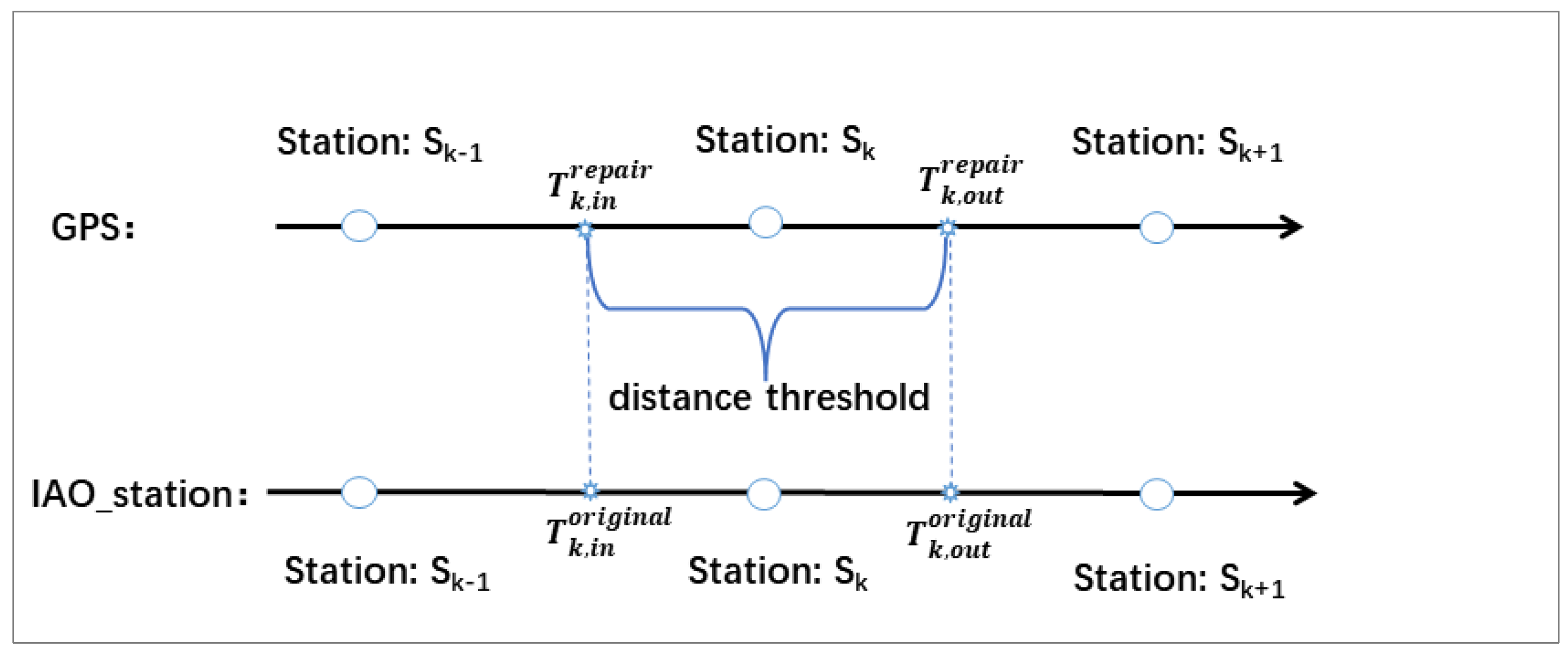
In this dataset, the “GPS” table includes eight fields: “numberPlate”, “timestamp”, “longitude”, “latitude”, “runningStatus”, “vehicleCode”, “speed”, and “direction”, respectively. In the previous steps, we have already successfully repaired the information about “longitude” and “latitude”. In this step, we will find the timestamp ${\mathrm{T}}_{\mathrm{k},\mathrm{in}}^{\mathrm{repair}}$, at which the bus enters the station ${\mathrm{S}}_{\mathrm{k}}$ and the time ${\mathrm{T}}_{\mathrm{k},\mathrm{out}}^{\mathrm{repair}}$, at which the bus leaves the station ${\mathrm{S}}_{\mathrm{k}}$. The method is to measure two different spatiotemporal points: one is the location of a station denoted by a GPS point, and the other is a location listed in the “IAO_station” table. If the distance between these two points is less than the threshold dt, then we can fill the temporal information about the bus’s arrival and departure. The implementation principle is shown in Figure 2:

We choose two metrics from ref. [39] to evaluate our algorithm.

(1)

The Missing Repair Rate (MRR) is a metric to measure the repairing accuracy of the spatial information, which includes ”routeCode”, “stopCode”, “direction”, “station Name”, “longitude”, and “latitude”. MRR is defined by Formulas (1) and (2):

$$\mathrm{MRR}=\frac{1}{N} {{\displaystyle \sum }}_{k=1}^N\delta \left(x_{k,original ,}{x}_{k,repair}\right)\times 100\%$$

(1)

$$\delta \left(x_{k,original ,}{x}_{k,repair}\right)=\left\{\begin{array}{c}1, x_{k,original=}{x}_{k,repair}\\ 0, x_{k,original \ne }{x}_{k,repair}\end{array}\right.$$

(2)

In Formulas (1) and (2), $x_{k,original}$ represents the true value of the missing information of station $S_k$ and $x_{k,repair}$ is the corresponding repaired value. Note that the value in this context is a set of aforementioned fields about spatial information. $\delta \left(x_{k,original},x_{k,repair}\right)$ is a Boolean function that is used to compare two different variables. If two variables are equal, the function returns 1; otherwise, the function returns 0. We take each combination of the original and repair values as a sample. N is the number of samples. The steps of calculating MRR are as follows. Firstly, the algorithm applies the Boolean function to each sample and collects the return value. Secondly, it sums all the returned values. Finally, it calculates the average by the sum and the number of samples.

(2)

The Average Relative Error (ARE) is a metric to measure the repairing accuracy of time dimension. The value of this metric is between 0 and 1. The smaller the value, the closer the repaired value is to the actual value. For example, a value of 0 means the repaired timestamp is equal to the original timestamp. ARE is given in Formula (3):

$$\mathrm{ARE}=\frac{{{\displaystyle \sum }}_{k=1}^N\left| T_k^{repair}-T_k^{original}\right|}{{{\displaystyle \sum }}_{k=1}^N{T}_k^{original}}$$

(3)

where $T_k^{original}$ is the actual arrival or departure timestamp at station $S_k$, and $T_k^{repair}$ is the corresponding repaired timestamp of the missing data. Note that the time is converted to seconds relative to a reference time of “00:00:00”.

(3)

The correlation coefficient (R) is a metric to measure the relationship between a sequence of the repaired values and a sequence of the original values. The value of R is between 0 and 1, and the repairing accuracy is not affected by the number of missing stations if R is equal to 1. R is defined by Formulas (4)–(6):

$$\mathrm{R}=\frac{{{\displaystyle \sum }}_{k=1}^N \left( T_k^{repair}-\overline{T^{repair}}\right)\left(T_k^{original}-\overline{T^{original}}\right)}{\sqrt{{{\displaystyle \sum }}_{k=1}^N{\left( T_k^{repair}-\overline{T^{repair}}\right)}^2} \sqrt{{{\displaystyle \sum }}_{k=1}^N{\left( T_k^{original}-\overline{T^{original}}\right)}^2}}$$

(4)

$$\overline{T^{repair}}=\frac{1}{N} {\displaystyle \sum }_{k=1}^N{T}_k^{repair}$$

(5)

$$\overline{T^{original}}=\frac{1}{N} {\displaystyle \sum }_{k=1}^N{T}_k^{original}$$

(6)

Similarly, where $T_k^{original}$ is the actual arrival or departure timestamp at station $S_k$, and $T_k^{repair}$ is the timestamp that was repaired for the missing data of station $S_k$.

4.4. Parallel Implementation Based on RDD

Figure 3 depicts workflow of noise filtering and map matching for a large-scale GPS trajectory dataset. The input dataset is GPS positioning records stored in HDFS. A dotted box stands for an RDD, and a gray square represents a partition. An arrow denotes the dependency among different RDDs. All of these RDDs form a pipeline to implement noise filtering and map matching for the GPS trajectory dataset. The left side lists the operators being applied to different RDDs, and the right side shows the corresponding RDDs and data structures within them. At each stage in this pipeline, it takes an RDD as input and generates a new RDD by applying an operator to the input RDD. The primary steps are as follows:

Step 1: GPS records input. It loads the GPS record dataset from HDFS into memory and initializes the first RDD. Each element within the RDD represents a GPS record with a set of associated fields.

Step 2: Data extraction. It extracts a set of fields from the original GPS record, including vehicle identity, timestamp, latitude, and longitude. Each element represents a single GPS point.

Step 3: Trajectory generation. It employs the GroupBy operator on the RDD generated in Step 2. Specifically, this operator groups and aggregates trajectory points based on their vehicle identities; it then sorts all points within each group by time and generates a complete trajectory for each vehicle.

Step 4: Data partition. It utilizes the rePartition operator and a User-Defined Function UDF) partitioner on the RDD generated in Step 3, resulting in a new RDD with a varying number of partitions. This data partitioning aims to alleviate data skew among different partitions and enhance the parallelized tasks in subsequent stages. In the newly generated RDD, each element represents a trajectory segment rather than a complete trajectory.

Step 5: Noise filtering. It employs the MapValues and a UDF operator on the RDD generated in Step 4. This UDF implemented a heuristic noise-filtering method (Algorithm 1) to generate filtered trajectory segments.

Step 6: Map matching. It employs the MapValues and a UDF operator on the RDD generated in Step 5. This UDF implements the FMM algorithm (Algorithm 2) to conduct map matching, in which it takes a filtered trajectory segment as input and outputs a matched trajectory segment.

Step 7: Trajectory rebuild. It employs the GroupBy operator on the RDD generated in Step 6. Specifically, this operator groups and aggregates the trajectory segments based on their vehicle identities, sorts all segments by time, merges these sorted segments, and ultimately generates a complete matched trajectory for each vehicle.

Step 8: Matched trajectory output. It saves the RDD generated in Step 7 to HDFS.

Note that it is worth to further discuss the data partitioning technique used in Step 4. The re-partitioning process consists of the following steps: Firstly, the algorithm divides the geographical space into a set of uniform grids. Subsequently, it carries out a spatial intersection between each trajectory in the original RDD and the aforementioned uniform grids. During this process, a complete trajectory might be divided into distinct trajectory segments, with each segment being assigned a unique grid identity. Thirdly, it organizes all segments into separate partitions based on their grid identities, resulting in the creation of the second RDD. Within this RDD, every partition contains all trajectory segments assigned to the same grid.

5. Experimental Setup

5.1. Experimental Environment

All experiments in this paper were performed on an 8-node Spark cluster, with each node equipped with the same hardware and software. The specific hardware configuration information is: 16-core Intel (R) Xeon (R) Silver 4110 CPU @ 2.10 GHz CPU, the memory is 16 GB, the hard disk is 2 TB, and CentOS 7.6 is the node operating system. The software configurations used in the experiments are Hadoop-3.2.0, Spark-3.2.0, Scala-2.12.12, JDK 1.8.0_181, and SBT-1.2.7.

5.2. Experimental Data

This study uses a real-world traffic dataset from a public bus transportation system in a Chinese city. The dataset was collected from July 2021 to February 2022. The dataset is 344.4 GB in size and contains a total of 544.48 million records. It contains 12 different tables covering route stops, vehicle scheduling, and GPS-related information for the bus transportation system. In addition, the specific table information is as follows: The “QR_code” table is 0.3 GB in size and contains 622,900 records; the “Swipe” table is 1.3 GB in size and contains 3,197,700 records; the “IAO_station” table is 4.1 GB in size and contains 10.62 million records; the “Bluetooth” table is 53.9 GB in size and contains 77.84 million records; the “GPS” table is 70.7 GB in size and contains 187.99 million records; and the “Wi-Fi” table is 214.1 GB in size and contains 264.0452 million records. In addition, the basic-static table is 19.82 MB in size and contains 157,100 records.

6. Experimental Results and Analysis

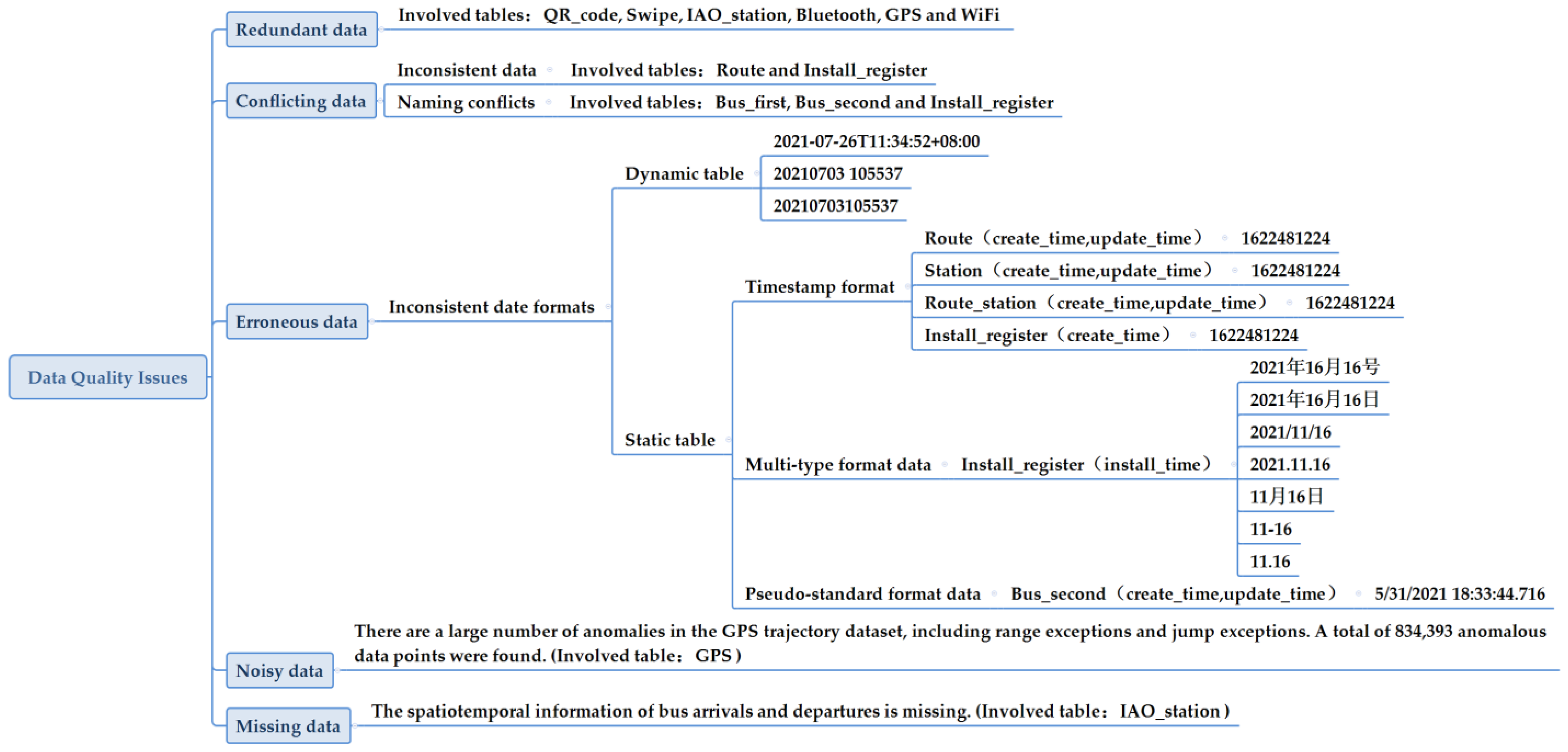
In this section, we first provide an overview of data quality issues across 12 different tables gathered within a real-world urban traffic big data platform. We secondly introduce our methods for cleaning redundant, conflicting, and erroneous data. Finally, we present solutions for filtering GPS noisy data and cleaning missing data. All methods are implemented in Spark, a large-scale data-processing engine, to handle datasets comprising hundreds of gigabytes.

Figure 4 illustrates an overview of data quality issues across 12 different tables collected from a real-world urban traffic big data platform. This figure enumerates data quality issues, identifies the associated tables, and presents representative examples of data quality problems. The data quality issues encompass redundant data, conflicting data, erroneous data, noisy data, and missing data. As an example, we will use the “Install_register” table and the “install_time” field to illustrate a data quality issue. “install_time” is a timestamp that records information about when the operator deployed the data collection terminal on a bus. As we can clearly see from this figure, there are seven different time formats for the same value. On 16 November 2021, a group of construction workers installed numerous data collectors on various public buses. When entering data records into the database tables, seven different time formats were used. Specifically, three of them did not include information about the year. Various characters were used to separate the year, month, and day in the data. We can conclude that a flaw existed in the table design, as it lacked input content format checks, enabling unrestricted user data input.

6.1. Results of Cleaning Redundant, Conflicting, and Erroneous Data

6.1.1. Results of Cleaning Redundant Data

According to the statistics, it can be seen that there are some redundant data in the “QR_code”, “Swipe”, “IAO_station”, “Bluetooth”, “GPS”, and “Wi-Fi” tables. Among them, the “Bluetooth” table has the highest redundancy rate. Specifically, the number of redundant records is 2.98 million, which accounts for 3.8% of the total records. The “QR_code” table has the second highest redundancy rate with a value of 2.8%, which contains 20,828 redundant records. The “Swipe” table has the lowest redundancy rate with a value of 0.17%, which contains 5413 duplicate records. We used the method described in Section 2 to clean the redundant data. The method firstly utilizes Spark to load the raw dataset from HDFS into the memory and transforms it as a dataframe(RDD) for subsequent processing. It then calls the distinct() function to remove the redundant records from the dataframe, creating a filtered dataframe. Finally, it saves the filtered dataframe to HDFS.

6.1.2. Results of Cleaning Conflicting Data

In the field of bus transportation systems, the types of conflicting data are twofold: multi-source data naming conflicts and data inconsistency. The first type refers to the fact that a particular attribute is contained in different tables, but each table has a unique attribute name for that attribute. We used the rule-based approach [41] to identify the relevant data conflict issues. For example, the license plate number has three different attribute names in different tables. The corresponding attribute name in “Bus_first” is called “numberPlate”, in “Bus_second” it is represented by “plateNo”, and in the “Install_register” it is represented by “carNum”. Data inconsistency means that the same entity is named differently in different tables. For instance, consider an entity connected to a specific bus line that requires a unique identifier. In the “Route table”, it is marked as “Business Line 2,” while in the “Install_register” table, it is labeled as “Business 2”. Similarly, “Fan 186 Road” in the “Route” table corresponds to “Fan 186 Line” in the “Install_register” table, and so on.

To address the first issue, this paper uses the data standardization method described in Section 2, which takes “numberPlate” as the unique attribute name for the number plate in all related tables. Furthermore, to address the second issue, this paper provides a catalog of distinct representations of identical entities. By cross-referencing the descriptions of these entities across various tables, it aims to standardize the entity identifiers originating from different sources, ensuring uniformity in format and content. Consequently, this approach safeguards data consistency and facilitates the creation of a conflict-free dataset.

6.1.3. Results of Cleaning Erroneous Data

In the scenario of a bus transportation system, erroneous data are mainly reflected in irregular date formats. This problem is common in several different tables. The date format in the dynamic table contains only two types, while the date format in the static table is diversified. Specifically, there are several different date formats in the static data tables, including timestamp format, pseudo-standard format data “MM/dd/yyyy HH:mm:ss.ms”, and multi-type format data such as “yyyy.MM.dd”, “yyyy/MM/dd”, “MM.dd”, and “MM-dd”, and so on.

To solve the date format problem, we implemented a User-Defined Function (UDF) to convert all dates into a standard format of “yyyy-MM-dd HH:mm:ss”. Data standardization can not only reduce errors and complete the cleaning of data errors, but also help to make data management easier and more effective. It is also very important to improve data quality.

6.2. Results of Cleaning Noisy Data

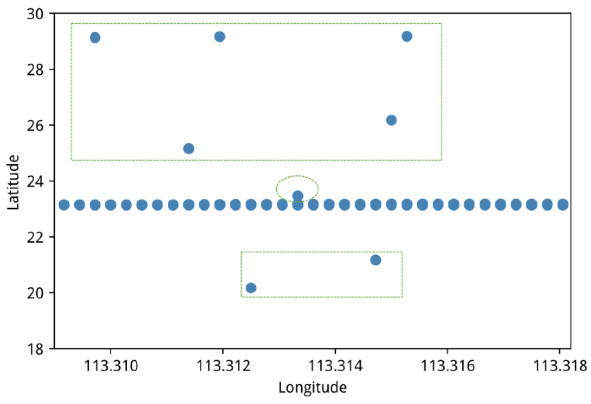
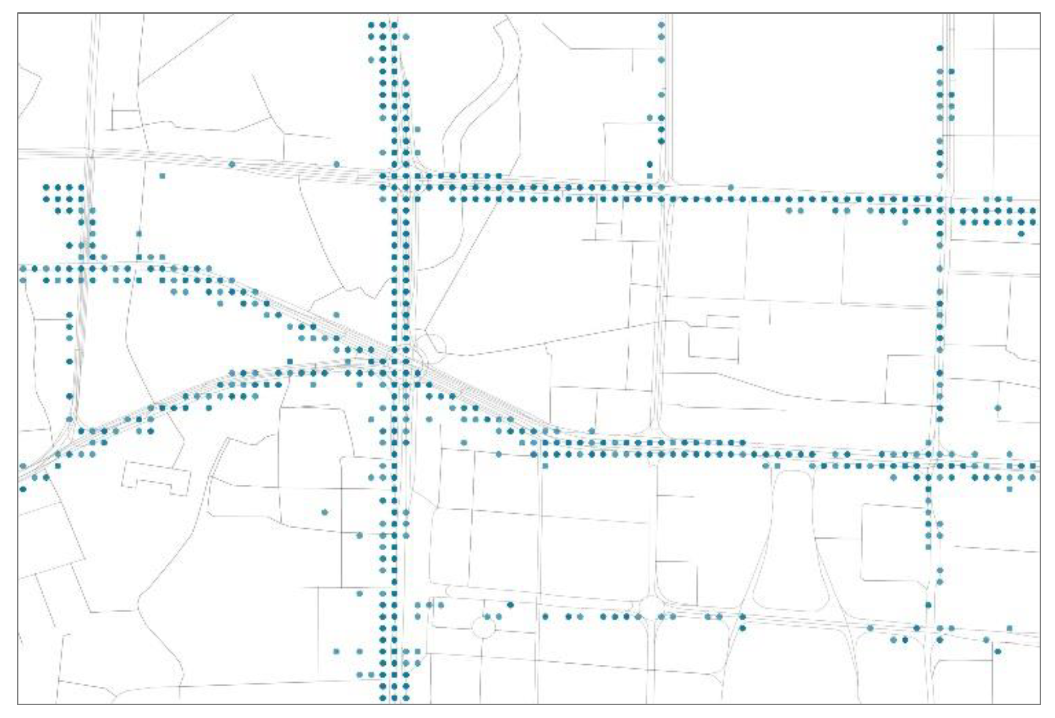
Based on data exploration, we found a large number of anomalies in the GPS trajectory dataset. We selected a trajectory, produced by bus “A000**” on 1 January 2022, to illustrate anomalies and normal GPS points. Note that we replaced part of the true bus number with “**” for privacy reasons. Figure 5 represents a trajectory comprising a sequence of GPS points in order. Upon observing the figure, it becomes evident that numerous range anomalies exist among these points, as exemplified by the rectangular boxes, and there are instances of jump anomalies, illustrated within the oval. This observation signifies the presence of substantial noisy data points within the GPS trajectory dataset. Consequently, the upcoming focus is on designing an effective data-cleaning strategy to eliminate the noise within the GPS trajectory data.

In this subsection, we employ 17.01 million GPS records generated by 132 different buses over the course of one month (January 2022, with 31 days) as input for the data noise-cleaning process. Each record includes a series of fields, such as “numberPlate”, “timestamp”, “longitude”, and “latitude”. Applying Algorithm 1 detected 834,393 abnormal data points, constituting 4.9% of the total data points. Subsequently, we transformed these GPS records into trajectories corresponding to each bus trip, yielding a total of 253,797 GPS trajectories. Additionally, the urban road network data comprises 65,882 nodes and 147,472 directed edges. To compare the effects before and after noise removal, we visualized both the original GPS trajectory and the trajectory after noise removal. Figure 6 shows the original GPS trajectory, revealing that GPS points are scattered around the road, with some not aligning precisely with the road segments.

Figure 7 displays a section of the trajectory after map matching. The left side visualizes trajectory 1, while the right side visualizes trajectory 2. In the figure, the orange circles represent the trajectory before matching, whereas the blue circles represent the trajectory after matching. As depicted, the map matching process has successfully aligned the GPS trajectory.

In this section, we performed noise elimination on the GPS trajectory dataset using a combination of heuristic-based anomaly filtering and the FMM algorithm. The experimental results demonstrate that this filtering algorithm significantly enhances the accuracy of GPS map matching. The combined cleaning method achieves an accuracy rate of 97%, a notable improvement compared to using map matching alone. Figure 8 illustrates the accuracy comparison between our proposed solution and the default solution.

6.3. Results of Cleaning Missing Data

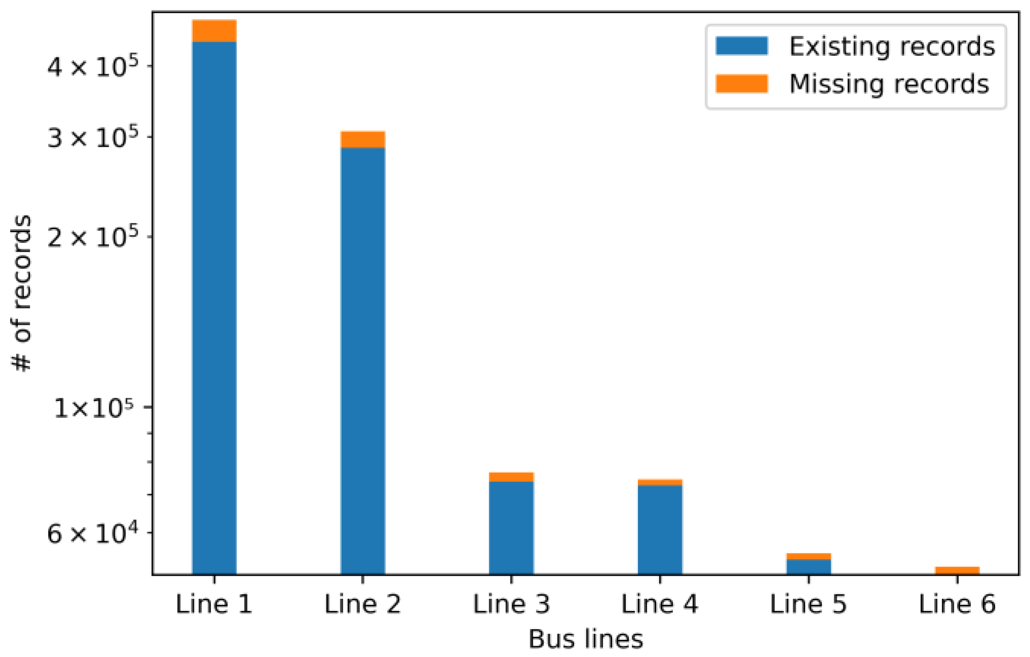
To investigate the distribution of missing data, we employed a data integration operator that connects various tables, including the “IAO_station”, “Bus_first”, and “Route_station” tables. This integration results in the creation of a new table, referred to as “table1,” which encompasses fields such as “numberPlate”, “timestamp”, “routeCode”, “stopCode”, “direction”, “stationName”, “latitude”, and “longitude”. After sorting the records in the temporary table based on the “numberPlate” and “timestamp” fields, we derived “table2”, which contains information about bus arrivals and departures during a given time period. As the “stopCode” on a fixed line is continuous, it can be used as a criterion to determine whether the information on bus arrival and departure is missing. This study shows that there are many gaps in the records on bus arrival and departure stations. As shown in Figure 9, the x-axis represents different bus lines, the y-axis shows the number of records. We found that many records were missing from the records about different bus lines. For instance, Line 1 had 441,986 records in the original data for January 2022. Upon inspecting the “stopCode” field in “Table 2”, we identified a total of 40,756 missing records, equating to a missing rate of 8.44%. This highlights a significant amount of missing data in the “IAO_station” table.

From

Table 3. An example of missing data for bus arrival and departure stations. Note that part of the true bus number was replaced with “**” for privacy reasons.

NumberPlate	Timestamp	RouteCode	StopCode	Direction	StationName	Latitude	Longitude
A001 **	1640993736	08360	08360101	2	Station 1	23.066658	113.294601
A001 **	1640993805	08360	08360101	2	Station 1	23.066658	113.294601
A001 **	1640994539	08360	08360108	2	Station 8	23.075899	113.307739
A001 **	1640994567	08360	08360108	2	Station 8	23.075899	113.307739
A001 **	1640994641	08360	08360109	2	Station 9	23.085596	113.310631

, we can see that there is missing “stopCode” information between 08,360,102 and 08,360,107 for this bus. Considering that bus lines are usually stable, they can be fixed with static line and station information and dynamic GPS trajectory. The specific procedure is as follows: First, it checks the continuity of the “stopCode” through the “Route_station” table to determine whether there are any missing data. Second, for the missing bus arrival and departure information, it fills in information such as “stopCode”, “routeCode”, and “direction”, and then fills in information such as “stationName”, “longitude”, and “latitude” according to the “Route_station” table. At this point, only the “timestamp” information for bus arrival and departure has not been imputed. Finally, combined with the GPS trajectory of the bus, the restoration of the time stamp information of the bus arrival and departure at a station is completed.

In order to validate the missing data imputation solution, we randomly selected a set of samples, each of which has a complete sequence of arrival and departure information for a particular bus trip. We selected one of them to illuminate how we conducted this solution. Table 3 describes this sample, the corresponding license plate number is A001**, the route is 08360, and the time period is from 1 January 2022 07:35:00 to 1 January 2022 08:33:00. The dataset contains complete arrival and departure information for 28 stations, each with two separate records for inbound and outbound. Thus, there are a total of 56 data records. First, the arrival and departure information between (02,07) and (18,23) is randomly removed, and then we apply the aforementioned multi-source data fusion method to impute this sample. The results of three evaluation metrics are shown in

Table 4. Results of cleaning bus arrival and departure time data.

Evaluation Metrics	MRR/%	ARE/%	R
Arrival time	100	0.0690	0.9966
Departure time	100	0.0139	0.9984
Arrival and departure time	100	0.0418	0.9974

, and the details about these repaired values of the arrival and departure timestamps are shown in Figure 7.

From Table 4, it can be seen that for the missing repair ratio of the “routeCode”, “stopCode”, “direction”, “stationName”, “longitude,” and “latitude” repair, the value of MRR achieves 100% and R is also close to 1. The ARE values demonstrate a consistent stabilization below the threshold of 1.0%, which means that most repaired timestamps are very close to the corresponding original values. The above experimental results illustrate that the solution we proposed works well in missing data imputation on bus arrival and departure timestamps. 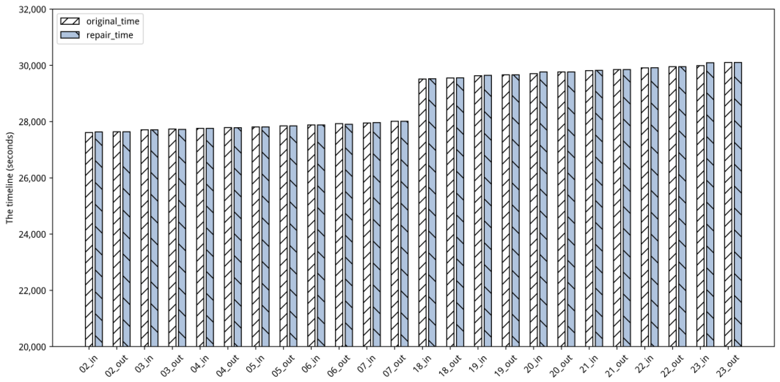Figure 10 also proves this conclusion.

As shown in Figure 10, the x-axis represents a set of different stations belonging to a particular bus route, and the y-axis represents the timeline of the bus trip. The figure shows that the time difference between arrival and departure bus repairs is very small. The sum of time differences in arrivals is 241 s on this trip, and the sum of time differences in departures is 48 s. Among these, 66.67% of the time difference between the original and the repaired timestamps is less than 10 s, 91.67% of the time difference is less than 30 s, and 95.83% of the time difference is less than 60 s. In summary, the effectiveness of the multi-source data fusion cleaning method has been thoroughly demonstrated.

7. Conclusions and Future Work

7.1. Conclusions

In this paper, we began by examining over 20,000 articles related to data quality from five renowned databases. Subsequently, we categorized these studies into six distinct categories based on the specific DQ problems they address. These categories include redundant data, missing data, noisy data, erroneous data, conflicting data, and sparse data. We further delved into the corresponding data-cleaning strategies associated with each category.

Second, we utilized a real-world traffic big data platform and dataset to systematically investigate data quality issues and their corresponding solutions within the realm of public bus transportation systems. Finally, we provided two representative examples: one demonstrating GPS noise filtering and the other addressing missing-value cleaning, both illustrating the effectiveness of our data quality improvement efforts.

The experimental results demonstrate that our GPS noise-filtering solution achieved an accuracy rate of 97%, surpassing the baseline method. Furthermore, our multi-source data fusion approach attained a 100% correct repair rate for bus arrival and departure information in the spatial dimension. The error margin between the repaired timestamps and the actual timestamps was less than 1%, and the correlation coefficient R was also close to 1. These findings provide valuable insights and lessons for enhancing data governance and improving data quality within the public transportation industry.

7.2. Future Work

While this approach provides a validated solution for improving data quality in bus transportation systems, there are still two limitations that need to be addressed: performance and real-time requirements.

On one hand, we have implemented the solution and workflow with multiple stages, but there is room for performance improvement. Data skew exists in these stages due to the default partitioning method. To enhance performance, we plan to implement spatial–temporal partitioning and indexing to efficiently organize datasets in the pipeline. On the other hand, the current solution operates in batch-processing mode, which is insufficient for handling real-time data streaming generated in bus transportation systems. Our next step is to implement our solution using stream-processing engines like Spark Streaming and Flink [41]. This will enable the quick transformation of raw datasets with different data quality problems into high-quality datasets.

By addressing these limitations, we anticipate achieving higher performance and efficiency compared to the current version.