Optical Particle Visualization Technique Using Red–Green–Blue and Core Storage Shed Flow Field Analysis

Abstract

This study uses a flow visualization method to analyze the flow field of a shed-type coal storage shed, comparing and verifying the findings through numerical calculation. Initially, a coal warehouse-scale model is created for flow visualization. Laser-based cross-sectional analysis yields essential flow data, from which red–green–blue values are extracted, and the flow object with the highest G value is selected. Subsequently, as the video frame changes, the moving object is tracked, and the direction is derived. The velocity vector of the moving object within the designated area is derived. Finally, we compare the results of the flow visualization experiment with the simulation outcome. Notably, the error rate in regions characterized by high flow velocity is found to be low, and a high implementation rate is observed in areas with many floating objects to track. Conversely, implementation accuracy is lower in low-velocity fields. Both methods result in a recirculation zone at the top of the inlet, and a flow stagnation region occurs on the upper part of the central wall.

1. Introduction

Coal has plenty of reserves, with several coal types evenly distributed throughout the world. It is a highly economical energy source. However, the rise in the use of fossil fuels has resulted in a global climate crisis. Hence, the world is reducing its dependence on coal. The use of green energy (hydrogen, solar, and nuclear) has increased, reducing greenhouse emissions and air pollution. However, coal-fired power generation is still used in many places. This energy transition will take a long time to be achieved, prompting many countries to strengthen their energy competitiveness considering its relevance to climate change.

A good example is the investment in coal-fired power plants. Many power plants build and operate coal storage sheds to reduce the dust generated when storing coal. Coal stored outdoors generates coal dust because of the wind around it. Constructing an indoor coal storage facility reduces fine dust and provides a stable coal supply. Coal storage sheds (CSS) are classified into shed, dome, and silo types. The most common is the shed-type CSS, which is used in many power plants because it is economical and easy to construct. However, the major challenge with indoor coal storage is the spontaneous combustion of coal [1]. Factors of spontaneous combustion of coal include volatilization characteristics, storage period, size of coal particles, moisture, and impurities [2,3]. Upon exposure to air, coal reacts slowly with oxygen and generates heat [4]. The stages of spontaneous combustion of coal are as follows: the temperature rises in the presence of oxygen, [5,6,7] leading to the initial ignition stage and increasing the temperature of the coal pile. Compounds in coal decompose, producing high amounts of harmful gases. Additionally, oxygen absorption and heat generation in the coal pile increase, and the temperature rises quickly to approximately 84 °C. Coal ignites when it enters the ignition stage, generating a large amount of harmful gas and smoke. Finally, at the late firing stage, the firing spreads [8,9]. The ignition temperature of sub-bituminous coal is approximately 160–170 °C, while the ignition temperature of anthracite is approximately 185 °C. Thermal power plants prefer low-grade coal because it is economical. Low-grade coal has a moisture content of 15% or more and a calorific value of 23,848 kJ/kg, accounting for 47% of global coal reserves, and is cheaper. Therefore, it is the most preferred coal type for thermal power plants. However, low-grade coal causes a decrease in dust collection performance, increases heat loss, and shortens the lifespan of power generation facilities, while its spontaneous combustion remains its most important challenge. The high porosity of low-grade coal, coupled with its moisture content of 30–50%, enables it to react well with oxygen. If spontaneous combustion occurs in the CSS, less carbon monoxide is emitted, posing a significant risk to the safety of field workers [10,11,12]. The safest concentration of carbon monoxide required inside an indoor storage facility is 30 ppm. However, when spontaneous combustion occurs, the concentration of carbon monoxide exceeds 30 ppm. Researchers have studied CSS internal flow characteristics and spontaneous combustion using computational fluid dynamics (CFD). However, large-scale facilities find it challenging to determine CFD values through field experiments. Therefore, the internal flow characteristics of CSS must be analyzed comprehensively.

This study analyzes the internal flow field of CSS using CFD, determines the flow information using laser flow visualization, and presents the methods employed.

2. Introduction of Latest Technologies and Research

Studies are being conducted to minimize the impact of coal power generation systems on the environment. Many laser flow visualization methods have been presented to validate computational fluid dynamics (CFD). Therefore, this section introduces the latest technologies related to research on improving ventilation systems using CFD and experiments involving laser visualization techniques.

Weiwu Ma et al. [13] developed a field-validated model that analyzes the dust dispersion effects of open stockpiles using CFD. Additionally, the closed warehouse structure was comprehensively analyzed and validated for warehouse construction using CFD.

Particle image velocimetry (PIV) values of turbulent flow under unrestrained conditions were determined by Arthur, J. K. [14]. A particle measurement study of turbulent open channel flow was used to examine correlation coefficient characteristics, indicating that the turbulence model function was irrelevant under continuous unrestrained conditions.

An advanced method for a miniaturized PIV system was proposed by Zhuo Fu et al. [15]. He explained the characteristics and performance of this system while evaluating the PIV system and presenting its limitations.

Hanyang Liu et al. [16] designed a milli-reactor using CFD and an artificial neural network and validated the CFD results using the PIV technique. As a result, a safe nuclear reactor design method was proposed. Additionally, he presented an optimal structure that satisfies heat transfer and mixing requirements.

Mičko, P. et al. [17] studied the effect of air pollution on the airflow rate in a clean room. Velocity and particle trajectories were investigated using Ansys Fluent and subsequently validated using the PIV method. As a result, the air changes per hour and airflow velocity accuracy inside the clean room explain the parameters behind the flow characteristics.

Weiliang Tao et al. [18] studied a two-dimensional flow field measurement based on optical flow. The study proposed a new PIV technique that creates a two-dimensional velocity chamber for fluids containing sediment. Compared to existing algorithms, it offers superior smoothness and broad consistency.

A hybrid method that overcomes the limitations of optical flow methods was designed by Liu, T. et al. [19]. This method compensates for changes in illuminance and obtains a refined high-resolution velocity field. A quantitative comparison was made between PIV measurements of circular air jets.

In this literature, many studies have analyzed the flow characteristics using CFD and validated the results using PIV. Therefore, this study examines the internal flow characteristics of thermal power plant CSS using CFD. The simulation results are validated using PIV. The advantages of the flow visualization method proposed in this study are as follows. Extract specified color data and check flow information. Existing PIV and flow visualization experiments are expensive. However, the experiment proposed in this study has an advantage in terms of cost. In addition, it has advantages in analyzing the internal flow fields of large structures and buildings. Flow field analysis results are output relatively quickly.

This thesis is divided into five sections: Section 2 introduces previous research and explains the composition of the thesis; Section 3 describes the methodological approach of numerical calculations and PIV experiments; Section 4 presents and analyzes the findings obtained in the study; and Section 5 presents the conclusions.

3. Methodology

This section describes the research methods for analyzing the internal flow characteristics of coal storage sheds (CSS). This study draws results from two methods. First, the internal flow characteristics of CSS were analyzed using the computational fluid dynamics (CFD) method. Secondly, flow information was extracted using a laser flow visualization method.

3.1. Description of Shad-Type CSS

Thermal power plants generate high-temperature, high-pressure steam through coal combustion. The turbine rotates at high temperatures and high pressure. The thermal power plant is built adjacent to the pier. However, strong winds along the coast scatter coal dust. This challenge results in the pollution of the area around the power plant with coal dust. Although anti-vibration walls are installed around the outdoor coal storage, limitations remain. A photo of the scene of spontaneous combustion of coal in CSS is shown in Figure 1 below. Many power plants are adopting and constructing the shed-type CSS due to its economic advantages, consisting of 16 cells that can store coal. The total volume of CSS is 2,298,367 m³, composed of three floors. The ventilation system of CSS is a natural ventilation system that consists of windows, louvers, and monitor louvers. It has a coal storage capacity of 750,000 tons. The process of storing coal in CSS is as follows: when the coal transfer ship arrives at the port, the coal is unloaded using a conveyor belt; then, the coal is stored in the CSS cell through the telescopic chute; a coal pile shape is formed using a reclaimer at an angle of approximately 40 degrees; and lastly, according to the coal supply schedule, the coal is moved to the boiler building using a conveyor belt.

3.2. Computational Analysis

3.2.1. Control Equation for CFD

In this study, the control equation for analyzing CSS internal flow is as follows. First, a viscous state, incompressible, and turbulent flow field is assumed. Then, a computational analysis is performed, assuming a steady state. The governing equations are the continuity equation, momentum equation, and turbulence transport equation. In order to computationally analyze the governing equations, algebraic equations are discretized. The most widely used k-ε model among turbulence models is shown in Equations (1)–(3) below. In the equation, C₁ and C₂ are empirical constants, and A is the turbulence component.

$$\frac{\partial \left(\rho k\right)}{\partial t}+\frac{\partial }{\partial x_i}\left(\partial u_{i}k\right)=\frac{\partial }{\partial x_i}\left(\mu +\frac{{\mu }_t}{{\sigma }_k}\right)\frac{\partial k}{\partial x_i}+G_k-\rho \epsilon$$

(1)

$$\frac{\partial \left(\rho \epsilon \right)}{\partial t}+\frac{\partial }{\partial x_i}\left(\partial u_i\epsilon \right)=\frac{\partial }{\partial x_i}\left(\mu +\frac{{\mu }_t}{{\sigma }_{\epsilon }}\right)\frac{\partial \epsilon }{\partial x_i}+C_1\frac{\epsilon }{k}{G}_k+C_2\rho \frac{{\epsilon }^2}{k}$$

(2)

$${\mu }_t=\rho C_{\mu }\frac{k^2}{\epsilon }$$

(3)

In general, in a turbulent flow field, changes in physical quantities near the wall are large. Therefore, a dense grid system is needed to improve the accuracy of the analysis. CSS is very large in size and has a complex internal structure. Therefore, in this paper, the wall function is applied to simulate the flow around the wall surface. The CSS grid is a tetrahedron, and the total number of grids is about 8,000,000 cells.

3.2.2. Modeling and Boundary Conditions

This study analyzed the internal flow field of shed-type CSS and determined the results using the flow visualization method. Computational analysis is described below. Ansys Fluent 2021 R2, a CFD S/W is Ansys Fluent 2021 R2, was used to analyze the internal flow field. The modeling photos of CSS and the boundary conditions for computational analysis are shown in Figure 2 and

Table 1. Boundary conditions for computational analysis.

Conditions	Value	Remark
Coal storage	100%	Porous zone Laminar flow zone
Angle of repose	40°
Coal diameter	0.01 m
Porosity	0.2
Inlet velocity	2.0 m/s	1st floor Louver and window
Initial temperature	20 °C
Turbulent model	Standard k-ε model

, respectively. The building is 66 m high and 125 m wide, and the central wall is 28 m high. In the Figure below, The green line indicates the coal pile, the blue arrows show the window inlet and the monitor louver is red. The inclined angle of the coal pile is 40 degrees, assuming a coal pile with 100% coal storage. The diameter of the coal particles is assumed to be 0.01 m, [20] considering the characteristics of the inclined surface of the coal pile. Therefore, the coal pile was set to a porosity of 0.2. The initial boundary condition was set in such a way that air flows in at a speed of 2 m/s from the louvers and windows on the first floor of the CSS. The temperature of the air was 20 °C. The results were output under steady-state conditions, and the turbulence model employed the standard k-ε model commonly used in the industry.

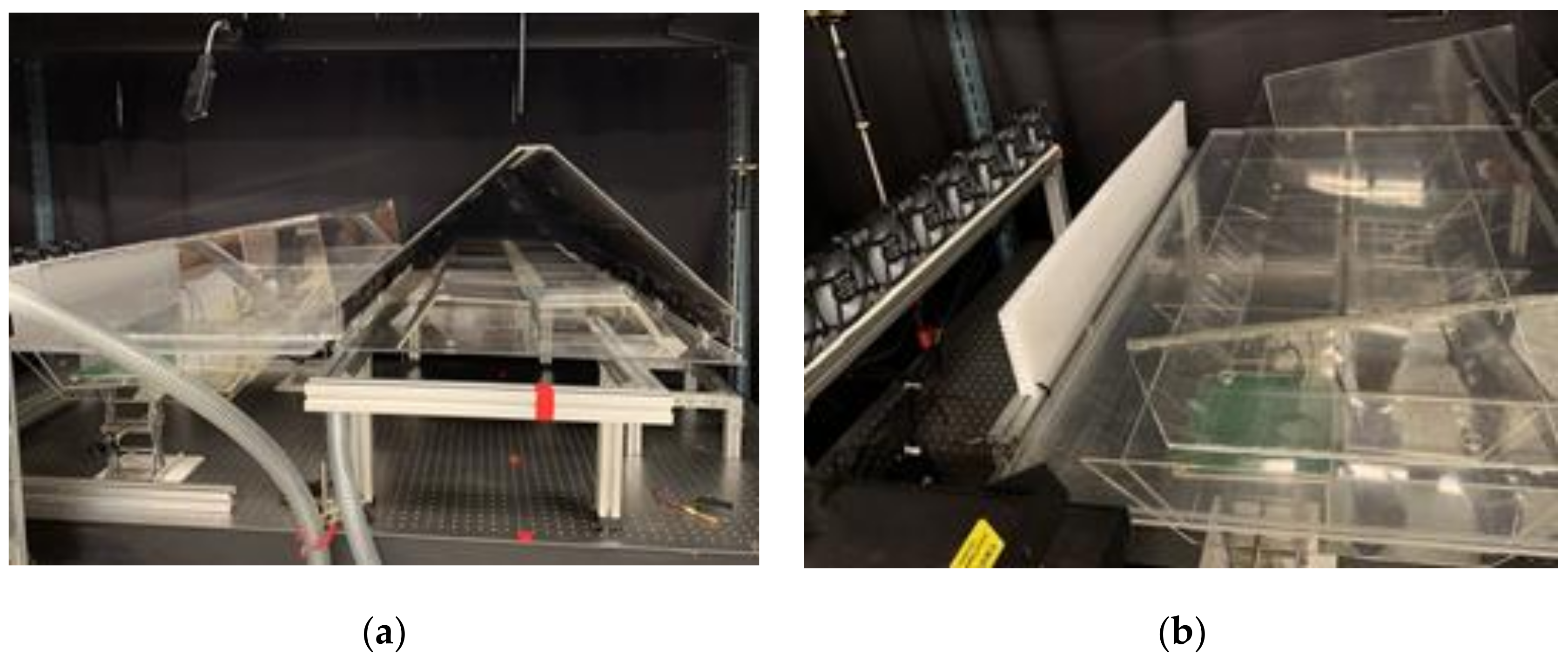
3.3. Verification Experiment Using the Flow Visualization Method

3.3.1. Flow Visualization Experiment Using a Laser

In this study, the CFD flow analysis was determined using flow visualization results. The flow information extraction method that employs the reduced model is explained below. Flow information such as velocity, pressure, and density is extracted in various ways. This study uses a tomography technique to extract flow information from a two-dimensional cross-section formed by a laser light source. The method is as follows: first, an experimental model with a CSS ratio of 1/180 is produced, after which the fan is installed in front of the scale-down model. The wind speed is then realized by adjusting the RGB. The flow information can be seen in the laser cross-section using a smoke-generating device. The data is then obtained by taking a picture of the flow field in the laser cross-section. The configuration diagram and photos of the experimental device are shown in Figure 3 and Figure 4. Blue arrows indicate wind. And the green cross section of the CSS scale model represents the laser extracted flow field.

3.3.2. Laser Source and Wind Device

The light source is an essential factor in cross-sectional photography. A laser is an amplifier of light by stimulated emission and has high energy density and excellent straightness. This experiment uses monochromatic light. Therefore, the difference in refractive index of the laser is not considered. And for tomography experiments, a low-power laser of 500 $\mathrm{m}\mathrm{W}$ is used, and the green wavelength is 0.154. A cylindrical lens is included in the laser to create a two-dimensional plane. Light passing through a cylindrical lens creates flat light with a thickness of 1 mm. Additionally, a video recording device is used to extract real-time information on the flow field. Temporal resolution is dependent on the frame rate. Therefore, video recording devices use image memory and H/W dedicated to video data processing. The FPS of the video device is 29.97. The images were separated by frame, and the image and video were output. The resolution of the image is 2 k, and the size of the image is 2048 $\times$ 1080. Laser tomography is performed in a dark laboratory. In the experimental setup, a flow stabilization device is installed in front of the CSS to stabilize the wind. Through flow stabilization, the turbulent variability of the wind flowing into the CSS window is minimized. Inject seed particles into the fluid. Then, flow information from the cross-section is extracted. The seed particles selected olive oil. The formation of airflow varies depending on the arrangement and complexity of the indoor shape. Therefore, the internal space is simplified, and the Reynolds number is the output. The scale model has a scale of 1/180, and the inflow speed is 6 m/s. The Reynolds number of the experimental model is 99,265. The CAARD model is one of the box-type large building models. The CAARD model is a wind tunnel experiment research model and has been widely used in research. According to the model, the Reynolds number for large buildings is approximately 300,000 or higher. According to M. Valikibi’s study, flows at high Reynolds numbers have statistically similar trends [21]. Since the Reynolds number is over 20,000 in this experiment and CFD simulation, trend analysis is possible.

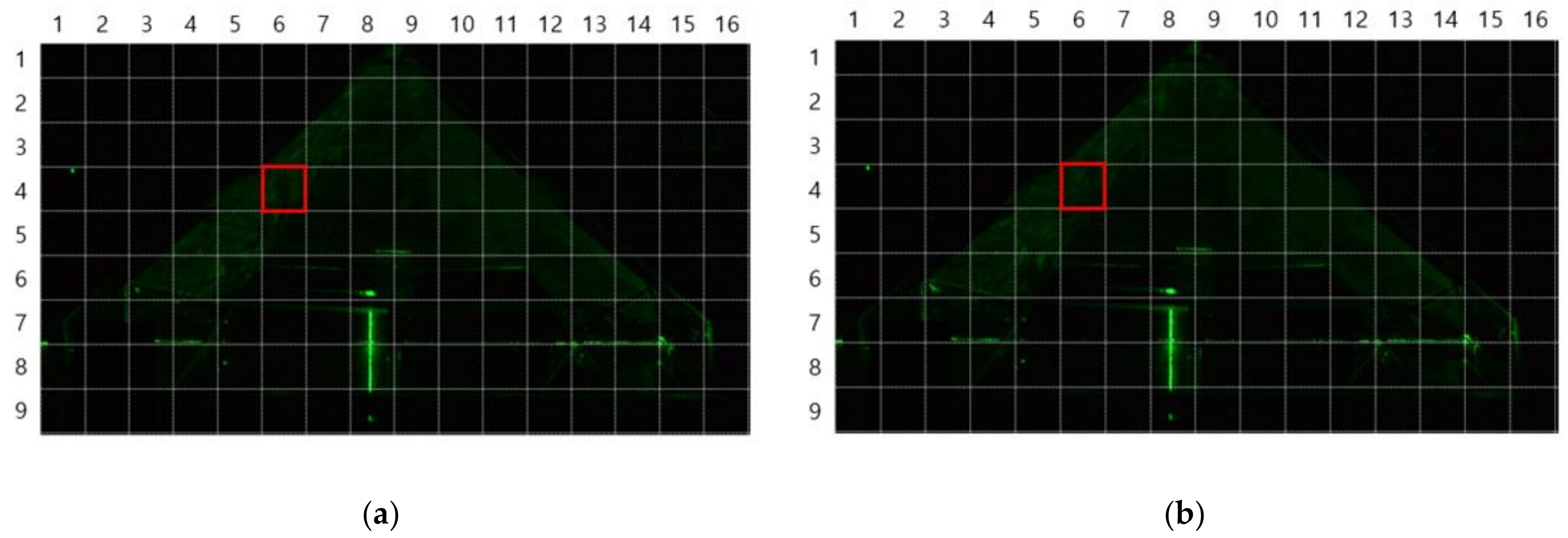
3.3.3. Flow Field Extraction Method

The method for extracting flow information using laser flow visualization is explained. First, the video captured is stored as an image for each frame. Red–green–blue (RGB) values were extracted from the flow information image and stored with RGB representing the three primary colors of light in computer graphics. The RGB color coordinate system is attached in Figure 5. It represents a cube’s R, G, and B values with each cube axis as a color scale expressed in RGB space [22,23]. Each light source has a maximum value of 255. The coordinates of red are defined as (255, 0, 0), green as (0, 255, 0), blue as (0, 0, 255), Magenta as (255, 0, 255), Cyan as (0, 255, 255) and Yellow as (255, 255, 0). The origin of the coordinates (0,0,0) is represented in black, and the coordinates (255,255,255) are represented in white. The line connecting the origin and the white point is grayscale. In this study, flow information was extracted using a green laser to track the R-value. Big and small eddies exist in the visualized flow field, including various turbulence components. The turbulent flow component with volatility is identified as noise and eliminated. Therefore, it is converted into a 9 $\times$ 16 main matrix to normalize the visualization result. The area of each matrix is used for visualization analysis. There are flow objects within the segmented area of the flow field. The top 0.5% of the RGB value is defined as a flow object, and the segmented area tracks the flow object’s progress.

4. Results of Flow Characteristics Analysis

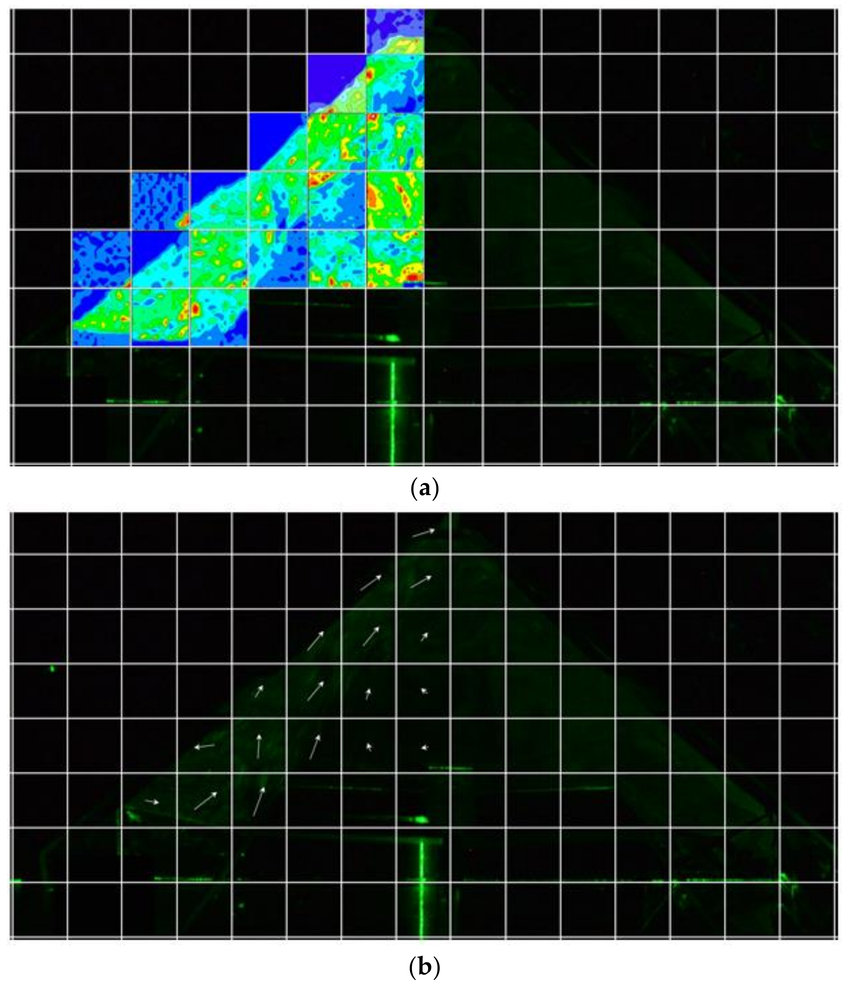
4.1. Experimental Results Using the Flow Visualization Method

The results of the flow information extracted using the laser flow visualization method are described below. This study defines the main area of 9 × 16 size as A(i,j). Figure 6 shows the partition area for extracting flow information. The red square is partition area A(4,5). Then, each main area A(i,j) is divided into sub-areas of 9 × 9 size as a(i,j). Figure 7 shows the divided sub-area. In sub-area a(i,j), RGB values are extracted from nine white dots, as shown in Figure 7. A green laser was used to extract the G-value from RGB data. A total of 729 G-values were extracted from A(4,6) and 26,244 G-values were extracted from the flow field to be analyzed.

The G-value from the output image was extracted with the maximum G-value among the extracted G-values, defined as a flow object. Figure 8 shows the distribution of G-values in the partition area A(4,6). A higher G-value means brighter green. About 61% of the G-values are between 7 and 11, with a maximum value of 30. Next, the contrast and background noise of the image were removed, and a flow object was selected. A flow object is a region with the highest G-value. Therefore, in this study, the range of G_peak values was set to the top 0.5%.

Figure 9 shows the flow object at A(4,6) using the G-value. The location of each G_peak is indicated by a red circle. In the first image (a), the flow objects are defined as G_peak,1-1 and G_peak,2-1, while in the second image (b), the flow objects are defined as G_peak,1-2, and G_peak,2-2, respectively. Image (a) shows 2 points where the G-value is included in the top 0.5%, while in image (b), the two flow objects move to the next position, making it necessary to track the movement of two flow objects.

Table 2. Flow object location information and G-value.

Flow Object (Objn-m)	X-Y Coordinates	Gpeak Value	Coordinates Image
Obj1-1	(2.159, −5.305)	30
Obj1-2	(5.359, −2.584)	27
Obj2-1	(3.008, −7.649)	27
Obj2-2	(6.497, −4.899)	26

shows the location of G_peak at A(4,6). The G_peak,1-1 of the first flow object is 30. G_peak,1-2 in the next image is 27. The second flow object has G_peak,2-1 to be 27, and G_peak,2-2 as 26. The maximum value changed is 3 as the flow object moves to the next image. Each G_peak point is the internal point of the flow object. The frame unit changes as the internal point moves. Therefore, the G_peak point can be defined as the movement of the flow object. In this paper, the internal point of the flow object is defined as Obj_n-m.

Figure 10 shows the internal point of the flow object in the X-Y coordinate system. Both vectors are converted into one vector in the specified area. The vector of the first flow object and the vector of the second flow object are shown in Figure 10. Elements of the flow field are extracted by connecting points G_peak,1-1 and G_peak,1-2 and points G_peak,2-1 and G_peak,2-2. Then, an average velocity vector is formed using the two vectors. The conversion of two velocity vectors to an arithmetic average is only possible given the same starting point and constant acceleration. Therefore, this study proposes that the internal points of the two flow objects in the specific area are one internal point. After moving the starting point of the two velocity vectors to the origin, it is converted into an average velocity vector. Figure 11 shows the flow information extracted from A(4,6) through this procedure. In the Figure 11, the two dotted arrows indicate the movement of the two flow objects. And the average vector of the two vectors is shown in blue. Figure 12 shows the result of extracting flow information by applying this method to all divided areas. Figure 12a shows the distribution of G values extracted using the RGB visualization method. Figure shows the distribution of G-value in each partition. Then, the directionality of the G-value is derived using the above average vector conversion method. The results of extracting vector information for the entire flow field are shown in Figure 11b below. Velocity components extracted from the flow field are indicated by white arrows.

4.2. Comparison of Results of Flow Visualization Experiment and Computational Analysis

This section compares and analyzes the results of computational fluid dynamics (CFD) simulation and flow visualization experiments. Analysis of trends is possible given that the Reynolds number is over 20,000 in this experiment and CFD simulation. Figure 13 shows the velocity information of the flow visualization experiment and CFD simulation. In Figure 13c, the red vector is the average velocity vector derived from the flow visualization experiment. Wind from the first-floor windows and louvers of coal storage sheds (CSS) rises through the slope of the coal pile. It is emitted through the upper monitor louver. The comparison results according to the characteristics of each flow field are shown in Figure 14 below. The gray velocity vector is the CFD result. And the red vector is the result of the visualization experiment. Each flow field characteristic is marked in red. As shown in Figure 14a, the implementation rate is relatively high in the partition area from A(6,3) to A(6,1). Given that the flow speed is fast with many flowing objects, that area implements G_peak relatively accurately. As a result, the error rate is low because flow information for tracking is abundant. Next, the results in the recirculation area are shown in (b). Airflow rises through the slope of the coal pile, and rotational flow occurs. In both the simulation results and the visualization experiment results, a recirculation area occurs in A(6,2), A(6,3), and A(6,5), respectively. However, in A(4,3) above the recirculation area, the two results do not align. At point A(4,3), the flow direction changes rapidly, and at this point, the error rate is high. Therefore, it becomes necessary to further divide the area. Both the stagnant and recirculating areas at the top of the central wall are shown in Figure 14c with a relatively low velocity. After carrying out both simulation and visualization experiments, the same recirculation area with low velocity is formed in both areas A(5,6), A(5,5), A(4,5), and A(3,6). However, in area A(4,6), an error occurs between the two results due to the slow flow velocity. Therefore, a thorough summary of the findings proved that the stagnant area existed at the top of the central wall, and the recirculation area also formed identically there.

The error rates of the computational analysis results and flow visualization experiments derived from this study are as follows. In this study, the Reynolds number for analysis and experiment is over 20,000, so trend analysis is possible. Therefore, assuming a flow field of the same size, the size and direction components of the velocity vector are examined. Figure 15 below shows an analysis of the flow field. Direction and magnitude components are output from the velocity of each segment. Below (

Table 3. Analysis of flow characteristics using CFD and flow visualization experiment results.

		CFD Results				Flow Visualization Experiment
		Length of Vector			Direction of Vector	Length of Vector			Direction of Vector
		a	b	c		a	b	c
High velocity area	A(6,3)	0.85	0.83	1.18	45.68	1.22	0.52	1.32	66.91
	A(5,3)	0.77	0.59	0.97	52.54	1.02	0.07	1.02	86.07
	A(5,4)	0.90	0.60	1.08	56.31	1.02	0.48	1.13	64.79
	A(4,4)	0.77	0.46	0.89	59.14	0.77	0.74	1.06	46.14
	A(3,4)	0.51	0.38	0.63	53.31	0.78	0.79	1.11	44.63
	A(3,5)	0.66	0.59	0.88	48.20	0.83	0.79	1.14	46.41
	A(2,5)	0.52	0.66	0.84	38.23	0.66	0.99	1.19	33.69
	A(2,6)	0.61	0.76	0.97	38.75	0.48	1.00	1.11	25.64
	A(1,6)	0.43	0.66	0.78	33.08	0.30	1.09	1.13	15.38
Recirculation Area (inlet)	A(6,1)	0.66	0.83	1.06	218.49	0.06	0.65	0.65	354.73
	A(6,2)	0.83	0.73	1.10	48.67	0.77	1.13	1.36	34.27
	A(5,2)	0.43	0.52	0.67	219.58	0.09	0.96	0.96	185.35
	A(5,3)	0.77	0.59	0.97	52.54	1.02	0.07	1.02	86.07
	A(4,3)	0.10	0.37	0.38	195.12	0.47	0.34	0.58	54.12
Recirculation Area (wall)	A(5,5)	0.00	0.25	0.25	180.00	0.32	0.15	0.35	115.12
	A(5,6)	0.28	0.24	0.36	228.24	0.06	0.29	0.29	191.69
	A(4,5)	0.39	0.27	0.47	55.30	0.44	0.15	0.46	71.17
	A(4,6)	0.39	0.24	0.45	238.39	0.20	0.32	0.37	148.00
	A(3,6)	0.20	0.38	0.43	27.77	0.39	0.33	0.51	49.76

), a refers to the x component of the velocity vector, b refers to the y component, and c refers to the size. The direction is expressed as an angle from the origin. In both results, the error rate in predicting the directional component of the flow field is about 10.45%. Large errors occurred in relatively slow flow fields. Therefore, as mentioned earlier, it is necessary to create a smaller grid in the recirculation area and areas with slow flow velocity.

5. Conclusions

This paper compares the results of computational analysis and flow visualization experiments to analyze the internal flow characteristics of shed-type coal storage sheds (CSS) at thermal power plants. The results obtained are as follows:

In the area where many flow objects exist, the error rate between the computational fluid dynamics numerical calculation result and the flow visualization experiment result is low. Additionally, it is implemented relatively accurately even in areas where high-speed rotational flow occurs, whereas areas with low-velocity fields and few flow objects for tracking recorded a high error rate. Therefore, the boundary of the recirculation zone and the slow velocity field must be subdivided into parts smaller than the surroundings. This makes it necessary to expand the selection range of flow objects to track their flow.

From the computational analysis and flow visualization experiments, all recirculation areas occurred at the same location. A flow stagnation region appeared at the top of the central wall. Therefore, it is highly possible to detect high carbon monoxide concentrations in the stagnant area. It is necessary to consider the application of a local exhaust system around the central wall to improve the ventilation performance of the shed-type CSS.

In this study, the results of the internal flow characteristics of CSS were derived using computational analysis and flow visualization experiments. The disadvantage of PIV experiments is their high cost. Economic experiments are possible using the RGB particle tracking method presented in this study. However, the uncertainty of the experimental results must also be considered. Additional research is needed to improve the uncertainty and precision of the experiment. The results of this paper can be used as primary data for RGB particle tracking and the design of CSS ventilation systems.

References

1. Wang, F.; Ji, Z.; Wang, H.; Chen, Y.; Wang, T.; Tao, R.; Su, C.; Niu, G. Analysis of the Current Status and Hot Technologies of Coal Spontaneous Combustion Warning. Processes 2023, 11, 2480. [Google Scholar] [CrossRef]
2. Küçük, A.; Kadıoğlu, Y.; Gülaboğlu, M.Ş. A study of spontaneous combustion characteristics of a Turkish lignite: Particle size, moisture of coal, humidity of air. Combust. Flame 2003, 133, 255–261. [Google Scholar] [CrossRef]
3. Kadioglu, Y.; Varamaz, M. The effect of moisture content and air-drying on spontaneous combustion characteristics of two Turkish lignites. Fuel 2003, 82, 1685–1693. [Google Scholar] [CrossRef]
4. Li, L.; Ren, T.; Zhong, X.; Wang, J. Study of the Oxidation Characteristics and CO Production Mechanism of Low-Rank Coal Goaf. Energies 2023, 16, 3311. [Google Scholar] [CrossRef]
5. Kelemen, S.R.; Kwiatek, L.M. Physical properties of selected block Argonne Premium bituminous coal related to CO2, CH4, and N2 adsorption. Int. J. Coal Geol. 2009, 77, 2–9. [Google Scholar] [CrossRef]
6. Han, F.S.; Busch, A.; Krooss, B.M.; Liu, Z.Y.; Yang, J.L. CH4 and CO2 sorption isotherms and kinetics for different size fractions of two coals. Fuel 2013, 108, 137–142. [Google Scholar] [CrossRef]
7. Liu, S.M.; Sun, H.T.; Zhang, D.M.; Yang, K.; Wang, D.K.; Li, X.L.; Long, K.; Li, Y.N. Nuclear magnetic resonance study on the influence of liquid nitrogen cold soaking on the pore structure of different coals. Phys. Fluids 2023, 35, 012009. [Google Scholar] [CrossRef]
8. Tang, Y.B.; Wang, H.A. Experimental investigation on microstructure evolution and spontaneous combustion properties of secondary oxidation of lignite. Process Saf. Environ. 2019, 124, 143–150. [Google Scholar] [CrossRef]
9. Querol, X.; Zhuang, X.; Font, O.; Izquierdo, M.; Alastuey, A.; Castro, I.; van Drooge, B.L.; Moreno, T.; Grimalt, J.O.; Elvira, J.; et al. Influence of soil cover on reducing the environmental impact of spontaneous coal combustion in coal waste gobs: A review and new experimental data. Int. J. Coal Geol. 2011, 85, 2–22. [Google Scholar] [CrossRef]
10. Lide, D.R. CRC Handbook of Chemistry and Physics, 88th ed.; CRC Press: Boca Raton, FL, USA, 2007. [Google Scholar]
11. Das, M.; Salinas, V.; LeBoeuf, J.; Khan, R.; Jacquez, Q.; Camacho, A.; Hovingh, M.; Zychowski, K.; Rezaee, M.; Roghanchi, P.; et al. A Toxicological Study of the Respirable Coal Mine Dust: Assessment of Different Dust Sources within the Same Mine. Minerals 2023, 13, 433. [Google Scholar] [CrossRef]
12. National Academies of Sciences, Engineering and Medicine. Monitoring and Sampling Approaches to Assess Underground Coal Mine Dust Exposure; National Academies of Sciences, Engineering and Medicine: Washington, DC, USA, 2018. [Google Scholar]
13. Ma, W.; Du, W.; Guo, J.; Wu, S.; Li, L.; Zeng, Z. Dust Dispersion Characteristics of Open Stockpiles and the Scale of Dust Suppression Shed. Appl. Sci. 2022, 12, 11568. [Google Scholar] [CrossRef]
14. Arthur, J.K. PIV Measurements of Open-Channel Turbulent Flow under Unconstrained Conditions. Fluids 2023, 8, 135. [Google Scholar] [CrossRef]
15. Fu, Z.; Li, K.; Pang, Y.; Ma, L.; Wang, Z.; Jiang, B. Study on Water Jet Characteristics of Square Nozzle Based on CFD and Particle Image Velocimetry. Symmetry 2022, 14, 2392. [Google Scholar] [CrossRef]
16. Liu, H.; Wang, C.; Wang, R.; Yang, X. Design, Heat Transfer, and Visualization of the Milli-Reactor by CFD and ANN. Processes 2022, 10, 2329. [Google Scholar] [CrossRef]
17. Mičko, P.; Hečko, D.; Kapjor, A.; Nosek, R.; Kolková, Z.; Hrabovský, P.; Kantová, N.Č. Impact of the Speed of Airflow in a Cleanroom on the Degree of Air Pollution. Appl. Sci. 2022, 12, 2466. [Google Scholar] [CrossRef]
18. Tao, W.; Liu, Y.; Ma, Z.; Hu, W. Two-Dimensional Flow Field Measurement Method for Sediment-Laden Flow Based on Optical Flow Algorithm. Appl. Sci. 2022, 12, 2720. [Google Scholar] [CrossRef]
19. Liu, T.; Salazar, D.M.; Fagehi, H.; Ghazwani, H.; Montefort, J.; Merati, P. Hybrid Optical-Flow-Cross-Correlation Method for Particle Image Velocimetry. J. Fluids Eng. 2020, 142, 054501. [Google Scholar] [CrossRef]
20. Du, B.; Liang, Y.; Tian, F.; Guo, B. Analytical Prediction of Coal Spontaneous Combustion Tendency: Pore Structure and Air Permeability. Sustainability 2023, 15, 4332. [Google Scholar] [CrossRef]
21. Vallikivi, M.; Hultmark, M.; Smits, A. Turbulent boundary layer statistics at very high Reynolds number. J. Fluid Mech. 2015, 779, 371–389. [Google Scholar] [CrossRef]
22. Kim, G. Optical Design Optimization for LED Chip Bonding and Quantum Dot Based Wide Color Gamut Displays; University of California: Irvine, CA, USA, 2017; Available online: https://www.proquest.com/dissertations-theses/optical-design-optimization-led-chip-bonding/docview/2031612971/se-2 (accessed on 18 June 2022).
23. Masaoka, K.; Nishida, Y.; Sugawara, M.; Nakasu, E. Design of Primaries for a Wide-Gamut Television Colorimetry. IEEE Trans. Broadcast. 2010, 56, 452–457. [Google Scholar] [CrossRef]
Figure 1. Coal-fired power plant shed-type coal storage shed: (a) inside the CSS where spontaneous combustion of coal occurred; (b) coal compression work to prevent the spread of spontaneous combustion of coal.
Applsci 13 10997 g001
Figure 2. Structure and shape modeling of a shad-type coal storage shed.
Applsci 13 10997 g002
Figure 3. Schematic diagram of flow visualization experiment equipment.
Applsci 13 10997 g003
Figure 4. Flow visualization experimental device using the laser tomography method: (a) shaded CSS-scale model and fluid equalizer; (b) wind generator and air tunnel.
Applsci 13 10997 g004
Figure 5. Schematic of the RGB color model.
Applsci 13 10997 g005
Figure 6. Flow information of the laser cross section and position of A(4,6) (red square) through flow visualization experiment: (a) the first image of the flow visualization experiment video; (b) the second image of the flow visualization experiment video.
Applsci 13 10997 g006
Figure 7. Additional partition image and G-value extraction point at A(4,6): (a) the first image of the flow visualization experiment video; (b) the second image of the flow visualization experiment video.
Applsci 13 10997 g007
Figure 8. Distribution bar graph of the G-value in A(4,6).
Applsci 13 10997 g008
Figure 9. Three-dimensional graph describing the location and movement of the Gpeak in A(4,6): (a) Gpeak location information in the first image; (b) Gpeak location information in the second image.
Applsci 13 10997 g009
Figure 10. Velocity vector of a flow object in an X–Y coordinate system.
Applsci 13 10997 g010
Figure 11. The average velocity vector at A(4,6) derived from the velocity vectors of the two flow objects.
Applsci 13 10997 g011
Figure 12. G-value and velocity vector in the partitioned area: (a) G-value information in the internal flow field of shad-type CSS; (b) velocity vector using flow information derived through visualization experiments.
Applsci 13 10997 g012
Figure 13. Comparison of velocity vectors between flow visualization experiments and computational analysis: (a) velocity vector of visualization experiment results; (b) velocity vector of CFD computational analysis results; (c) overlap comparison between visualization test results and computational analysis results.
Applsci 13 10997 g013
Figure 14. Comparison of results according to flow characteristics: (a) area of high-velocity flow rising through the slope of a coal pile; (b) recirculation area adjacent to the inlet; (c) fluid stagnation region at the top of the coal pile.
Applsci 13 10997 g014
Figure 15. Three-dimensional graph describing the location and movement of the Gpeak in A(4,6).
Applsci 13 10997 g015