Article

Prediction and Comparison of In-Vehicle CO2 Concentration Based on ARIMA and LSTM Models

1
School of Architecture and Transportation Engineering, Guilin University of Electronic Technology, Guilin 541004, China
2
Guangxi Research Centre for Intelligent Building and Habitat Engineering, Guilin 541004, China
3
Guangxi Key Laboratory of Intelligent Transportation, Guilin 541004, China
4
Guangxi Police College, Nanning 530022, China
*
Author to whom correspondence should be addressed.
Appl. Sci. 2023, 13(19), 10858; https://doi.org/10.3390/app131910858
Submission received: 6 August 2023 / Revised: 25 September 2023 / Accepted: 27 September 2023 / Published: 29 September 2023
(This article belongs to the Special Issue Environmental Contamination and Human Health)

Abstract

:
An increase in the carbon dioxide (CO2) concentration within a vehicle can lead to a decrease in air quality, resulting in numerous adverse effects on the human body. Therefore, it is very important to know the in-vehicle CO2 concentration level and to accurately predict a concentration change. The purpose of this research is to investigate in-vehicle concentration levels of CO2, comparing the accuracy of an autoregressive integrated moving average (ARIMA) model and a long short-term memory (LSTM) model in predicting the change in CO2 concentration. We conducted a field test to obtain in-vehicle original concentration data of CO2 while driving, establishing a prediction model of CO2 concentration with ARIMA and LSTM. We selected mean absolute percentage error (MAPE) and root mean squared error (RMSE) as the evaluation indicators. The findings indicate the following: (1) With the vehicle windows closed and recirculation ventilation mode activated, in-vehicle CO2 concentration increases rapidly. During testing, CO2 accumulation rates were measured at 1.43 ppm/s for one occupant and 3.52 ppm/s for three occupants within a 20 min driving period. Average concentrations exceeded 1000 ppm, so it is recommended to improve ventilation promptly while driving. (2) The MAPE of ARIMA and LSTM prediction results are 0.46% and 0.56%, respectively. The RMSE results are 19.62 ppm and 22.76 ppm, respectively. The prediction results demonstrate that both models effectively forecast changes in a vehicle’s interior environment CO2, but the prediction accuracy of ARIMA is better than that of LSTM. The research findings provide theoretical guidance to traffic safety managers in selecting suitable models for predicting in-vehicle CO2 concentrations and establish an effective in-vehicle ventilation warning control system.

1. Introduction

Individuals spend a significant amount of time in indoor environments, including automobiles. A survey conducted among Americans revealed that 88% of their day is spent indoors, and 7% is spent in a vehicle [1,2]. Therefore, indoor air quality is closely linked to the health, comfort, well-being, and productivity of occupants [3]. Furthermore, the air pollution levels within a vehicle’s interior environment exceed those of indoor living environments [4]. Therefore, we should pay attention to the air quality issue within the vehicle’s interior environment, and the number of studies in this field is increasing [5]. To ensure thermal comfort while driving, people will close windows and use air conditioning, particularly during winter and summer. In a tropical country like Thailand, air conditioning is utilized throughout almost the entire year due to the hot climate, and people commonly utilize recirculation (RC) ventilation mode because it can reduce fuel consumption [6]. When occupants operate air conditioning based on their personal preferences in a vehicle, they may not be aware of the issues caused by RC ventilation mode and closed windows: the elevated concentration of carbon dioxide (CO2) in a vehicle due to human respiration within a small, enclosed space and a low air ventilation rate. In order to investigate the level of CO2 concentration in vehicles during driving, numerous scholars have conducted field measurements of CO2 concentration in small vehicles. For instance, Tolis et al. [7] observed that after 15 min of driving, the CO2 concentration in a vehicle reached 5000 ppm. Luangpresert et al. [6] observed that the concentration of CO2 increased to 10,000 ppm after 33 min of driving. In a survey of taxi air quality, it was discovered that CO2 levels reached 3000 ppm within 45 min of operation and remained above this threshold for over four hours [8]; Barnes et al. [9] conducted a random selection of 51 private vehicles and monitored their CO2 levels during daily driving, revealing that 96% of the vehicles exceeded 1000 ppm, and 16% surpassed the threshold of 5000 ppm. In addition to small vehicles, CO2 concentrations in large vehicles have also attracted the attention of numerous scholars. Chan [10] discovered that the concentration of CO2 reached 4000 ppm when a bus was fully loaded, which is ten times higher than the ambient concentration; Chiu et al. [11] conducted an investigation on the concentration of CO2 in a campus tour bus. Throughout the test, the maximum and average CO2 concentrations in the driver zone were 2511 ppm and 1831 ppm, respectively. Meanwhile, the passenger zone reached 2647 ppm and 2047 ppm, respectively. Querol et al. [12] monitored the concentration of CO2 in buses during peak commuting hours and found a mean value of 1039 ppm. However, few of the above-mentioned studies have focused on variations in CO2 concentrations across diverse driving conditions. Furthermore, CO2 and particulates are key indicators for assessing in-vehicle air quality [13]. Current research has shown that there are fewer studies on in-vehicle CO2 concentrations compared to in-vehicle particulate studies [14]. This indicates a relative scarcity of in-vehicle CO2 research.
Currently, there are a limited number of standards pertaining to CO2 concentration in passenger vehicles. Consequently, reference is generally made to indoor air quality standards. Table 1 presents the recommended or specified CO2 values proposed by various institutions.
Among them, the carbon dioxide concentrations specified by ASHRAE, OSHA, the Chinese National Center for Disease Control and Prevention, French rules, and the Taiwan Environmental Protection Administration in China pertain to indoor air quality. The Hong Kong Environmental Protection Administration in China has developed specific standards for CO2 levels in buses. The majority of standards prescribe a CO2 concentration of 1000 ppm. Based on the aforementioned measurement results, it was observed that in most cases, both small and large vehicles exhibited a CO2 concentration exceeding 1000 ppm during operation, with some even surpassing 5000 ppm. Comparing the existing standards, it was observed that the concentration of CO2 in numerous test vehicles exceeded the prescribed levels stipulated by the standards. Although the duration of actual tests rarely exceeds 1 h or 8 h, studies have indicated that exposure to 1000 ppm to 5000 ppm can impact both health and driving behavior. ASHRAE reports that indoor CO2 concentrations are linked to an increased occurrence of self-reported sick building syndrome symptoms [15]. Additionally, the in-vehicle CO2 may affect the body’s perception of comfort [18], and it may cause an increase in diastolic blood pressure [19], affecting ride comfort. It can lead to fatigue and drowsiness, impacting cognitive capabilities, which reduce reaction time and concentration. Ultimately, this affects the driver’s decision-making ability and judgment, creating a potential hazard for traffic safety [20,21,22]. Some authority agencies have pointed out that this negative impact can lead to traffic accidents., as noted by the Royal Malaysian Traffic Police, who identify driver fatigue and inattention as primary causes of such incidents [23]. A study conducted by the American Automobile Association revealed that fatigued drivers were responsible for three-and-a-half times more crashes than that reported in news accounts from 1999–2008 [24]. A report released by the National Highway Traffic Safety Administration (NHTSA) indicated that at least 83,000 vehicle accidents were caused by driver fatigue and drowsiness; these accidents led to 37,000 injuries and 900 fatalities [25].
In order to mitigate the occurrence of traffic accidents and maintain a comfortable cabin environment, it is important to precisely forecast and regulate the in-vehicle CO2 concentration level, while also alerting occupants prior to reaching levels that may impact behavior or physical health. Consequently, several scholars have conducted research on models for calculating the CO2 concentration in vehicles. Jung [26] developed a mathematical model that accurately predicts the concentrations of CO2 during RC ventilation mode; Luangprasert et al. [6] employed a first-order mass balance equation to simulate variations in CO2 inside a vehicle while driving; Mathur [27] developed a more comprehensive calculation model, including passenger count, cabin volume, and leakage rate, among others; Zhao et al. [13] investigated the impact of seasonal variations and developed a semi-empirical model. These models were developed based on the principles of CO2 mass balance or control volume-mass conservation. Furthermore, Hudda and Fruin [22] integrated the CO2 generation rate with the air change rate, vehicle characteristics, and driving conditions to develop a model for assessing in-vehicle CO2 accumulation. Though these physically driven models can ensure a certain level of accuracy, they also have some limitations: determining the parameters required by the model is difficult, and the assumptions necessary for establishing the model can result in inaccurate calculation results.
The increase in CO2 concentration is directly proportional to the duration of driving time when using the RC ventilation mode, exhibiting typical characteristics of time series data, so it can be considered as a time series dataset [23,28]. This illustrates the feasibility of using a time series prediction model for forecasting the in-vehicle CO2 concentration. The autoregressive integrated moving average model (ARIMA) is a classical time series forecasting model that falls under the umbrella of traditional statistical analysis methods. Its ability to analyze seasonality, periodicity, and trends in data make it highly versatile with accurate predictive effect. It has been utilized for morbidity prediction in medical research [29,30], commodity price and stock price forecasting in finance [31,32,33,34], as well as for applications in geology [35,36], transportation [37,38], electricity [39,40], sound recognition [41], atmospheric environment research [42], and other disciplines. In recent years, the rapid development of big data and artificial intelligence has led to long short-term memory (LSTM), a modified version of a recurrent neural network (RNN), becoming a prominent research topic. Due to its powerful feature extraction capability, LSTM has become a common method for analyzing time series data [43,44]. LSTM is proficient in capturing long-term dependencies and non-linear relationships from historical data, thereby enabling accurate prediction of future changes [45]. The LSTM also has a wide range of applications: it has been successfully applied to prediction in various fields such as medicine [30,46,47,48], finance [49,50], transportation [51,52], acoustics [53], hydrology [54], and marine science [55]. From the above research, it is evident that ARIMA and LSTM share similar application areas. Therefore, numerous studies have applied both models to the same dataset to compare the differences in prediction accuracy. Tsan et al. [56] predicted the number of upper respiratory illnesses in Taiwan, China. Xiao and Su [57] used stock price data from the New York Stock Exchange and made predictions. Both studies found that LSTMs exhibited superior predictive performance. Elsaraiti and Merabet [58] compared the accuracy of the two models in predicting wind speed. The root mean squared error (RMSE) values of LSTM and ARIMA were 3.423 and 3.124 respectively, and the mean absolute error (MAE) values were 2.772 and 2.457 respectively. From these three studies, it was found that LSTM prediction accuracy was higher than that of ARIMA. However, some scholars have discovered that ARIMA exhibits higher prediction accuracy than LSTM: Long et al. [45] conducted a comparison of the predictive accuracy between ARIMA and LSTM models for monkeypox incidence in the United States. The results showed that ARIMA had lower RMSE and MAE values of 100.38 and 80.79, respectively, compared to LSTM’s values of 208.58 and 193.19. Similarly, Xu and Chen [59] predicted quarterly GDP changes in China using ARIMA, with an RMSE value of 218.203, which was lower than LSTM’s value of 609.356. Ning et al. [60] have demonstrated that ARIMA outperforms other methods in predicting oil production. Other scholars have utilized both LSTM and ARIMA models to predict price changes in more than 70 types of vegetables, with the proportion of mean absolute percentage error (MAPE) values less than 10% being 0.436 and 0.694, respectively [61]. In addition, some researchers have found that each of the two models has its own advantages. Zhang et al. [62] demonstrated that ARIMA outperformed LSTM in predicting monthly and weekly incidence of hemorrhagic fever, whereas LSTM exhibited superior performance in daily incidence prediction compared to ARIMA. Wang and Mi [63] applied both models to forecast user demand for vehicle sharing and found that LSTM was more accurate in predicting the demand for each type of user individually, whereas ARIMA performed better when forecasting the overall demand across all users. The findings, advantages, and limitations of the aforementioned model comparison studies are summarized in Table 2. In conclusion, though both ARIMA and LSTM models demonstrate accurate predictions for time series data, their prediction performance varies across diverse datasets.
According to the current research status, we found that:
  • There are fewer studies on in-vehicle CO2 concentrations compared to studies on in-vehicle particulates.
  • The models for in-vehicle CO2 concentration primarily rely on computational models that consider physical influencing factors, but these models still have some limitations.
  • Due to their similar application domains, ARIMA and LSTM are frequently employed for comparative analysis of forecasting accuracy.
There exists a knowledge gap in this area, with inadequate comprehension of in-vehicle CO2 concentration levels across diverse driving conditions, and there is a lack of studies utilizing data-driven time series analysis methods to build prediction models for the in-vehicle CO2 concentration. Based on the aforementioned description, the cross-application of time-series forecasting models and traffic environmental science warrants in-depth investigation. It is feasible to apply ARIMA and LSTM to predict CO2 concentrations in vehicles, and further comparative experiments are necessary to verify the accuracy of both models.
According to the current research status, the purpose of this research is to enhance our understanding of in-vehicle CO2 concentrations under various driving conditions, to establish a precise time series predictive model for the in-vehicle CO2 concentration, and to compare the accuracy of these models. In order to achieve this objective, this research conducted field tests to obtain in-vehicle CO2 concentration data under different driving conditions, used the statistical prediction algorithm ARIMA and the deep-learning algorithm LSTM to build a predictive model of the in-vehicle CO2 concentration, compared the prediction accuracy of the two models, and we explore the application scope of the models. The findings of this research offer suggestions to traffic safety managers for selecting suitable early warning models for in-vehicle CO2 concentrations and provide theoretical guidance for establishing an effective in-vehicle ventilation control system, which can help reduce the incidence of traffic accidents. Furthermore, this research can also serve as a data reference for establishing in-vehicle CO2 concentration standards in the automotive industry.

2. Materials and Methods

2.1. In-Vehicle CO2 Concentration by Field Dynamic Testing

The original CO2 concentration data for this research were acquired through field tests. Driving the vehicle in accordance with the predetermined driving route and placing a monitoring instrument inside the vehicle, real-time changes in CO2 concentration within the vehicle are recorded by the instrument, thereby obtaining data on the CO2 concentration levels while driving.

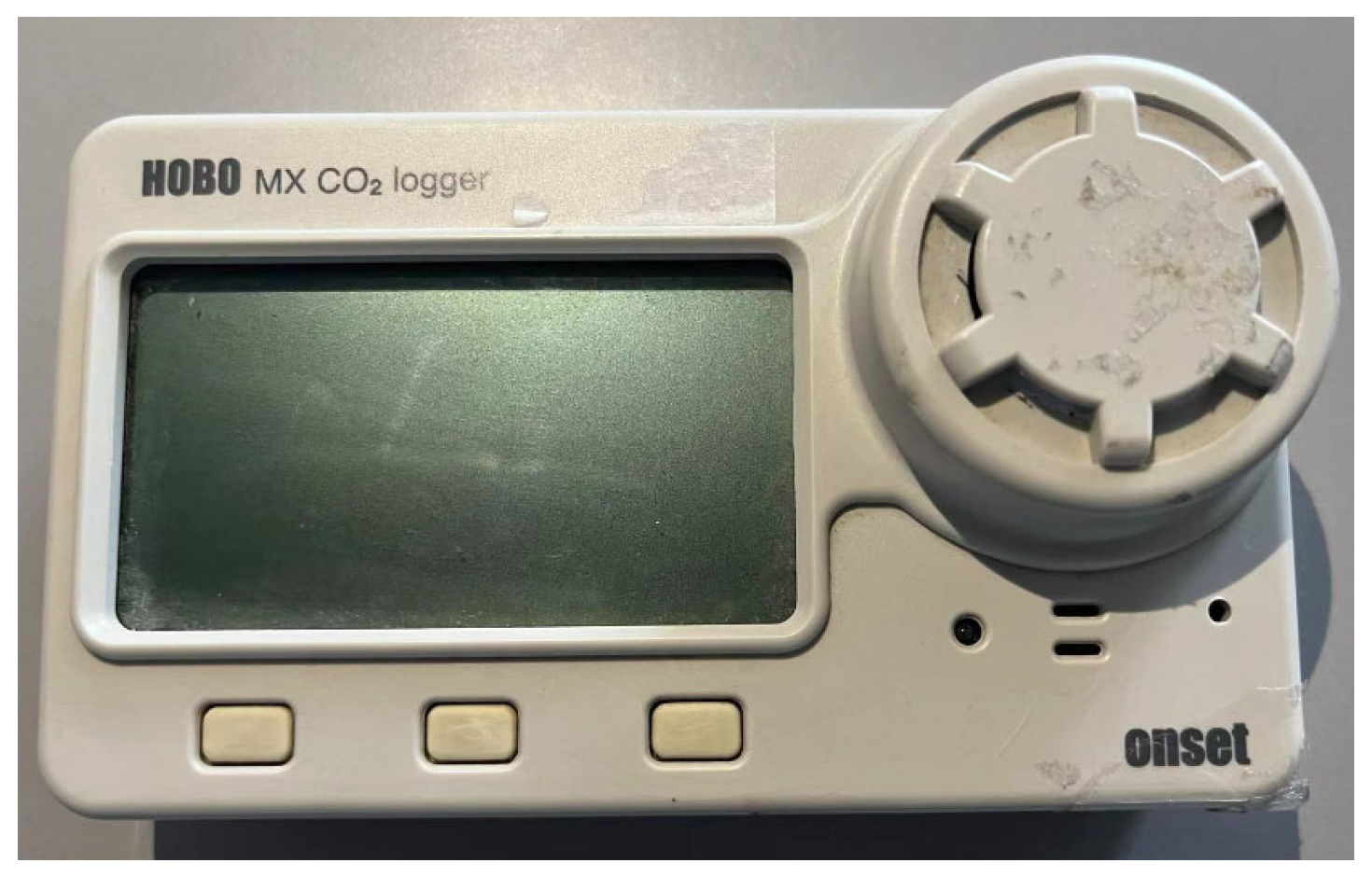
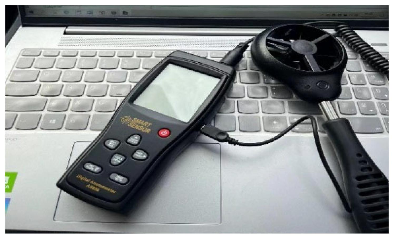
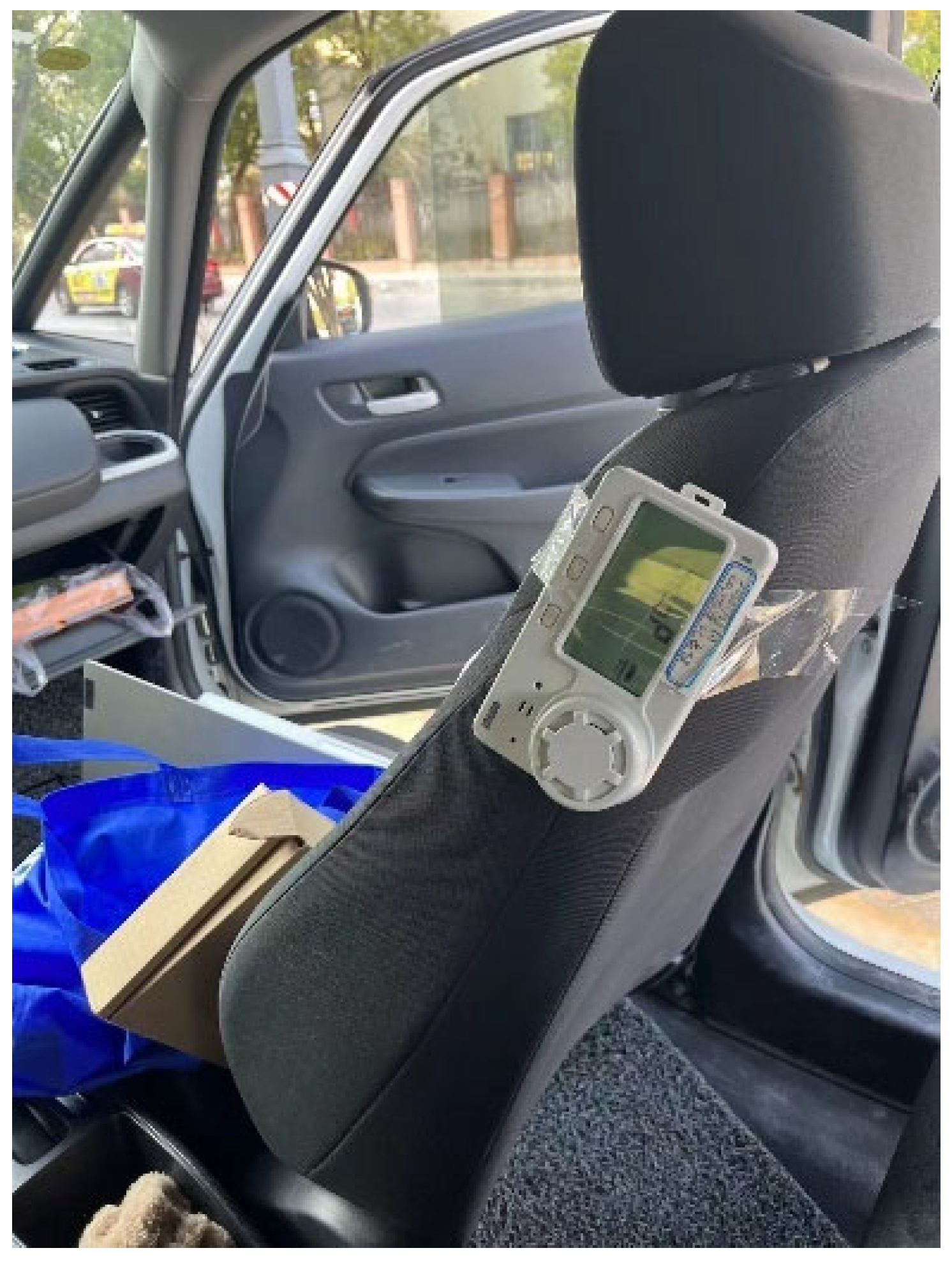
2.1.1. Test Subjects and Instrument Layout

The two test vehicles used in this research were common 1.5 L 5-seater family vehicles, namely, the Nissan-Sylphy and Honda-Fit. Both gasoline-powered vehicles use Euro VI 92. Table 3 presents detailed information about these vehicles. The data on the concentration of CO2, temperature, and humidity in the vehicle were collected using a HOBO tester (Figure 1), and fan speed at the air outlet was measured using a smart sensor anemometer (Figure 2). Instrument parameters are provided in Table 4. The study utilized mobile phone software capable of satellite connectivity to record real-time vehicle speed; the software is based on the Android platform. To avoid the impact of occupant respiration and solar radiation on data recording, the instrument is positioned at the center of the vehicle, aligned with the right shoulder height of the front row. The location of the testing device is illustrated in Figure 3. A total of three occupants participated in this field test, with one occupant seated on the right side of the front row, another on the left side of the rear row, and a designated driver included. The participants in this field test were exclusively male. The weight, height, and age of the participants were strictly controlled to fall within the ranges of 65–70 kg, 165–170 cm, and 24–26 years old, respectively, in order to minimize the impact of weight, body composition, sex, and other physiological factors on CO2 exhalation levels. Additionally, none of the three subjects engaged in strenuous physical activity prior to testing.

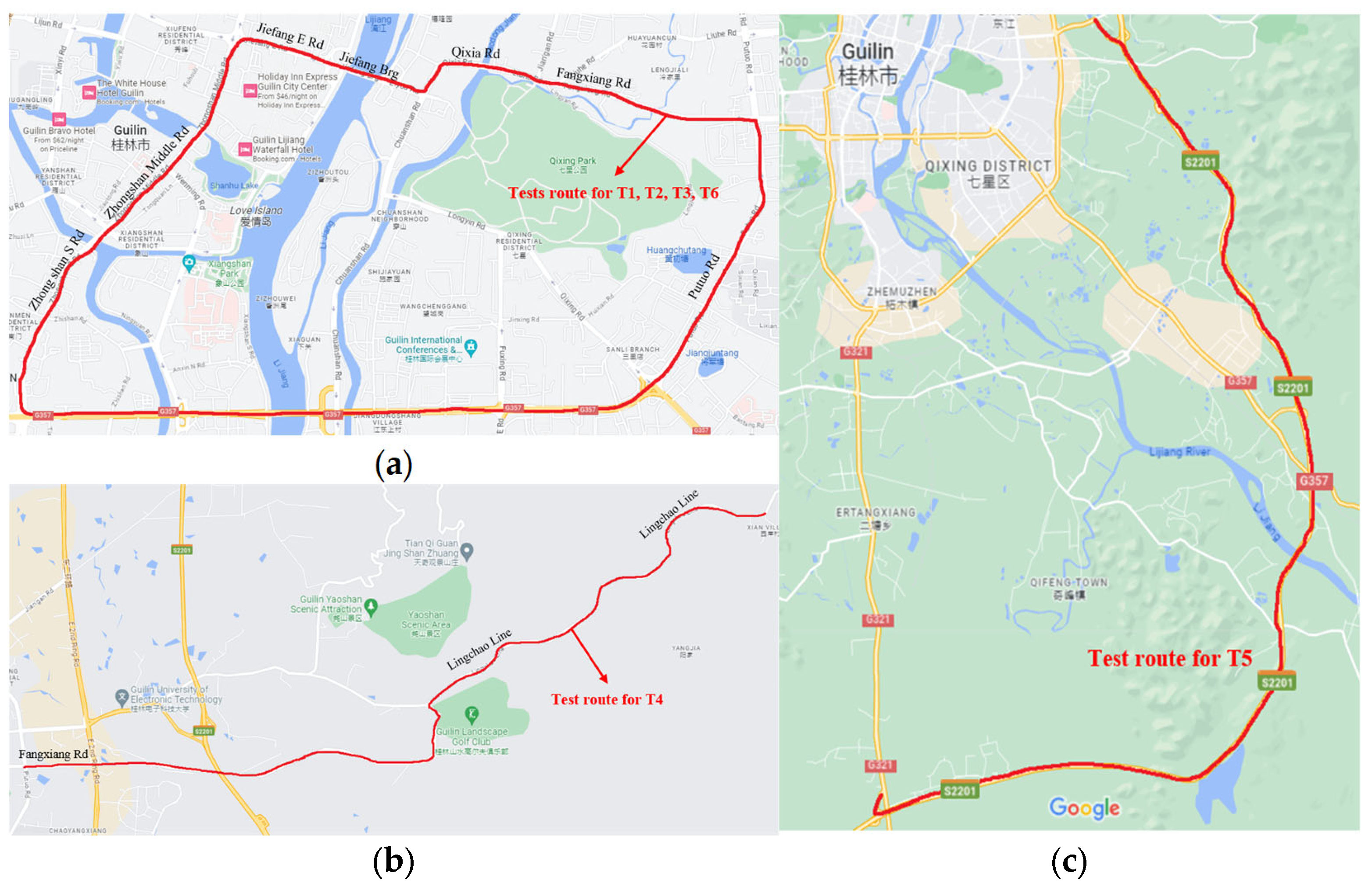
2.1.2. Test Location and Process

The field test site was situated in Guilin, Guangxi, and the test was conducted on 14–15 December 2022, under clear weather conditions. Given that the concentration of CO2 inside a vehicle is influenced by various factors such as ventilation settings, the number of occupants, driving speed, and vehicle characteristics [13,14], this research monitored changes in CO2 concentration across these different variables. We conducted a total of six field tests, and the specific operational conditions during each test are presented in Table 5. T1–T2 were designed to monitor and compare the impact of varying fan speeds on the rate of CO2 increase. The fan speed of the Nissan-Sylphy is categorized into seven different levels. We selected level 1 (S1) and level 4 (S4) for the purpose of testing. The fan speeds at the vents of S1 and S4 were measured as 0.756 m/s and 1.648 m/s, respectively. The purpose of T3 and T1 is to monitor and compare the impact of varying numbers of passengers on the rate of CO2 increase. T4–T5 were designed to monitor and compare the impact of varying vehicle speeds on the rate of CO2 increase. T1–T5 were conducted in a Nissan-Sylphy, and T6 in a Honda-Fit to assess the effect of different interior spaces on the rate of increase in CO2. The S1 fan speed at the air vent of the Honda-Fit was measured to be 0.723 m/s, which is approximately equivalent to that of the Nissan-Sylphy. The reference data for this research were obtained from the T1 test results, with all other tests compared against it. Our field test design refers to the test methodology described in reference 14.
We selected three driving routes: 12 km of urban roads, with a speed range of 0–40 km/h; 15 km of suburban roads, with a speed range of 0–80 km/h; and 28 km of highways, with a speed range of 60–120 km/h. The duration for each test was controlled at 20 min, and the driving route is illustrated in Figure 4. During the test, the windows were closed, and the air conditioning system was set to internal circulation mode. Prior to each experiment, the instrument underwent calibration in an outdoor open area. Subsequently, fresh air was introduced into the vehicle by opening its doors and windows until the CO2 concentration inside reached an equilibrium with that of its surroundings. Only then did all personnel enter the vehicle and commence testing. Each measurement lasted for a duration of 20 min, during which data were recorded at intervals of 5 s, resulting in a total collection of 1440 sets of data.

2.2. Prediction Models

This research utilizes the ARIMA model and LSTM model to predict in-vehicle CO2 concentration. Specifically, it aims to identify regularity among the previous moment data (t0, t1, t2, …, tn−1, tn) and to predict the subsequent moment data (tn+1). The research was implemented using Python 3.8 for modeling and simulation in order to achieve accurate predictions of in-vehicle CO2 concentration changes.

2.2.1. ARIMA Model

The ARIMA model is a statistical model that combines autoregressive (AR) and moving average (MA) models to predict stochastic time series data. It was first proposed by Box, an American researcher, and Jenkins, a British statistical researcher, in the 1970s [67]. The model identifies intrinsic relationships between historical and current values to forecast future data.
The AR model is based on a mathematical equation to describe the autocorrelation in a time series, i.e., the relationship between the current moment (t) and the previous moment (p) values. The autoregressive model of order p is denoted as AR(p) and is expressed as shown in Equation (1):
Y t = c + α 1 Y t 1 + α 2 Y t 2 + α 3 Y t 3 + + α p Y t p + ε t
The MA model is known as a moving average model and represents a weighted average sum of several white noises. The q–th order moving average model is denoted as MA(q), as shown in Equation (2):
Y t = β 1 ε t 1 β 2 ε t 2 β 3 ε t 3 β q ε t q + ε t
Combining the AR model with the MA model yields the ARMA model, as shown in Equation (3):
Y t = c + α 1 Y t 1 + α 2 Y t 2 + α 3 Y t 3 + + α p Y t p + ε t β 1 ε t 1 β 2 ε t 2 β 3 ε t 3 β q ε t q
The ARIMA model is the model calculated by differencing the data d times using the ARMA model, denoted as ARIMA (p, d, q). The ARIMA model is used for time series forecasting in the following steps:
  • Data stationarity analysis: Prior to establishing an ARIMA prediction model, it is imperative to evaluate the stationarity of the data. The augmented Dickey–Fuller test (ADF) is employed to estimate whether the data are stationary or not in this research. If the data exhibit stability, the significance p-value should be less than 0.05; otherwise, differencing must be applied to non-stationary data until they achieve stationarity.
  • Estimation of model hyperparameters: The stationary time series data are further processed to obtain the autocorrelation coefficient (ACF) and partial autocorrelation coefficient (PACF). After determining the range of hyperparameters p and q, it is necessary to continuously try to determine the combination of model hyperparameters with the highest accuracy, but this method has an interference of certain human factors. Therefore, the “auto. arima” function in Python can be utilized to automatically determine the optimal combination of hyperparameters, selecting the optimal model by means of the Akaike Information Criterion (AIC) and Bayesian Information Criterion (BIC), thereby eliminating any potential influence from human factors during the selection process. The range of AIC and BIC values is not fixed but varies across different datasets. Usually, the combination of hyperparameter p and q that yields the smallest AIC and BIC values represents the most suitable model. The calculation method for AIC and BIC is shown in Equations (4) and (5):
AIC = 2 k 2 l n ( L )
BIC = k l n ( n ) 2 l n ( L )
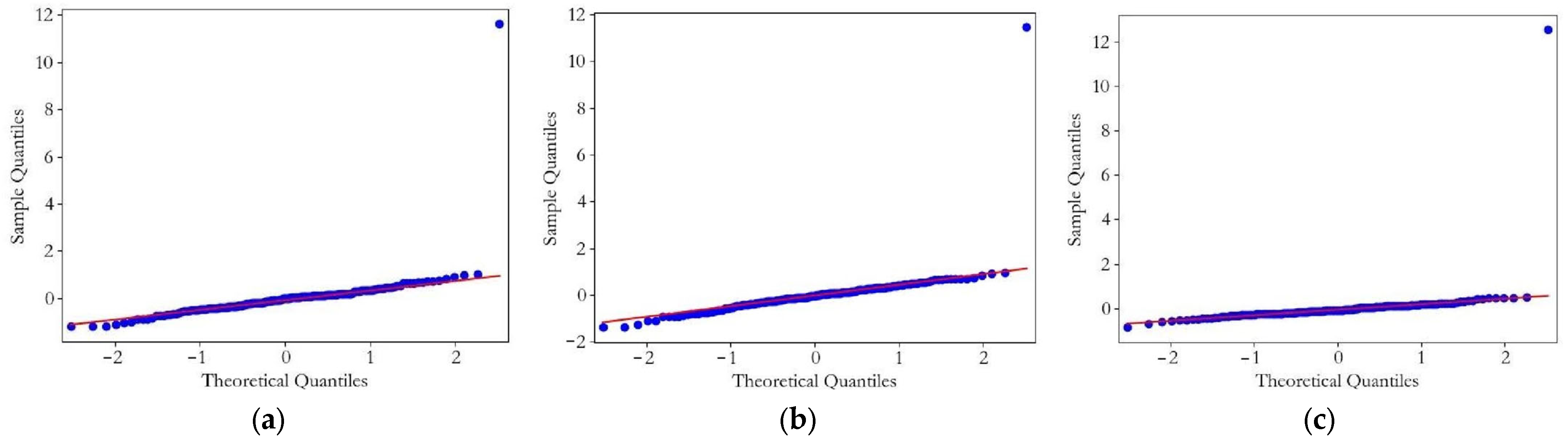
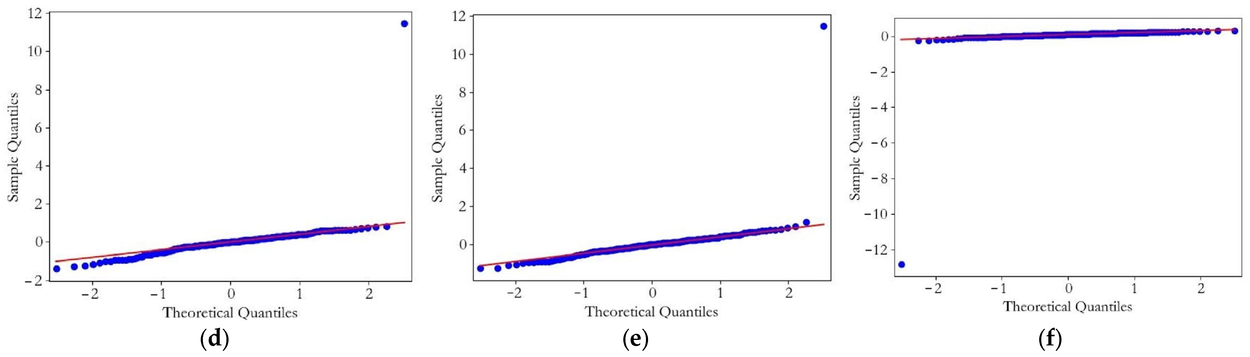
  • Test the validity of the optimal model: Before forecasting, the effectiveness of the optimal model needs to be tested. Firstly, the Ljung–Box test method is used to judge whether the residual of the prediction model is a white noise sequence. If p-value > 0.05, it can be considered that the residual is a white noise sequence. Then, the Q test is used to check the normal distribution of the model residuals, and a Q–Q diagram is drawn to observe the distribution of the residuals.
  • Forecast the data: After completing the aforementioned actions, predictions can be made.
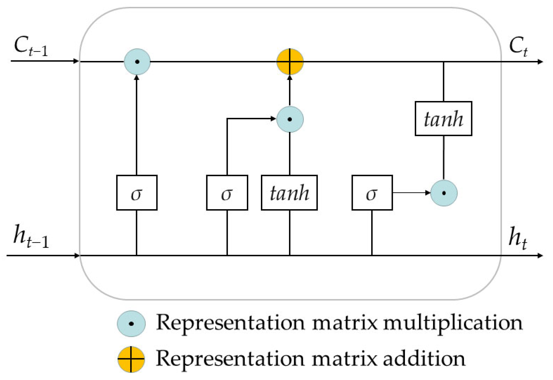
2.2.2. LSTM Model

In 1997, Sepp Hochreiter and Jurgen Schmidhuber proposed the LSTM neural network [68], which is an improved version of a recurrent neural network (RNN). The single-cell structure of the LSTM cell structure is shown in Figure 5, with each cell having three gates: the “input gate”, the “forget gate”, and the “output gate”. This “gate” can be opened or closed to determine whether the output of the memory state (the previous state of the network) of the model neural network reaches a threshold value at that layer, so that it can be added to the current calculation of that layer [69]. Each gating unit is a sigmoid activation function that controls the flow of information. In the LSTM model, each time step has a hidden state ht and a cell state Ct. Cell states are a central part of the LSTM model, which allows the neural network to selectively forget or preserve information. The cell state Ct at each time step depends on the cell state Ct−1 at the previous time step, the input xt at the current time step, and the output of the gating unit. LSTM’s cell states can pass information between multiple time steps, allowing the neural network to capture long-term dependencies. It is possible to keep the important information and forget the minor information, to be able to identify the regular changes in time series data, and to realize the prediction. The training process of the LSTM neural network uses a back propagation algorithm combined with gradient cropping to address the shortcomings of traditional recurrent neural network gradient explosion.
The mathematical formulations for the input gate (it), forgetting gate (ft), and output gate (ot) are presented in Equations (6)–(8). The memory cell C is utilized for the storage and transmission of long-term information within the network, with mathematical expressions depicted in Equations (9) and (10). Equation (11) depicts the output ht generated by the LSTM network:
i t = σ ( W i [ h t 1 , x t + b i ] )
f t = σ ( W f [ h t 1 , x t ] + b f )
o t = σ ( W o h t 1 , x t + b o )
C t = f t C t 1 + i t C t
C t = t a n h ( W c [ h t , x t ] + b c )
h t = o t t a n h ( C t )
The key steps for time series prediction using LSTM are as follows:
  • Data preprocessing: Data preprocessing can effectively reduce noise, eliminate redundant information, and extract key features from data to enhance the training and prediction performance of neural network models. This research employs the max-min normalization method for data preprocessing. This process ensures that all data values are reflected within the [0, 1] interval. The calculation method for normalization is as follows:
y i = x i min ( x i ) max ( x i ) min ( x i )
  • Determining the neural network structure: Determine the inputs and outputs of the neural network and the number of neurons in the hidden layer.
  • Network training: Determine the loss function, activation function, optimizer, and other parameters utilized for training the LSTM network. The loss function adopts the mean squared error (MSE) as the criterion for evaluation. The computation of the MSE is illustrated below:
MSE = 1 n i = 1 n ( y i y i ^ ) 2
MSE, which stands for mean squared error, is a metric used to assess the accuracy of a model’s predictions. It is calculated by averaging the squared differences between the predicted and true values. The activation functions use the sigmoid function. The adaptive moment estimation (Adam) was selected as the optimizer for this research. The Adam optimizer is suitable for problems where the gradient is sparse or noisy. The update of its parameters is not affected by the gradient scaling transformation. It is a commonly used optimizer for deep learning.
  • Make predictions: After the aforementioned steps have been completed, the trained model can be utilized for predictions.

2.3. Evaluation Indicators

The model forecasts are evaluated for accuracy using MAPE and RMSE, which are calculated as shown below:
MAPE = 100 % n i = 1 n y ^ i y i y i
RMSE = 1 n i = 1 n y ^ i y i 2

3. Results

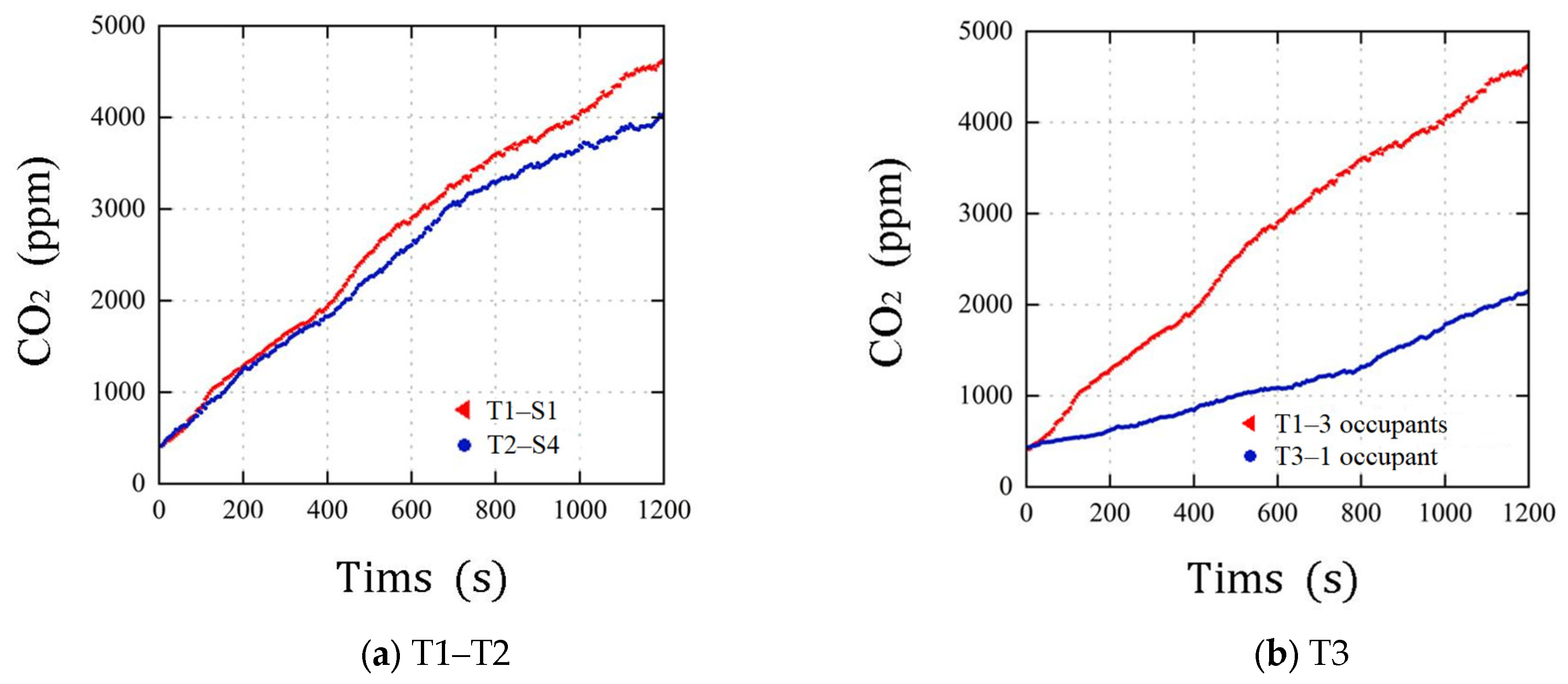
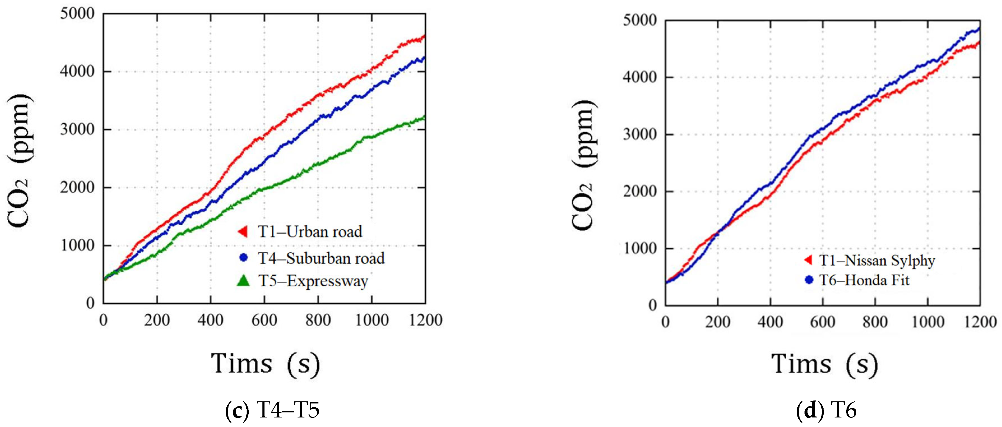
3.1. Analysis of In-Vehicle CO2 Concentration

The mean values of temperature, humidity, CO2 concentration, and rate of CO2 increase during the six field tests are presented in Table 6. Temperature and humidity remained relatively stable due to the operation of the vehicle’s air conditioning system. The CO2 concentration measurements for each field test are presented in Figure 6. During testing, the windows were closed, and internal circulation was activated, resulting in an increase in the CO2 concentration over time. Due to real-time changes in vehicle speed causing an unstable air change rate, there were fluctuations observed during the growth process of CO2 concentrations, similar to the field test results from Luangprasert et al., Lohani et al., and Zhao et al. [6,13,28]. The impact of different fan speeds on the increase in the in-vehicle CO2 concentration is illustrated in Figure 6a. After 20 min, the CO2 concentration levels exceeded 4000 ppm in T1–S1 and T2–S4, with rates of CO2 increase of 3.52 ppm/s and 3.02 ppm/s, respectively. The higher air speed at the air conditioning outlet in S4 results in an increased frequency of air exchange between the cabin and its surrounding environment, leading to a lower rate of CO2 increase. The impact of different numbers of occupants on the increase in the in-vehicle CO2 concentration is illustrated in Figure 6b. With three occupants, the CO2 concentration reaches 4633 ppm after 20 min, exhibiting a rate of CO2 increase of 3.52 ppm/s. With one occupant, the CO2 concentration increases to 2152 ppm at a rate of 1.43 ppm/s after 20 min. The comparison indicates that with three occupants in the vehicle, the CO2 concentration attained after 20 min is 2.53 times higher than that with only one occupant, and the rate of CO2 increase is 3.03 times greater. Figure 6c illustrates the rate of CO2 increase within a vehicle at varying driving speeds. Disregarding the impact of road conditions, when traveling at an average speed of 85.89 km/h on an expressway, the CO2 concentration reaches 3176 ppm after 20 min, with a rate of CO2 increase of 2.30 ppm/s. When traveling at an average speed of 55.85 km/h on a suburban road, the CO2 concentration reaches 4228 ppm, with a rate of CO2 increase of 3.17 ppm/s after 20 min of driving. The test data showed that a lower rate of CO2 increase will be caused by increasing driving speed, and a lower concentration level will be reached over the same period. The phenomenon can be attributed to the reason that as the speed of driving increases, so does the external dynamic pressure. The static pressure decreases, and the leakage of air from the inside to the outside of the vehicle is accelerated, resulting in a reduction in the rate of CO2 increase. The impact of different interior vehicle volumes on the increase in the in-vehicle CO2 concentration is illustrated in Figure 6d. The T6–Honda Fit exhibits a CO2 concentration of 4870 ppm after 20 min, with a rate of CO2 increase of 3.72 ppm/s. Compared to the T1–Nissan Sylphy, which reaches 4633 ppm of CO2 concentration after 20 min, the concentration of the Nissan-Sylphy is 237 ppm smaller than that of the Honda-Fit. Since the interior space of the Nissan-Sylphy is 0.3 m3 larger than that of the Fit, the calculation shows that each 1 m3 increase in the volume of the vehicle reduces the CO2 concentration by 790 ppm.
The majority of indoor CO2 concentration standards, as summarized in the preceding introduction section, are set at 1000 ppm. Hudda and Fruin [22] indicated a concentration threshold of 2500 ppm for automotive CO2 concentrations, above which negative effects can occur. Therefore, we used 1000 ppm and 2500 ppm as the evaluation criteria. From the test data, it is found that the rate of CO2 increase in the vehicle is rapid when the RC ventilation mode is turned on. When there are three occupants in the vehicle, the rate of CO2 increase for the T6–Honda Fit artificial condition is the fastest, reaching 1000 ppm in 160 s (about 2.5 min) and 2500 ppm in 470 s (about 8 min); the T3–1 artificial condition has the slowest rate of CO2 increase, reaching 1000 ppm within 500 s (about 8 min). The CO2 concentration reached 1000 ppm within a range of 120–245 s during the T1–S1, T2–S2, T4–suburban road, and T5–expressway tests. The average concentration within 20 min of the six groups of working conditions all exceeded 1000 ppm, and the T1–S1, T6–Honda Fit working conditions even exceeded 2500 ppm, with the proportion of time exceeding 2500 ppm in the test process exceeding 59%. CO2 concentration is a key indicator for judging the degree of ventilation in a vehicle [13]. Therefore, when the windows are closed, and internal air circulation is activated, the concentration of CO2 can easily exceed safe levels, posing a potential hazard to driving safety. A timely increase in ventilation is necessary to reduce the in-vehicle CO2 concentration.

3.2. Fitting Models and Prediction Result Analysis

3.2.1. ARIMA Model

Using the ADF test to all datasets revealed a p-value exceeding 0.05, meaning that all datasets are non-stationary, meaning that the data required differencing. The ADF test is applied again after all data are first differenced, and the test results are shown in Table 7. The p-value is lower than the significance level of 0.05, and the t statistic is smaller than 1%, 5%, and 10%. The null hypothesis of non-stationarity in the time series should be rejected. It is indicated that the data after difference have been stabilized, and the mean and variance do not change with time, which meets the prerequisites for forecasting using the ARIMA model. Therefore, we set the order of difference d = 1 for all the datasets.
Table 8 displays the AIC and BIC values corresponding to the optimal model hyperparameter combinations and the significance p-values after the Ljung–Box test. The p-values of the six models are greater than 0.05, indicating that the prediction residuals of the models conform to a sequence of random numbers and support the assumption that they are white noise.
Figure 7 shows the Q–Q plots of predicted residuals for six optimal models. The x-axis in the Q–Q graph represents the quantile of the theoretical distribution, the y-axis represents the quantile of the model prediction residual, the red straight line is the normal distribution line, and the solid blue dot is the model prediction residual value. The closer the solid blue dot is to the red straight line, the more it conforms to the standard normal distribution. It can be seen from the figure that most of the solid blue dots are located on the red straight line, indicating that the predicted residual values of the best model obey the normal distribution. To conclude, the residuals satisfy the requirements of a white noise sequence and conform to a normal distribution. Therefore, the model is suitable for prediction.

3.2.2. LSTM Model

After multiple attempts, the following LSTM network structure settings were used for CO2 concentration prediction:
  • Input layer: After continuous debugging of the size of the time window, it was found that the error is the smallest when the number of time windows is three. Therefore, the neuron dimension of three has been selected for our input layer.
  • Output layer: Since our goal is to forecast CO2 concentration for future moments, the number of neurons in the output layer is therefore determined to be one.
  • Hidden layer: In this research, we utilized a sequential model in Keras, which is comprised of one LSTM layer and one dense layer. The neuron dimension of the first hidden layer is 64, and the second hidden layer has a neuron dimension of 1.
Therefore, this research chose three as the number of neurons in the input layer, namely, Xt = f (Xt−1, Xt−2, Xt−3). This is utilizing the preceding three data points to forecast the next one data point. The other parameters are configured as follows: The learning rate is set to 0.002. The maximum number of iterations (epoch) is set to 200, and the number of samples passed to the model for training each time (batch size) is 32. This network architecture exhibits the lowest RMSE and is well suited for predicting CO2 concentration.
In summary, the final model structure of the LSTM neural network is as follows:
The neuron dimension of the input layer is three, and the neuron dimension of the output layer is one. It consists of a LSTM layer and a dense layer. The neuron dimension of the LSTM layer is 64, and the neuron dimension of the dense layer is 1. The optimizer chosen is Adam. The learning rate is set to 0.002. The epoch is set to 200, and the batch size is 32. This model has the smallest error, a high fitting degree, and high prediction accuracy, so this structure is used for prediction.

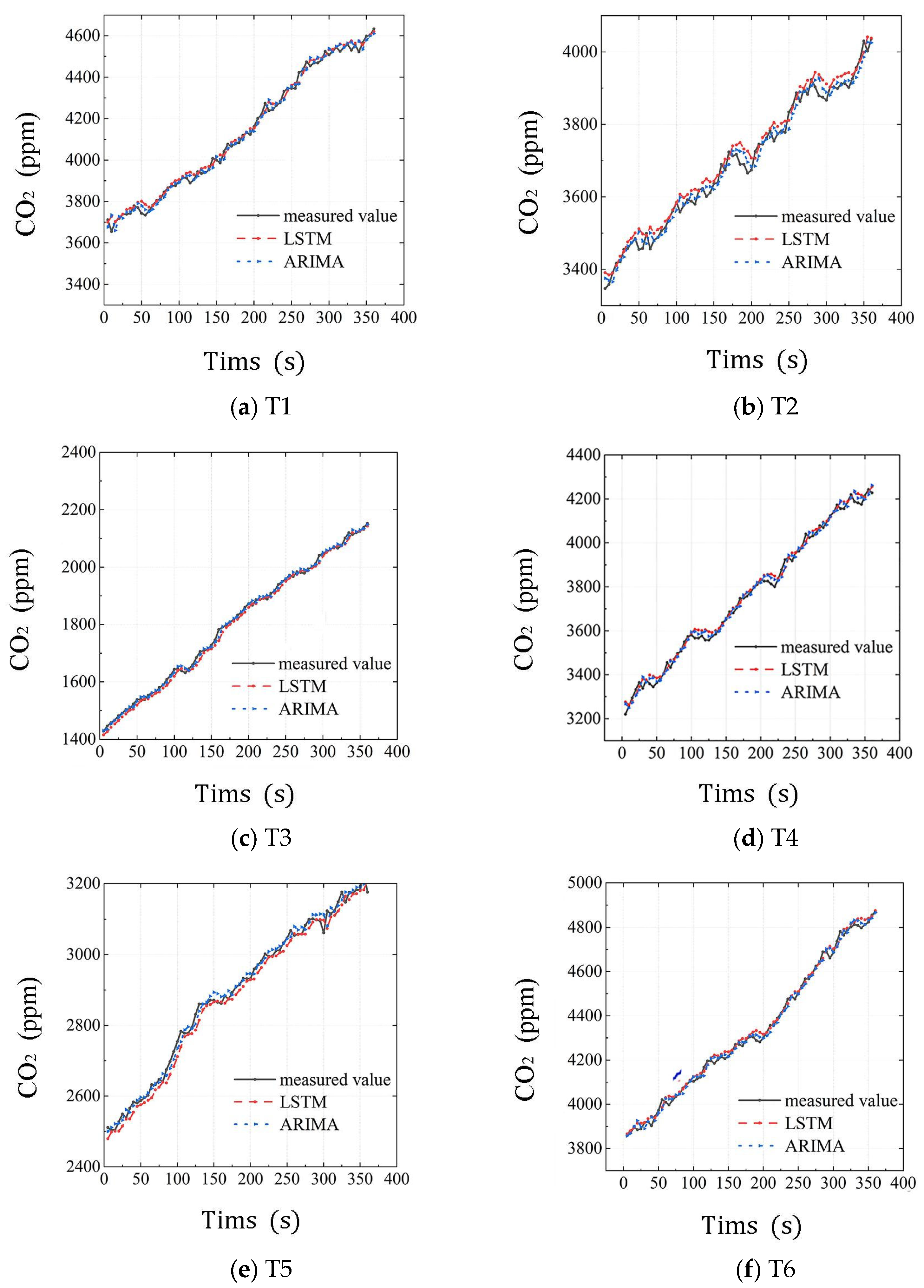
3.2.3. Results of Model Predictions and Comparative Analysis

The duration of each field test is 1200 s (20 min), with a data collection interval of 5 s. A total of 240 sets of data were collected in each test, which are then divided into training and testing sets at a seven-to-three ratio to evaluate the predictive performance of two models—ARIMA and LSTM. Figure 8 illustrates the comparison between predicted values and actual values for both models. The two models effectively learned the regular patterns in the historical data and are capable of accurately predicting variations in CO2 concentration under different fan speeds, occupancy levels, driving speeds, and vehicle volumes. Furthermore, their prediction curves closely align with the actual value curves, obtaining an accurate prediction result. The prediction results demonstrate the accuracy and good generalization ability of both models in predicting changes in CO2 concentration within a vehicle, effectively capturing fluctuations during driving. The predicted curve closely aligns with the actual curve and exhibits excellent fitting effects. The two models are capable of forecasting variations in CO2 concentration across diverse vehicle models and driving scenarios. However, in terms of the prediction results for the T2, T3, and T5 datasets, the ARIMA prediction curves show a closer alignment with the actual values compared to LSTM.
The RMSE and MAE values for the prediction results of both models are presented in Table 9. The ARIMA model exhibits superior performance, with an average MAPE of 0.46% and RMSE of 19.62 ppm, respectively, compared to the LSTM model’s values of 0.56% and 22.76 ppm. The MAPE metric reflects the accuracy of the model’s predictions, and the RMSE metric measures the average deviation between predicted and true values. Lower values indicate better performance. The ARIMA model exhibits lower MAPE and RMSE values compared to the LSTM model, indicating superior prediction accuracy in forecasting CO2 concentration changes within a vehicle. And the degree of deviation between the predicted value of ARIMA and the true value is also lower than that of LSTM.

4. Discussion

The CO2 concentration in vehicles is affected by factors such as ventilation settings, the number of passengers, driving speed, vehicle characteristics, etc. There are many influencing factors, and they are coupled with each other. Parameters such as the amount of air leakage in a vehicle are difficult to obtain [27], and the accuracy of the model needs to be calibrated with data from multiple studies [13]. Therefore, the utilization of conventional mathematical models for computations encounters certain challenges. When utilizing ARIMA and LSTM for prediction, it is not necessary to deeply explore the impact of various influencing factors on CO2 concentration. Instead, future trends can be predicted by capturing historical data and analyzing its correlation, seasonal and periodic fluctuations, as well as noise characteristics, leading to accurate prediction results. Additionally, ARIMA and LSTM have demonstrated their reliability in accurately predicting unconventional fluctuations in data [60]. In this research, we utilized ARIMA and LSTM models to build a predictive model for in-vehicle CO2 concentrations, which yielded accurate forecast results. Predicting in-vehicle CO2 levels can assist in maintaining a favorable in-vehicle environment, improving traffic safety, and enhancing driving comfort. Lohani et al. [28] employed the ARIMA (0, 1, 0) model to forecast the variation in the CO2 concentration in a vehicle, yielding MAPE and RMSE values of 3.79% and 55.32 ppm, respectively. Compared to this result, the ARIMA model employed in our research yielded more precise prediction outcomes, which may indicate that our model, which considers the autoregressive and moving average items, can better capture the correlations and trends in historical data, whereas ARIMA (0, 1, 0) only performs differential processing on the data and does not consider the correlation with historical data.
The prediction principle of ARIMA is to filter the high-frequency noise in the data, detect the linear correlation in the historical data, and use this correlation to predict the future development trend. The prediction principle of RNN involves combining the current input with the previous hidden state to establish temporal dependencies in time series data, which can capture nonlinear relationships within the data. LSTM builds upon this by introducing gating mechanisms that enable memory cells to retain relevant information over longer periods of time, making it particularly effective for large datasets and mitigating issues related to vanishing gradients in traditional RNNs. In our research, the predictive accuracy of LSTM was inferior to that of ARIMA. The possible reasons contributing to this outcome are as follows: (1) The linear relationship of in-vehicle CO2 concentration data is strong, and there is a clear upward trend in the concentration. ARIMA effectively captures the linear law within time series data, whereas LSTM excels at predicting complex nonlinear patterns. (2) The in-vehicle CO2 concentration is a one-dimensional time series form of data. Due to the rapid growth process, the amount of data collected at intervals of 5 s within 20 min is only 240 sets. The learning ability of LSTM is restricted by the insufficient amount of data. When predicting data with a limited number of samples and only one dimension, the prediction accuracy of ARIMA may surpass that of LSTM. LSTM requires a large amount of data for training, and the larger the training volume, the higher the prediction accuracy of LSTM. Therefore, using LSTM has a better effect when predicting datasets with a large amount of data [46]. Even though LSTM’s prediction accuracy is somewhat lower than that of ARIMA, it still has numerous advantages as a deep-learning model compared to ARIMA. Firstly, the process of utilizing ARIMA prediction is more intricate than that of LSTM. It involves a series of steps such as time series stabilization detection, model order determination, and validity inspection. In contrast, LSTM can detect regularity in raw data without any mathematical processing, making the prediction process more convenient. Secondly, the use of ARIMA prediction must ensure that the data are stationary. Not all data can be stable after differencing processing, and the data may lose important information after differencing processing, which means that ARIMA may not be able to achieve good results when predicting certain types of data. However, LSTM can be used for non-stationary data prediction. Finally, due to its memory units and gating mechanisms, LSTM is capable of predicting complex multivariate nonlinear data, whereas ARIMA, being a linear model, falls short in this regard. The non-linear nature of the changes in data renders ARIMA incapable of producing accurate predictions for complex multivariate time series data [62], which demonstrates the broader applicability of LSTM. Furthermore, both models have their respective shortcomings. The ARIMA model is not well suited for analyzing data with long-term dependencies, and its predictive capability for nonlinear data is limited. The model’s predictive performance tends to degrade when handling large datasets. On the other hand, LSTM models involve a significant number of hyperparameters that require tuning. They are computationally expensive and demand considerable computational resources compared to simpler models like ARIMA.
From the comparative research of the two models, it is found that machine learning is not superior to traditional statistical models in all cases, and it is necessary to select an appropriate prediction model according to the amount of data. When the amount of data used for training reaches 1000, LSTM shows better predictive performance [57,58,70,71,72]. Both of these two models have their advantages when the amount of training data is between 100 and 1000 [44,45,71,72,73,74,75]. ARIMA exhibits better accuracy when the amount of training data is less than 100 [59,60,76,77]. In addition, although our research focuses on the in-vehicle CO2 concentration in a Nissan-Sylphy and a Honda-Fit under the driving conditions outlined in Table 3, the prediction method used is also applicable to the prediction of CO2 concentration changes in different vehicles under other driving conditions.
The research findings can provide a theoretical foundation for the development of more complex prediction models in the future and serve as crucial evidence for establishing a CO2 concentration prediction model within the traffic safety management system. However, this research also has several limitations. Firstly, our anemometer lacks the capability to record airflow data. Secondly, our prediction model solely relies on historical data for forecasting future trends, without considering influential factors or elucidating the underlying mechanisms. Therefore, forthcoming research should incorporate influential factors and establish multivariable time series prediction models.

5. Conclusions and Future Work

This research focuses on the concentration of CO2 in vehicles as its research subject. Through field tests, data on the CO2 concentration within vehicles were obtained and established using both ARIMA and LSTM prediction models for forecasting changes in CO2 concentration. The accuracy of these two models was analyzed and compared, with differences in performance discussed. The main conclusions are as follows:
  • The measured data indicate that with closed vehicle windows and internal circulation turned on, the concentration of CO2 in a vehicle increases proportionally to driving time. Under all test conditions, the average CO2 concentration within 20 min exceeds the standard limit of 1000 ppm. During driving, it is necessary to improve vehicle ventilation by opening windows, switching to outside air mode, and using other methods.
  • Both the ARIMA and LSTM models are capable of accurately predicting changes in the CO2 concentration within a vehicle. However, the MAPE and RMSE values obtained from the ARIMA model’s predictions are lower than those produced by the LSTM model. Therefore, the ARIMA model is more accurate in predicting changes in the CO2 concentration within a vehicle compared to the LSTM model.
  • The prediction performance of LSTM is not always better than the ARIMA model, and the two models need to be selected according to the characteristics of the data. When the amount of data used for training reaches 1000, it is better to use LSTM, and it is more appropriate to use ARIMA when the amount of data is within 100, but comparative analysis is required when the amount of data is within 100–1000.
Predicting the change in CO2 can remind the people in a vehicle to take control measures before the concentration exceeds the standard. This research provides a critical theoretical basis for the future selection of early warning prediction models for in-vehicle CO2 concentrations and for establishing efficient in-vehicle ventilation control systems.
In future research, we should develop an in-vehicle ventilation management system that integrates predictive capabilities with control functionalities. Furthermore, we should comprehensively consider the influencing factors of in-vehicle CO2 concentration and develop a time series prediction model that incorporates multiple input variables to investigate whether these models can provide more accurate predictions of in-vehicle CO2 concentration.

Author Contributions

Supervision, conceptualization, methodology, writing—review, J.H.; design and conducting of experiments, original draft, H.L.; algorithm implementation, writing—review and editing, Z.Q. All authors have read and agreed to the published version of the manuscript.

Funding

Thanks to the Guangxi Natural Science Foundation’s “Study on the thermal adaptation behavior characteristics of opening/closing windows and turning on/off air conditioners of mixed cooling building residents in Guangxi area” (Funder: Associate Prof. Jie Han, Funding number: 2018GXNSFAA281212) and Guangxi Public Security Department Research Project “Research on the Construction of Knowledge Graph in the Field of Telecom Fraud” (Funder: Senior Engineer. Zhenkai Qin, Funding number: 2023GAZD018) for their support of this research.

Institutional Review Board Statement

Not applicable.

Informed Consent Statement

Not applicable.

Data Availability Statement

Not applicable.

Conflicts of Interest

The authors declare no conflict of interest.

Nomenclature

cConstant
pp–order of autoregressive model
YtTime series
α1, α2, α3, …, αpAutoregressive coefficient
εtWhite noise sequence (uncorrelated with the previous moment value)
qq–order of moving average
β1, β2, β3, …, βqThe moving average coefficient
dThe number of differencing required to achieve stationarity in the data
kThe number of model parameters
nSample size
LLikelihood function
xtThe input value of the network at the current moment
ht−1The output value of the LSTM at the previous moment
[ht−1, xt]The two vectors are joined to form a longer vector
WoWeight
boBias term
σSigmoid function
ftThe output value of the forget gate
Ct−1The state of the unit at the previous moment
CtThe state of the unit at the current moment
C t The updated value of the input gate
tanhTanh activation function
min(xi)The minimum value of the i–th attribute in x
max(xi)The maximum value of the i–th attribute in x
yiMeasured value
ŷiPredicted value
air change rateThe rate at which air is exchanged between the enclosed environment and the surrounding environment
air leakageThe uncontrolled exchange of air between in-vehicle environment and the external environment

References

  1. Gladyszewska-Fiedoruk, K. Concentrations of carbon dioxide in a car. Transp. Res. Part D Transp. Environ. 2011, 16, 166–171. [Google Scholar] [CrossRef]
  2. Jones, A.P. Indoor air quality and health. Atmos. Environ. 1999, 33, 4535–4564. [Google Scholar] [CrossRef]
  3. ASHRAE. Position Document on Indoor Air Quality. Available online: https://www.ashrae.org/file%20library/about/position%20documents/pd_indoor-air-quality-2020-07-01.pdf (accessed on 18 September 2023).
  4. Jayasankar, P.; Subbaian, J. Optimization of in-Vehicle Carbon Dioxide Level in a 5-Seat Car. Strojniški Vestnik J. Mech. Eng. 2022, 68, 471–484. [Google Scholar] [CrossRef]
  5. Lim, S.; Mudway, I.; Molden, N.; Holland, J.; Barratt, B. Identifying trends in ultrafine particle infiltration and carbon dioxide ventilation in 92 vehicle models. Sci. Total Environ. 2022, 812, 152521. [Google Scholar] [CrossRef]
  6. Luangprasert, M.; Vasithamrong, C.; Pongratananukul, S.; Chantranuwathana, S.; Pumrin, S.; De Silva, I. In-vehicle carbon dioxide concentration in commuting cars in Bangkok, Thailand. J. Air Waste Manag. Assoc. 2017, 67, 623–633. [Google Scholar] [CrossRef]
  7. Tolis, E.I.; Karanotas, T.; Svolakis, G.; Panaras, G.; Bartzis, J.G. Air quality in cabin environment of different passenger cars: Effect of car usage, fuel type and ventilation/infiltration conditions. Environ. Sci. Pollut. Res. 2021, 28, 51232–51241. [Google Scholar] [CrossRef]
  8. Moreno, T.; Pacitto, A.; Fernández, A.; Amato, F.; Marco, E.; Grimalt, J.O.; Buonanno, G.; Querol, X. Vehicle interior air quality conditions when travelling by taxi. Environ. Res. 2019, 172, 529–542. [Google Scholar] [CrossRef]
  9. Barnes, N.M.; Ng, T.W.; Ma, K.K.; Lai, K.M. In-cabin air quality during driving and engine idling in air-conditioned private vehicles in Hong Kong. Int. J. Environ. Res. Public Health 2018, 15, 611. [Google Scholar] [CrossRef]
  10. Chan, A.T. Commuter exposure and indoor-outdoor relationships of carbon oxides in buses in Hong Kong. Atmos. Environ. 2003, 37, 3809–3815. [Google Scholar] [CrossRef]
  11. Chiu, C.; Chen, M.; Chang, F. Carbon dioxide concentrations and temperatures within tour buses under real-time traffic conditions. PLoS ONE 2015, 10, e125117. [Google Scholar] [CrossRef]
  12. Querol, X.; Alastuey, A.; Moreno, N.; Minguillón, M.C.; Moreno, T.; Karanasiou, A.; Jimenez, J.L.; Li, Y.; Morguí, J.A.; Felisi, J.M. How can ventilation be improved on public transportation buses? Insights from CO2 measurements. Environ. Res. 2022, 205, 112451. [Google Scholar] [CrossRef]
  13. Zhao, Y.; Jiang, C.; Song, X. Seasonal patterns and semi-empirical modeling of in-vehicle exposure to carbon dioxide and airborne particulates in Dalian, China. Atmos. Environ. 2022, 274, 118968. [Google Scholar] [CrossRef]
  14. Tong, Z.; Li, Y.; Westerdahl, D.; Adamkiewicz, G.; Spengler, J.D. Exploring the effects of ventilation practices in mitigating in-vehicle exposure to traffic-related air pollutants in China. Environ. Int. 2019, 127, 773–784. [Google Scholar] [CrossRef]
  15. ASHRAE. Position Document on Indoor Carbon Dioxide. Available online: https://www.ashrae.org/File%20Library/About/Position%20Documents/PD_IndoorCarbonDioxide_2022.pdf (accessed on 18 September 2023).
  16. OSHA Technical Manual (OTM). Section III: Chapter 2. Available online: https://www.osha.gov/otm/section-3-health-hazards/chapter-2 (accessed on 18 September 2023).
  17. GB/T 18883-2022; Standards for Indoor Air Quality. Standards Press of China: Beijing, China, 2022.
  18. Constantin, D.; Mazilescu, C.-A.; Nagi, M.; Draghici, A.; Mihartescu, A.-A. Perception of Cabin Air Quality among Drivers and Passengers. Sustainability 2016, 8, 852. [Google Scholar] [CrossRef]
  19. Zhang, X.; Wargocki, P.; Lian, Z. Effects of exposure to carbon dioxide and human bioeffluents on cognitive performance. Procedia Eng. 2015, 121, 138–142. [Google Scholar] [CrossRef]
  20. Satish, U.; Mendell, M.J.; Shekhar, K.; Hotchi, T.; Sullivan, D.; Streufert, S.; Fisk, W.J. Is CO2 an indoor pollutant? Direct effects of low-to-moderate CO2 concentrations on human decision-making performance. Environ. Health Perspect. 2012, 120, 1671–1677. [Google Scholar] [CrossRef]
  21. Allen, J.G.; MacNaughton, P.; Satish, U.; Santanam, S.; Vallarino, J.; Spengler, J.D. Associations of cognitive function scores with carbon dioxide, ventilation, and volatile organic compound exposures in office workers: A controlled exposure study of green and conventional office environments. Environ. Health Perspect. 2016, 124, 805–812. [Google Scholar] [CrossRef]
  22. Hudda, N.; Fruin, S.A. Carbon dioxide accumulation inside vehicles: The effect of ventilation and driving conditions. Sci. Total Environ. 2018, 610, 1448–1456. [Google Scholar] [CrossRef]
  23. Goh, C.C.; Kamarudin, L.M.; Zakaria, A.; Nishizaki, H.; Ramli, N.; Mao, X.; Zakaria, S.M.M.S.; Kanagaraj, E.; Sukor, A.S.A.; Elham, F. Real-time in-vehicle air quality monitoring system using machine learning prediction algorithm. Sensors 2021, 21, 4956. [Google Scholar] [CrossRef]
  24. Tefft, B.C. Prevalence of motor vehicle crashes involving drowsy drivers, United States, 1999–2008. Accid. Anal. Prev. 2012, 45, 180–186. [Google Scholar] [CrossRef]
  25. Han, H.; Li, K.; Li, Y. Monitoring driving in a monotonous environment: Classification and recognition of driving fatigue based on long short-term memory network. J. Adv. Transp. 2022, 2022, 6897781. [Google Scholar] [CrossRef]
  26. Jung, H. Modeling CO2 Concentrations in Vehicle Cabin. SAE Tech. Pap. 2013, 1, 1497. [Google Scholar]
  27. Mathur, G.D. Development of a Model to Predict Build-Up of Cabin Carbon Dioxide Concentrations in Automobiles for Indoor Air Quality. SAE Tech. Pap. 2017, 1, 163. [Google Scholar]
  28. Lohani, D.; Barthwal, A.; Acharya, D. Modeling vehicle indoor air quality using sensor data analytics. J. Reliab. Intell. Environ. 2022, 8, 105–115. [Google Scholar] [CrossRef]
  29. Lee, S.J.; Kim, J.M.; Keum, H.R.; Kim, S.W.; Baek, H.S.; Byun, J.C.; Kim, Y.K.; Kim, S.; Lee, J.M. Seasonal Trends in the Prevalence and Incidence of Viral Encephalitis in Korea (2015–2019). J. Clin. Med. 2023, 12, 2003. [Google Scholar] [CrossRef]
  30. Al-Rashedi, A.; Al-Hagery, M.A. Deep Learning Algorithms for Forecasting COVID-19 Cases in Saudi Arabia. Appl. Sci. 2023, 13, 1816. [Google Scholar] [CrossRef]
  31. Zhang, B. Research on fixed assets investment forecast based on arima model. In Proceedings of the 2019 International Conference on Economic Management and Model Engineering (ICEMME), Malaysia, Malacca, 6–8 December 2019. [Google Scholar]
  32. Wang, Y.; Guo, Y. Forecasting method of stock market volatility in time series data based on mixed model of ARIMA and XGBoost. China Commun. 2020, 17, 205–221. [Google Scholar] [CrossRef]
  33. Lin, W.; Shi, Y. A Study on the Development of China’s Financial Leasing Industry Based on Principal Component Analysis and ARIMA Model. Sustainability 2023, 15, 9913. [Google Scholar] [CrossRef]
  34. Tatarintsev, M.; Korchagin, S.; Nikitin, P.; Gorokhova, R.; Bystrenina, I.; Serdechnyy, D. Analysis of the Forecast Price as a Factor of Sustainable Development of Agriculture. Agronomy 2021, 11, 1235. [Google Scholar] [CrossRef]
  35. El Amri, A.; M’nassri, S.; Nasri, N.; Nsir, H.; Majdoub, R. Nitrate concentration analysis and prediction in a shallow aquifer in central-eastern Tunisia using artificial neural network and time series modelling. Environ. Sci. Pollut. Res. 2022, 29, 43300–43318. [Google Scholar] [CrossRef]
  36. Merdasse, M.; Hamdache, M.; Peláez, J.A.; Henares, J.; Medkour, T. Earthquake Magnitude and Frequency Forecasting in Northeastern Algeria using Time Series Analysis. Appl. Sci. 2023, 13, 1566. [Google Scholar] [CrossRef]
  37. Kumar, P.B.; Hariharan, K. Time Series Traffic Flow Prediction with Hyper-Parameter Optimized ARIMA Models for Intelligent Transportation System. J. Sci. Ind. Res. 2022, 81, 408–415. [Google Scholar]
  38. Chen, J.; Li, D.; Zhang, G.; Zhang, X. Localized space-time autoregressive parameters estimation for traffic flow prediction in urban road networks. Appl. Sci. 2018, 8, 277. [Google Scholar] [CrossRef]
  39. Acar, B.; Yiğit, S.; Tuzuner, B.; Özgirgin, B.; Ekiz, İ.; Özbiltekin-Pala, M.; Ekinci, E. Electricity Consumption Forecasting in Turkey. In Digitizing Production Systems: Selected Papers from ISPR2021, Online, Turkey, 7–9 October 2022; Springer: Cham, Switzerland, 2022. [Google Scholar]
  40. De Santos, D.S.O., Jr.; de Mattos Neto, P.S.; de Oliveira, J.F.; Siqueira, H.V.; Barchi, T.M.; Lima, A.R.; Madeiro, F.; Dantas, D.A.; Converti, A.; Pereira, A.C.; et al. Solar irradiance forecasting using dynamic ensemble selection. Appl. Sci. 2022, 12, 3510. [Google Scholar]
  41. Wang, X.G.; Zhu, J.W.; Zhang, A.X. Method of Voiceprint ldentity Based on ARIMA Prediction of MFCC Features. Comput. Sci. 2022, 49, 92–97. (In Chinese) [Google Scholar]
  42. Kaur, J.; Parmar, K.S.; Singh, S. Autoregressive models in environmental forecasting time series: A theoretical and application review. Environ. Sci. Pollut. Res. 2023, 30, 19617–19641. [Google Scholar] [CrossRef]
  43. Graves, A.; Graves, A. Long Short-Term Memory. In Supervised Sequence Labelling with Recurrent Neural Networks; Springer: Berlin/Heidelberg, Germany, 2012; pp. 37–45. [Google Scholar]
  44. Guo, Y.; Feng, Y.; Qu, F.; Zhang, L.; Yan, B.; Lv, J. Prediction of hepatitis E using machine learning models. PLoS ONE 2020, 15, e237750. [Google Scholar] [CrossRef]
  45. Long, B.; Tan, F.; Newman, M. Forecasting the Monkeypox Outbreak Using ARIMA, Prophet, NeuralProphet, and LSTM Models in the United States. Forecasting 2023, 5, 5. [Google Scholar] [CrossRef]
  46. Gu, J.; Liang, L.; Song, H.; Kong, Y.; Ma, R.; Hou, Y.; Zhao, J.; Liu, J.; He, N.; Zhang, Y. A method for hand-foot-mouth disease prediction using GeoDetector and LSTM model in Guangxi, China. Sci. Rep. 2019, 9, 17928. [Google Scholar] [CrossRef]
  47. Wang, G.; Wei, W.; Jiang, J.; Ning, C.; Chen, H.; Huang, J.; Liang, B.; Zang, N.; Liao, Y.; Chen, R.; et al. Application of a long short-term memory neural network: A burgeoning method of deep learning in forecasting HIV incidence in Guangxi, China. Epidemiol. Infect. 2019, 147, e194. [Google Scholar] [CrossRef]
  48. Majeed, M.A.; Shafri, H.Z.M.; Zulkafli, Z.; Wayayok, A. A Deep Learning Approach for Dengue Fever Prediction in Malaysia Using LSTM with Spatial Attention. Int. J. Environ. Res. Public Health 2023, 20, 4130. [Google Scholar] [CrossRef]
  49. Peng, Z.; Guo, P. A data organization method for LSTM and transformer when predicting Chinese banking stock prices. Discret. Dyn. Nat. Soc. 2022, 2022, 7119678. [Google Scholar] [CrossRef]
  50. Chen, S.; Ge, L. Exploring the attention mechanism in LSTM-based Hong Kong stock price movement prediction. Quant. Financ. 2019, 19, 1507–1515. [Google Scholar] [CrossRef]
  51. Fu, X.; Wu, M.; Ponnarasu, S.; Zhang, L. A Hybrid Deep Learning Approach for Real-Time Estimation of Passenger Traffic Flow in Urban Railway Systems. Buildings 2023, 13, 1514. [Google Scholar] [CrossRef]
  52. Choi, J. Predicting the Frequency of Marine Accidents by Navigators’ Watch Duty Time in South Korea Using LSTM. Appl. Sci. 2022, 12, 11724. [Google Scholar] [CrossRef]
  53. Coto-Jiménez, M. Improving post-filtering of artificial speech using pre-trained LSTM neural networks. Biomimetics 2019, 4, 39. [Google Scholar] [CrossRef]
  54. Liu, Y.; Zhang, W.; Yan, Y.; Li, Z.; Xia, Y.; Song, S. An Effective Rainfall–Ponding Multi-Step Prediction Model Based on LSTM for Urban Waterlogging Points. Appl. Sci. 2022, 12, 12334. [Google Scholar] [CrossRef]
  55. Xu, T.; Zhou, Z.; Li, Y.; Wang, C.; Liu, Y.; Rong, T. Short-Term Prediction of Global Sea Surface Temperature Using Deep Learning Networks. J. Mar. Sci. Eng. 2023, 11, 1352. [Google Scholar] [CrossRef]
  56. Tsan, Y.-T.; Chen, D.-Y.; Liu, P.-Y.; Kristiani, E.; Nguyen, K.L.P.; Yang, C.-T. The prediction of influenza-like illness and respiratory disease using LSTM and ARIMA. Int. J. Environ. Res. Public Health 2022, 19, 1858. [Google Scholar] [CrossRef]
  57. Xiao, D.; Su, J. Research on Stock Price Time Series Prediction Based on Deep Learning and Autoregressive Integrated Moving Average. Sci. Program. 2022, 2022, 4758698. [Google Scholar] [CrossRef]
  58. Elsaraiti, M.; Merabet, A. A comparative analysis of the arima and lstm predictive models and their effectiveness for predicting wind speed. Energies 2021, 14, 6782. [Google Scholar] [CrossRef]
  59. Xu, Y.M.; Chen, Y. Comparison Between Seasonal ARIMA Model and LSTM Neural Network Forecast. Stat. Decis. 2021, 37, 46–50. (In Chinese) [Google Scholar]
  60. Ning, Y.; Kazemi, H.; Tahmasebi, P. A comparative machine learning study for time series oil production forecasting: ARIMA, LSTM, and Prophet. Comput. Geosci. 2022, 164, 105126. [Google Scholar] [CrossRef]
  61. Peng, H.X.; Zheng, K.H.; Huang, G.B.; Lin, D.S.; Yang, Z.C.; Liu, H.D. Vegetable price prediction based on BP LSTM and ARIMA models. J. Chin. Agric. Mech. 2020, 41, 193–199. (In Chinese) [Google Scholar]
  62. Zhang, R.; Song, H.; Chen, Q.; Wang, Y.; Wang, S.; Li, Y. Comparison of ARIMA and LSTM for prediction of hemorrhagic fever at different time scales in China. PLoS ONE 2022, 17, e262009. [Google Scholar] [CrossRef]
  63. Wang, Y.; Mi, X. A comparative study on demand forecast of car sharing users based on ARIMA and LSTM. In Proceedings of the 2020 5th International Conference on Electromechanical Control Technology and Transportation (ICECTT), Nanchang, China, 15–17 May 2020. [Google Scholar]
  64. Parameter Configuration of Nissan-Sylphy. Available online: https://car.autohome.com.cn/config/spec/57275.html#pvareaid=3454495 (accessed on 18 September 2023). (In Chinese).
  65. Parameter Configuration of Honda-Fit. Available online: https://car.autohome.com.cn/config/spec/47239.html#pvareaid=3454495 (accessed on 18 September 2023). (In Chinese).
  66. Government Service Platform of the Ministry of Industry and Information Technology in China-Inquiry of Vehicle Energy Consumption. Available online: https://yhgscx.miit.gov.cn/fuel-consumption-web/mainPage (accessed on 23 September 2023). (In Chinese)
  67. Box, G.E.P.; Jenkins, G.M. Time Series Analysis: Forecasting and Control/Holden Day, San Francisco, California, 1970; John Wiley & Sons: Hoboken, NJ, USA, 2015. [Google Scholar]
  68. Hochreiter, S.; Schmidhuber, J. Long short-term memory. Neural Comput. 1997, 9, 1735–1780. [Google Scholar] [CrossRef]
  69. Gers, F.A.; Schmidhuber, J.; Cummins, F. Learning to forget: Continual prediction with LSTM. Neural Comput. 2000, 12, 2451–2471. [Google Scholar] [CrossRef]
  70. Moustafa, S.S.R.; Khodairy, S.S. Comparison of different predictive models and their effectiveness in sunspot number prediction. Phys. Scr. 2023, 98, 45022. [Google Scholar] [CrossRef]
  71. Fan, D.; Sun, H.; Yao, J.; Zhang, K.; Yan, X.; Sun, Z. Well production forecasting based on ARIMA-LSTM model considering manual operations. Energy 2021, 220, 119708. [Google Scholar] [CrossRef]
  72. Zhou, C.; Fang, Z.; Xu, X.; Zhang, X.; Ding, Y.; Jiang, X.; Ji, Y. Using long short-term memory networks to predict energy consumption of air-conditioning systems. Sustain. Cities Soc. 2020, 55, 102000. [Google Scholar] [CrossRef]
  73. Saqib, M.; Şentürk, E.; Sahu, S.A.; Adil, M.A. Comparisons of autoregressive integrated moving average (ARIMA) and long short term memory (LSTM) network models for ionospheric anomalies detection: A study on Haiti (Mw = 7.0) earthquake. Acta Geod. Geophys. 2022, 57, 195–213. [Google Scholar] [CrossRef]
  74. Rguibi, M.A.; Moussa, N.; Madani, A.; Aaroud, A.; Zine-Dine, K. Forecasting COVID-19 Transmission with ARIMA and LSTM Techniques in Morocco. SN Comput. Sci. 2022, 3, 133. [Google Scholar] [CrossRef]
  75. Kobiela, D.; Krefta, D.; Król, W.; Weichbroth, P. ARIMA vs. LSTM on NASDAQ stock exchange data. Procedia Comput. Sci. 2022, 207, 3836–3845. [Google Scholar] [CrossRef]
  76. Ahnaf, M.S.; Kurniawati, A.; Anggana, H.D. Forecasting pet food item stock using ARIMA and LSTM. In Proceedings of the 2021 4th International Conference of Computer and Informatics Engineering (IC2IE), Jakarta, Indonesia, 14–15 September 2021. [Google Scholar]
  77. Temür, A.S.; Akgün, M.; Temür, G. Predicting housing sales in turkey using ARIMA, LSTM and hybrid models. J. Bus. Econ. Manag. 2019, 20, 920–938. [Google Scholar] [CrossRef]
Figure 1. HOBO CO2 concentration tester.
Applsci 13 10858 g001
Figure 2. Anemometer.
Applsci 13 10858 g002
Figure 3. Placement of test instruments.
Applsci 13 10858 g003
Figure 4. Test driving routes: (a) urban road (speed limit 0–40, length 13 km); (b) suburban road (speed range 0–80, length 12 km); (c) expressway (speed limit 60–120, length 28 km).
Applsci 13 10858 g004
Figure 5. LSTM cell structure.
Applsci 13 10858 g005
Figure 6. Measured value of CO2 concentration: (a) test results of different fan speeds (T1–S1, T2–S2), (b) test results of different occupants (T3–1 person), (c) test results of different driving speeds (T4–suburban road, T5–expressway), (d) test results of different vehicle volumes (T6–Honda Fit). The T1 test result serves as the fundamental dataset for comparative analysis with other test results.
Applsci 13 10858 g006aApplsci 13 10858 g006b
Figure 7. ARIMA model residual Q detection results of T1−T6 datasets (af). The solid red straight line represents the normal distribution, and the solid blue dot denotes the residual values predicted by the model.
Applsci 13 10858 g007aApplsci 13 10858 g007b
Figure 8. ARIMA and LSTM prediction results: (a) prediction result of the T1–S1 dataset, (b) prediction result of the T2–S4 dataset, (c) prediction result of the T3–1 person dataset, (d) prediction result of the T4–suburban road dataset, (e) prediction result of the T5–expressway dataset, (f) prediction result of the T6–Honda Fit dataset.
Applsci 13 10858 g008
Table 1. CO2 standards established by various institutions.
InstitutionRegulated or Suggested Concentration of CO2 (ppm)
The American Society of Heating, Refrigerating, and Air-Conditioning Engineers (ASHRAE)1000 [15]
U.S. Occupational Safety and Health Administration (OSHA)1000–1500 [16]
National Bureau of Disease Control and Prevention of China1000 (1 h average) [17]
French rules1000 (Non-residential buildings)
1300 (No smoking area) [18]
Taiwan Environmental Protection Administration in China1000 (8 h CO2) [11]
Hong Kong Environmental Protection Administration in China2500 (1 h CO2 for level 1 for buses) [11]
Table 2. Summary of model comparison studies.
LiteraturesComparison of
Model Prediction Results
AdvantagesLimitations
Tsan [56]LSTM better than ARIMAThe prediction model was established using air pollutants as input variables and the number of diseases as the output variableOnly supports univariate input
Xiao and Su [57]LSTM better than ARIMADeveloped a hybrid ARIMA-LSTM model for accurate stock price predictionThe analysis was limited to data collected from 2010 onwards
Elsaraiti and Merabet [58]LSTM better than ARIMAComparing the predictive accuracy of ARIMA and LSTM in wind speedThe conclusions need to be confirmed through comparisons with other studies
Long et al. [45]ARIMA better than LSTMThe first application of machine learning to predict monkeypox casesThe influence of temperature and air passenger traffic on cases was not taken into account
Xu and Chen [59]ARIMA better than LSTMUtilizing time series forecasting models to predict the trend in macroeconomic indicatorsThe influencing factors were not taken into consideration
Ning et al. [60]ARIMA better than LSTMConsidering the seasonal impact on oil productionR-squared is not appropriate in evaluating nonlinear regression
Peng et al. [61]ARIMA better than LSTMEstablishing an accurate vegetable price prediction modelForecast accuracy needs to be improved
Zhang et al. [62]Monthly and weekly incidence prediction: ARIMA better than LSTM
Daily incidence prediction: LSTM better than ARIMA
Compared the prediction models based on data at different time scalesThe influencing factors were not taken into consideration
Wang and Mi [63]Predicting the overall demand: ARIMA better than LSTM
Predicting the individual demand: LSTM better than ARIMA
Anticipating future demand for shared cars among usersThe data preprocessing stage exhibits certain inadequacies
Table 3. Vehicle technical parameters.
Vehicle ParametersNissan-Sylphy [64]Honda-Fit [65]
EngineType: petrol engine, model: HR16
Displacement: 1.6 L
Number of cylinders: 4
Maximum power: 90 KW
Maximum torque: 155 n·m
Type: petrol engine, model: L15BU
Displacement: 1.5 L
Number of cylinders: 4
Maximum power: 96 KW
Maximum torque: 155 n·m
TransmissionContinuously variable transmission
(CVT, no gear number)
Continuously variable transmission
(CVT, no gear number)
Vehicle body featuresLength, width, and height: 4631 mm × 1760 mm × 1503 mm
Wheelbase: 2700 mm
Vehicle weight: 1230 kg
Age of vehicle: 2 years
Approximate cabin volume: 3.5 m3
Odometer: 58,682 km
Length, width, and height: 4109 mm × 1694 mm × 1537 mm
Wheelbase: 2530 mm
Vehicle weight: 1107 kg
Age of vehicle: 1.5 years
Approximate cabin volume: 3.2 m3
Odometer: 52,439 km
Performance parametersAcceleration time from 0 to 100 km/h: 12.1 s
Maximum speed: 182 km/h
Fuel consumption of official WLTC:
6.09 (L/100 km), 45.07(g/km) [66]
Fuel consumption of our testing:
7.12 (L/100 km), 52.61 (g/km, per hour)
Acceleration time from 0 to 100 km/h: 10.6 s
Maximum speed: 190 km/h
Fuel consumption of official WLTC:
5.57 (L/100 km), 41.22 (g/km) [66]
Fuel consumption of our testing:
6.85 (L/100 km), 50.69 (g/km, per hour)
Suspension and braking systemsType of front suspension:
MacPherson independent suspension
Type of rear suspension: torsion beam non-independent suspension
Front brake system:
ventilated disc brakes;
rear brake system: disc brakes
Type of front suspension:
MacPherson independent suspension
Type of rear suspension: torsion beam non-independent suspension
Front brake system:
ventilated disc brakes;
rear brake system: drum brakes
Fuel type and tank capacityFuel type: gasoline fuel, tank volume: 50 LFuel type: gasoline fuel, tank volume: 40 L
Security configurationMain and passenger airbags, ABSMain and passenger airbags, ABS
Number of seats and seat configurationNumber of seats: 5-person seat configuration; fabric, manual adjustment, no heating or cooling equipmentNumber of seats: 5-person seat configuration; fabric, manual adjustment, no heating or cooling equipment
Table 4. Test instrument models and parameters.
Instrument NameModel MeasuringParametersMeasuring RangeMeasuring Accuracy
HOBO CO2 concentration recorderMX1102ACO2
Temperature
Relative humidity
0–5000 ppm
−20–70 °C
5–95%
CO2: ±50 ppm +5% of reading at 25 °C (77 °F), less than 90% RH (noncondensing)
and 1013 mbar
Temperature: ±0.21 °C from 0° to 50 °C
(±0.38 °F form 32° to 122 °F)
Relative humidity: ±2% from 20% to 80% typical to a maximum of 14.5% including hysteresis at 25 °C (77 °F); below 20% and above 80% ± 6% typical
Sigma digital wind speed and volume meterAS856Outlet air speed0.0–45.0 m/s± (0.5 m/s + 0.05 × indicated wind speed)
Table 5. Test conditions.
Test VariableTest NumberTest VehicleFan SpeedDriving RoadNumber of Occupants
Fan speedT1Nissan-SylphyS1Urban road3
T2Nissan-SylphyS4Urban road3
Number of occupantsT3Nissan-SylphyS1Urban road1
Driving speedT4Nissan-SylphyS1Suburban road3
T5Nissan-SylphyS1Expressway3
Vehicle volumeT6Honda-FitS1Urban road3
Table 6. Average temperature and humidity and CO2 concentration of each test.
Test NumberTemperature (°C)Relative Humidity (%)CO2 (ppm)
T122.7832.072734
T225.1037.692489
T317.1438.841161
T418.4936.752427
T525.2128.691905
T623.8228.702866
Table 7. ADF test results after differencing processing.
DatasetsThe Order of Diffrencetp-ValueCritical Value
1%5%10%
T11−3.7170.004 ***−3.459−2.874−2.573
T21−6.5160.000 ***−3.459−2.874−2.573
T31−15.1660.000 ***−3.458−2.874−2.573
T41−17.3750.000 ***−3.458−2.874−2.573
T51−4.5750.000 ***−3.459−2.874−2.573
T61−5.110.000 ***−3.459−2.874−2.573
*** in the table represent the significance levels of 1%, 5%, and 10%, respectively.
Table 8. Optimal ARIMA model parameters and effectiveness test results.
DatasetsOptimal ModelAICBICp-Value
T1ARIMA (3, 1, 1)1401.471417.060.74
T2ARIMA (4, 1, 3)1433.241458.190.62
T3ARIMA (1, 1, 1)1186.361195.720.93
T4ARIMA (5, 1, 4)1446.431477.610.57
T5ARIMA (5, 1, 3)1427.321455.380.36
T6ARIMA (3, 1, 3)1405.531427.360.68
Table 9. Comparison of model prediction results.
DatasetsMAPE (%)RMSE (ppm)
ARIMALSTMARIMALSTM
T10.480.4925.3725.11
T20.520.6523.0229.37
T30.420.659.2513.51
T40.540.5223.3424.57
T50.490.6517.5523.09
T60.350.3919.1920.93
Average value0.460.5619.6222.76
Disclaimer/Publisher’s Note: The statements, opinions and data contained in all publications are solely those of the individual author(s) and contributor(s) and not of MDPI and/or the editor(s). MDPI and/or the editor(s) disclaim responsibility for any injury to people or property resulting from any ideas, methods, instructions or products referred to in the content.

