A Novel Simulation-Optimization Model Built by FloPy: Pollutant Traceability in a Chemical Park in China

Abstract

Heavy metal pollution of groundwater will not only destroy the ecological environment but also negatively affect the functioning of the human liver. Tracing the source of groundwater pollution is an important way to protect groundwater resources. FloPy is promoting the use of big data in the groundwater field, especially in groundwater resource planning and management and contaminant traceability. This paper takes Mn as an example and codes a simulation-optimization model for solving the groundwater pollutant traceability problem using FloPy. The Bayesian optimization and strengthen elitist genetic algorithm (SEGA) algorithms are then used to optimize the hydraulic conductivity and pollutant sources in the study area. The results show that the model runs in 411 s, which is an acceptable amount of time spent, the slope of the fitted curve between the model-calculated water level and the actual observed water level is 0.914, and the contaminant traceability results can successfully locate the contaminant sources in real engineering problems. The numerical groundwater flow model and solute transport model can be quickly built, modified, and run by writing code, and can be easily and efficiently coupled with various optimization algorithms with FloPy.

1. Introduction

Numerical groundwater simulation is derived from mathematics and computer technology that quantitatively analyzes groundwater seepage and solute transport processes and patterns [1]. The quantitative study of groundwater seepage has gradually developed from one-dimensional steady flow models to three-dimensional unsteady flow models since 1856 when Darcy proposed his formula based on sand tank experiments. The models also developed from physical simulation methods to computer numerical simulation models. Numerical simulation can well reflect the groundwater movement under complex hydrogeological conditions and has a high degree of simulation, and the credibility of the results from the model mainly depends on the accuracy of the actual hydrogeological conditions when the model is built. How to correct the model parameters to improve the accuracy of numerical simulation and obtain more accurate groundwater movement is of great significance to the study of the change of pollution concentration and the simulation prediction of the pollution spreading range of the site. As computer technology developed, the numerical simulation of groundwater gradually developed towards large-scale, refined multi-coupling models [2]. The U.S. Geological Survey developed MODFLOW in the 1980s. It is a numerical simulation model for groundwater flow based on the three-dimensional finite difference method, marking the maturity of numerical simulation methods for groundwater flow [3]. A series of software developed based on MODFLOW for groundwater flow simulation and solute transport, such as Visual MODFLOW, GMS, and Visual MODFLOW Flex, have been widely used in many industries such as scientific research, urban and rural planning, environmental protection, and water resources planning [4,5,6,7]. This software relies on an aesthetically pleasing graphical user interface (GUI) that allows users without programming skills to build complex models through the GUI [8]. This software has greatly enriched the range of applications of groundwater simulation software and promoted the development of numerical groundwater simulation technology. Xu et al. [9] developed a three-dimensional unsteady flow model of anisotropic karst fissure aquifer based on equivalent continuum to predict the temporal and spatial changes of groundwater level and temperature in the study area, and the prediction results show that reinjection can effectively slow down the decline of the hot water level in the ground. Banaei et al. [10] developed a two-dimensional numerical model of groundwater to simulate the flow of groundwater and the migration of pollutants in porous media, and it can consider the effects of adsorption, blocking and volatilization on the pollutants at the same time. However, this software also limits the research space for most users [11]. The great portability of most numerical groundwater flow simulation software means that the user can only interact within the scope of the features it provides [12,13]. Diversification and crossover between the numerical groundwater flow simulation and other fields still requires a return to programming [14]. Secondary development on software such as MODFLOW, which is developed using a programming language such as Fortran, is a great challenge for most people involved in groundwater research.

The emergence and rapid development of the Python computer language for object-oriented programming sparked hope that numerical groundwater simulations would return to a programming approach and usher in a new boom [15]. FloPy is the first Python library for the numerical simulation of groundwater flow and solute transport. It can interact with numerical simulation software such as MODFLOW, MODFLOW6, MT3DMS, and SEAWAT, to build numerical groundwater models [16]. Python’s wide variety of application libraries enables many types of scientific calculations and model couplings with only a small amount of code. FloPy provides additional convenient ways to explore data, analyze models, and present results related to numerical groundwater flow simulation [17]. Bakker [18], one of the developers of FloPy, first presented a basic case study using FloPy in 2013. In 2016, Bakker et al. [16] introduced additional methods for creating and post-processing MODFLOW models through other cases. In 2018, Foglia [19] developed a new FloPy-based groundwater simulation platform that was combined with GIS technology: FREEWAT. In 2021, De Smet [20] developed a FloPy-based 3D regional variable density groundwater model to simulate pumping upper subsurface brackish water in the Horstermeer Polder to prevent contamination of deep freshwater. Jiangyue Jin [21] combined the NSGA-III algorithm with MODFLOW through FloPy to find an optimal solution for an ideal example of groundwater multi-objective management. He concluded that FloPy has outstanding advantages in data processing, model construction, and disciplinary crossover. Even though the research on Python-based numerical groundwater simulation is still in its infancy, Yaqiang Wei et al. [22] believes that Python has become the preferred programming language for researchers in the future-oriented field of combining big data, artificial intelligence, and groundwater.

Groundwater quality has been deteriorating under the influence of both natural and human factors, especially sewage from industrial zones, which, once leaked and seeped into the groundwater, will seriously threaten the safety of human drinking water. Therefore, it is necessary to strengthen the monitoring of groundwater quality in chemical industrial park, so that groundwater quality anomalies can be detected in a timely manner, and the source of groundwater contamination can be traced back so that treatment measures can be taken. Groundwater contamination traceability is very important to the field of groundwater research [23]. The commonly used contaminant traceability techniques include numerical simulation, water chemistry characterization, and isotope techniques [24,25]. Numerical simulation has become a key tool for studying groundwater contaminant traceability as it can completely simulate the release and migration of contaminants and predict the future trend of contaminant dispersion [26]. However, the method uses trial-and-error simulations of the location and intensity of the pollutant source continuously until the simulated pollutant dispersal mirrors the actual situation. These solutions are not unique, and obtaining the most reliable pollutant traceability solution remains a challenge. The development of heuristic optimization algorithms, including the improved genetic algorithm, the SCE-UA algorithm, and the simulated annealing algorithm, makes an efficient solution to the traceability problem possible [27,28,29]. However, the high time cost and technical difficulty of building simulation-optimization models using programming languages such as Fortran or C complicate the mastering of these methods by general scholars. The use of Python and FloPy greatly reduces the time cost of building simulation-optimization models and lowers the technical threshold for mastering these methods [30]. It is foreseeable that a lot of research and software based on Python and FloPy will emerge in the future in the combined fields of groundwater, artificial intelligence, and big data [31].

A simulation-optimization model was constructed for this paper to solve the traceability problem of an unknown contaminant source in a chemical industrial park in China, using Python’s optimization solver library and the FloPy library. At present, the coupling simulation and optimization model of groundwater quantity and water quality can still describe the migration and transformation law of pollutants more accurately, but still require manual adjustment of parameters. This model used Bayesian optimization methods to optimize the hydraulic conductivity of the groundwater flow model, and the strengthen elitist genetic algorithm (SEGA) for contaminant traceability. The simplicity of FloPy modeling is illustrated by the core codes of the model construction. This paper will hopefully encourage more scholars to use emerging techniques to extend complex academic methods to practical engineering applications and to promote the development of the groundwater field in conjunction with new numerical technologies.

2. Methodology

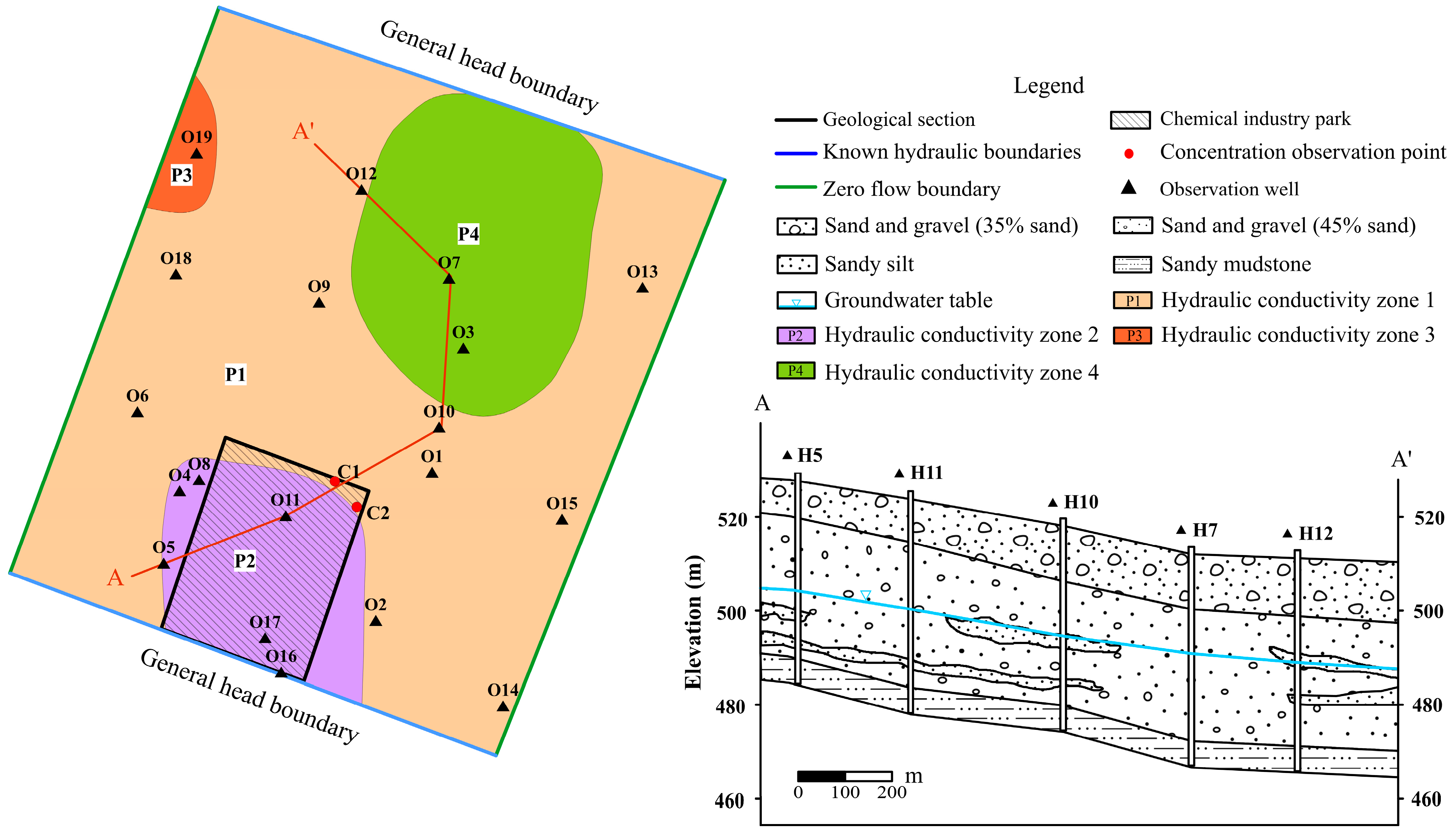
2.1. Study Area Overview

The study area was a chemical park in China. The study area was 5 million m². The maximum and minimum elevation of the area were 480 and 520 m. It has a typical continental arid climate with hot summers and cold winters, a multi-year average rainfall of 15.8 mm, and an average annual evaporation of 2293.3 mm. The recharge of rainfall to the groundwater in this area is not obvious. The groundwater is not significantly affected by evaporation because of its general depth of more than 10 m in the study area. The study area has no rivers and lakes and groundwater is not significantly exploited. The groundwater in the study area only receives recharge and discharge from lateral seepage. The interannual variation in the groundwater level is not significant, and it can be assumed that the groundwater level remains stable all year round.

Figure 1 shows the 19 water level observation points of the study area unconfined aquifer (which is the focus of this study). The groundwater flows from south to north, while the unconfined aquifer thickness also gradually increases from south to north. The lithology is a sand and pebble gravel layer, with the presence of a powder layer in some areas. The study area, guided by the different cementation degree of gravel and sand layer, is divided into 4 parameter zones. The eastern and western boundaries of the study area are perpendicular to the water table and there are zero flow boundaries. The southern and northern boundaries are known as hydraulic boundaries.

The chemical company in the study area, which produces methanol, was established in February 2013, In order to ensure the production and living water quality of downstream residential areas, it is necessary to identify the current status of pollution of regional groundwater by the chemical industry park, and to sample the water level monitoring points. The monitoring indexes were pH, salinity, metasilicic acid, total hardness, carbonate, bicarbonate, sulfate, chloride, fluoride, cyanide, nitrate, nitrite, ammonia nitrogen, permanganate index, COD, volatile phenol, iodide, arsenic, mercury, hexvalent chromium, lead, cadmium, manganese, aluminum, selenium, zinc, etc. During the August 2021 groundwater sampling run, the pollutants exceeding the water quality standard were Mn²⁺, ammonia nitrogen and volatile phenol. This paper considers only the Mn²⁺ contamination. The groundwater contamination in the chemical park was divided into three main areas (Figure 2). The leakage points in the accident pond and pretreatment area were determined via a site survey, and the contamination range of two sources was determined via groundwater monitoring at points C1-C19. The observed chemical concentrations at monitoring points Obs1 and Obs2 were significantly higher than those of points C3 and C11, indicating that there was at least one more source of pollution between these four points. However, the site investigation did not reveal any possible contamination leakage from any ground structures. It is therefore likely that the contamination occurred during the historical operation of the company, and possibly there is only one source of contamination. During the site investigation, no suspected source of pollution was found. The possibility of long-term anthropogenic discharge of pollutants was ruled out; therefore the length of the pollution leak should not be too long. The longest conservatively estimated length for pollution leakage should not exceed 1000 days. If taking the day the company began operations as day 1, it was estimated that the leak would have occurred no later than day 3150.

Table 1. Pollution source and aquifer parameters.

Parameters	Value/Range
Hydraulic conductivity (m·d−1)	0.01~15
Specific yield (%)	0.2
Longitudinal dispersivity (m)	20
Horizontal dispersivity (m)	4
Pollution source concentration (mg·L−1)	500~9000
The pollution sources leaking time (d)	1~1000

shows the aquifer and the contamination source parameters.

2.2. Bayesian Optimization Methods

Various model parameters, including black box models, were optimized via Bayesian optimization methods [32,33]. The calibration of the groundwater flow model presented in this paper required adjustment of the hydraulic conductivity in four different regions. The manual adjustment of parameters was time-consuming and challenging, so a Bayesian optimization method was chosen to perform the calibration. For the sample set consisting of n hydraulic conductivity vectors [p₁, p₂, ⋯, p_s, ⋯, p_r, where p_s denotes the s-th hydraulic conductivity vector, the Bayesian optimization process was as follows:

2.2.1. Gaussian Process Estimation

The set [L(p₁), L(p₂), ⋯, L(p_s), ⋯, L(p_r)] was obtained by selecting r samples in [p₁, p₂, ⋯, p_s, ⋯, p_r] and calculating the loss function of the calculated and observed values of the model water level corresponding to the vector of the hydraulic conductivity. A new set of observation points D_r = {(p_s, L(p_s)), s = 1, 2, …, r} could then be constructed. The D_r obeyed the Gaussian distribution as shown in the Equation (1):

$$\left\{\begin{array}{l}L(p_s)~N(0,K)\begin{array}{c}\hspace{1em}\hspace{1em}s=1,2,\cdots \end{array},r\\ K=\left[\begin{array}{l}k(p_1,p_1)\cdots k(p_1,p_r)\\ \begin{array}{c}\begin{array}{c}⋮\end{array}\end{array}⋮\\ k(p_r,p_1)\cdots k(p_r,p_r)\end{array}\right]\end{array}\right.$$

(1)

where: k(p_r, p_r) is the kernel function, representing the covariance and K is the covariance matrix.

2.2.2. Adding New Observation Points

Additional observation points had to be added at suitable locations to estimate the distribution of the objective function more accurately. The PI method (Probability of Improvement) and the EI method (Expected Improvement) are commonly used to search observation points [34,35]. We used the EI method to identify additional observation points as it has a wider search domain. New sampling points were determined via the EI method by comparing the mathematical expectation of the loss function of the current sampling point and other sampling points. Assuming that p⁺ is the optimal hydraulic conductivity vector inside the existing observation points, and y* is the threshold value larger than L(p⁺), the mathematical expectation E(p_s) can be expressed by Equation (2):

$$\left\{\begin{array}{l}E(p_s)={\displaystyle {\int }_{-\infty }^{y^{*}}(y^{*}-y)P(y|p_s)}dy=\frac{\mathcal{l}(p_s)(\gamma y^{*}-{\displaystyle {\int }_{-\infty }^{y^{*}}P(p_s)}dy)}{\gamma \mathcal{l}(p_s)+(1-\gamma )g(p_s)}\\ P(p_s|y)=\left\{\begin{array}{l}\mathcal{l}(p_s)\hspace{1em}\hspace{1em}\hspace{1em}y\le y^{*}\\ g(p_s)\hspace{1em}\hspace{1em}\hspace{1em}y>y^{*}\end{array}\right.\end{array}\right.$$

(2)

where: P(y|p_s) is the probability density function; γ is the distribution weight; $\mathcal{l}$(p_s) is the distribution function when $y\le y^{*}$; and g(p_s) is the distribution function when $y>y^{*}$. The vector of the hydraulic conductivity p_best that gives the optimal mathematical solution as shown in Equation (3), was selected as the new sampling point.

$$p_{best}=\arg \max E(p_s)$$

(3)

where: $\arg \max E(p_s)$ represents the p_s that provides the optimal E(p_s). These newly selected sampling points allow for a more accurate estimate of the distribution of the loss function.

2.2.3. Update the Gaussian Distribution of L(p_s)

The new Gaussian distribution as shown in Equation (4) could be determined after adding the new observation points.

$$\left\{\begin{array}{l}\left[\begin{array}{l}\left[L(p_1),L(p_2),\cdots ,L(p_r)\right]\\ L(p_{best})\end{array}\right]~N\left(0,\left[\begin{array}{cc}K\hfill & k^{\prime }\\ {(k^{\prime })}^{\mathrm{T}}\hfill & k(p_{best},p_{best})\end{array}\right]\right)\\ k^{\prime }=[k(p_{best},p_1),k(p_{best},p_2),\cdots ,k(p_{best},p_r)]\end{array}\right.$$

(4)

The new distribution P(F(p_best)|D_r, p_best) of L(p_r + 1) can then be calculated by Equation (5):

$$\left\{\begin{array}{l}p(L(p_{best}|D_r,p_{best}))~N(\mu ,{\sigma }^2)\\ \mu ={(k^{\prime })}^{\mathrm{T}}{K}^{-1}[L(p_1),L(p_2),\cdots ,L(p_r)]\\ {\sigma }^2=k(p_{best},p_{best})-{(k^{\prime })}^{\mathrm{T}}{K}^{-1}{k}^{\prime }\end{array}\right.$$

(5)

where: μ, and σ are the mean and standard deviation, respectively.

The model estimates the loss function more accurately over time by continuously looping ② and ③. This means that there is an increasing probability of accurately estimating the extreme values of the loss function and the corresponding optimal parameters. Bayesian optimization stops after the loop reaches the maximum number of iterations, after which the optimal point is provided as output.

The certainty coefficient (R²) between the calculated water level and the actual water level at the water level observation point in this model was used to determine the goodness of the model fit. The closer the R² is to 1, the better the calculated water level fits the actual water level and the more accurate the predicted hydraulic conductivity value. The loss function of the Bayesian optimization model above is R² and the optimization objective is to find a combination of hydraulic conductivity that maximizes R². R² can be calculated by using Equation (6):

$$R^2=1-\frac{{{\displaystyle \sum \left(y_i-{\widehat{y}}_i\right)}}^2}{{{\displaystyle \sum \left(y_i-\overline{y}\right)}}^2}$$

(6)

where: ${\widehat{y}}_i$ is the calculated value of the water level at the i-th observation point; y_i is the measured value of the water level at the i-th observation point; and $\overline{y}$ is the average value of all measured water levels.

2.3. SEGA Algorithm

The SEGA algorithm is a genetic algorithm that uses the elite retention strategy [36]. This genetic algorithm is similar to the biological evolutionary process, where only the fittest chromosomes are retained [37]. In a genetic algorithm, the competition between individual chromosomes is achieved by calculating the fitness of each chromosome. Chromosomes with high fitness have a higher probability of surviving and passing their genes on to the next generation, while those with low fitness have a higher probability of being eliminated. Several natural selection strategies can be used, including roulette and tournaments [38]. The tournament method has the advantage of not easily falling into local optimal solutions, is not very complex, and allows for parallelization processing. It is therefore the most popular selection strategy in genetic algorithms. Algorithm 1 shows the basic process of the SEGA algorithm. The algorithm starts by selecting a random part of the solutions from the solution space of the problem as the initial population. It considers each solution in the population as a chromosome, which is a sequence of numbers or a sequence of strings constructed by special coding rules [39]. Each element in the sequence is a gene that constitutes the chromosome.

Algorithm 1: Strengthen Elitist GA Algorithm

Begin SEGA

Initialize the population according to the code rules

Retain the best population

do

Evaluate fitness value and optimal individuals

Perform Selection

Perform Crossover on candidates with a high fitness value

Perform Mutation on candidates with a high fitness value

Update the best population with optimal individuals

while (termination threshold is not met)

return the best population

End SEGA

All the chromosomes in the population are allowed to evolve towards a given goal (the optimal solution) and to compete for survival during the evolutionary process. The laws of nature will come into play at this point where the winners in this competition will be retained, while the losers will be eliminated.

All the winners, except for the optimal chromosome, will produce many new individuals to replace the eliminated losers by crossover and mutation (Figure 3). The total population will therefore be kept intact while allowing the best genes to be passed on, which is called elite retention [40,41]. The elite retention method uses a reduced number of iterations to avoid a prolonged convergence time of the algorithm, which is caused by avoiding the destruction of good genes by crossover and mutation. Increasing the genetic diversity of the pool by a gene mutation is more likely to generate new optimal chromosomes and is less likely to cause the algorithm to fall into local optimal solutions. The elite retention method that is used by the SEGA algorithm may, however, cause the algorithm to fall into a local optimal solution after only a few iterations. This problem is avoided by setting larger crossover and mutation probabilities in the SEGA algorithm.

After each round of chromosome competition for survival, genetic recombination, and mutation, the new chromosome population, containing the best genes, constitutes the “next generation”. This generation will continue to evolve toward the final goal of survival and compete again. Each generation is the offspring of the winner, therefore the new generation will be stronger than the previous one, and the population will gradually advance toward the set goal.

2.4. Coupling of Simulation-Optimization Models

We used Python application libraries such as FloPy, Geatpy, and Bayes_opt to construct a simulation-optimization model for solving the practical problem of groundwater contaminant traceability in this paper. The Bayesian optimization was used to calibrate the water flow model and the SEGA algorithm was used to find the contaminant source location and model parameters related to the release history. Figure 4 shows the structure of the whole model.

The model structure is combined with several different parts (Figure 4). The simulation-optimization model includes two parts: simulation and optimization. The simulation part includes both numerical simulations of groundwater flow and solute transport simulation, while the optimization part generally only optimizes the solute transport model. However, for this paper, the optimization of parameters for the groundwater flow was added. The model coupling can be divided into two categories: firstly the coupling of the FloPy-based code and the numerical calculation software, which is the coupling of two technologies; secondly, the coupling of numerical seepage and solute transport models with the optimization algorithms, which is the intersection of two theories.

Compared to other Python application libraries, the numerical models coded by FloPy are not computed by underlying scripts based on the Python language. Instead, the models are compiled into input files corresponding to simulation software such as MODFLOW and MT3DMS. The computation process was performed by this software and allows the user to upload the results from the files generated by the numerical simulation software onto FloPy. FloPy designs the models while the numerical simulation software solves the models.

The implementation of the first coupling described above, provides the conditions for the second coupling. Only the inputs and outputs in the optimization problem are important for the optimization algorithms such as Bayesian optimization and evolutionary algorithms, and not the computational process of the results. Therefore, the seepage model and the solute transport model can be coded into two functions. Here, the inputs are the parameters to be optimized in the corresponding models and the outputs are the results of the model runs, respectively. In this way, the groundwater model can be transformed into a generalized objective function to be optimized, providing an appropriate optimization method to find the optimal solution.

3. Model Details

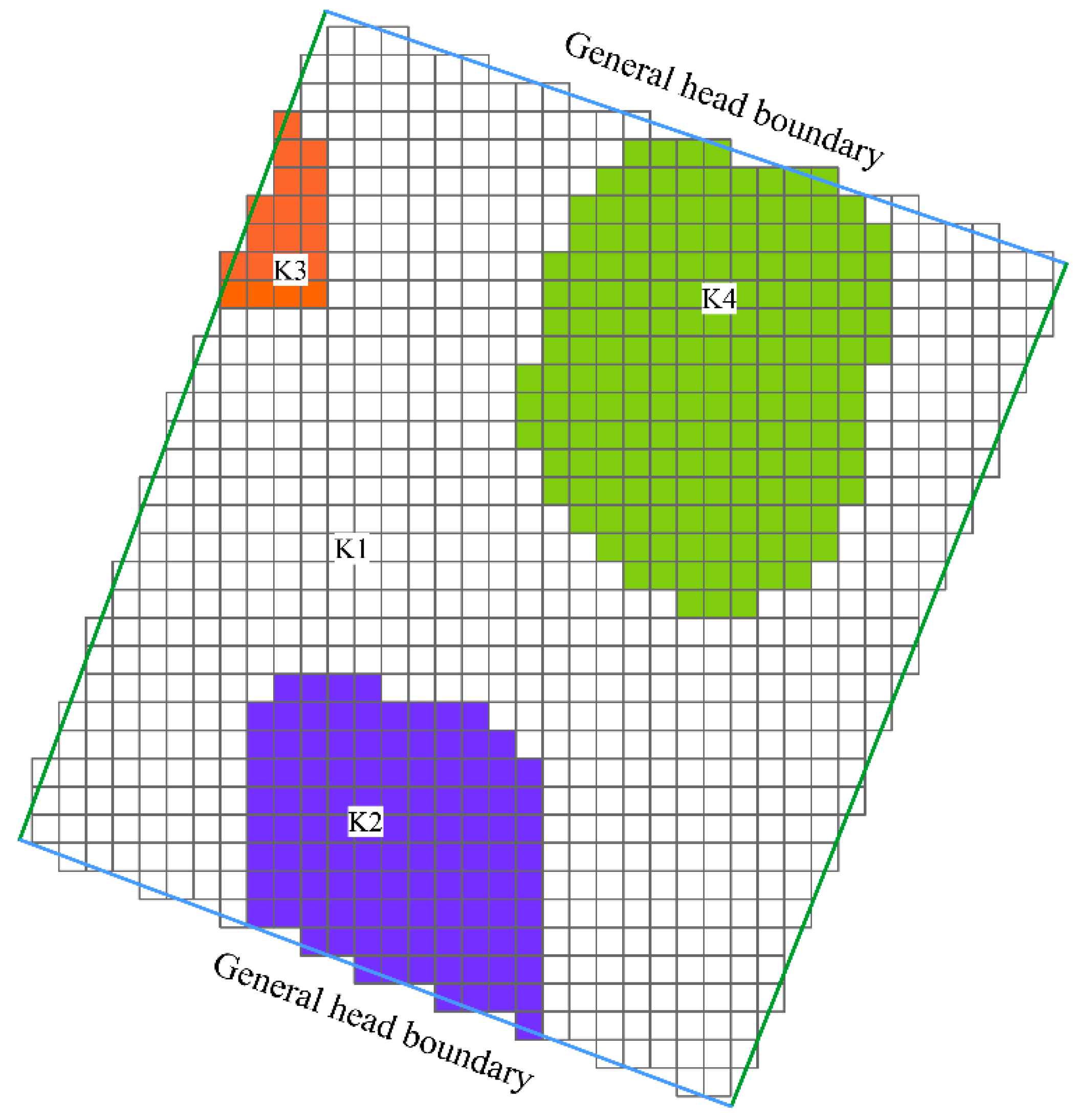
3.1. Groundwater Flow Model Parameter Optimization and Calibration

A preliminary water flow model can be built using Visual Modflow or GMS to speed up the model building and reduce the number of codes. The resultant model can then be loaded using FloPy and coupled with Bayesian optimization methods for parameter optimization. In the preliminary establishment of a flow model, the initial conditions and boundary conditions need to be described in the model. In this study, the initial conditions were the initial water head distribution in the study area; the east-west boundary was described as the confining boundary, and the north-south boundary was described as the general head boundary. The study area was generalized as a heterogeneous isotropic aquifer (1950 m × 2330 m) and was discretized into a grid consisting of 911 rectangles of 75.7 m × 72.2 m (Figure 5). The hydraulic conductivity of the study area was divided into four zones: K₁, K₂, K₃, and K₄, based on the lithology and the measured groundwater flow field. The northern and southern boundaries were set as general head boundaries (GHBs).

The core code lines and coding logic are shown below:

1) mod = flopy.modflow.Modflow.load(Vmod.nam)

2) lpf = flopy.modflow.ModflowLpf(model = mod, hk = New_K)

3) mod.write_input()

The first line of code was used to load the water flow model and requires the input of the model’s NAM file. In some Python environments, relative paths need to be used in the NAM file to load the model correctly. The NAM file used in this model is in the same format as the input of MODFLOW.

The second line of code overwrites the LPF file to change the hydraulic conductivity of the model while the optimization program is running. This method requires passing in the loaded model mod and the new hydraulic conductivity matrix New_K. The hydraulic conductivity of the model can be overwritten if the groundwater flow model is built with the block-centered flow package (BCF), using the following code:

4) bcf = FloPy.modflow.ModflowBcf(model = mod, hy = New_K)

With the third line of code, FloPy recompiles the loaded model into MODFLOW format input files.

Bayesian optimization using Python is now simply a matter of passing in the objective function and a priori information about the hydraulic conductivity in the code (see line 5). In this paper, Bayesian Optimization was used to build the optimization model. The initial sampling points for Bayesian optimization were set to 4, and the cycle was 1000 times. The hydraulic conductivity at the observation points within each zone determined the prior information of the hydraulic conductivity zone.

5) bs_pto = BayesianOptimization(

       obj_function,

       {‘k1’: (0.5, 2), ‘k2’: (1, 5), ‘k3’: (0.01, 1), ‘k4’: (5, 15)})

The objective function of Bayesian optimization can be a generalized objective function, which only considers the input and output of the function. Json can be used to save the parameters after each run The hydraulic conductivity is the input of the function, and the determinant coefficients (R2) of the observed and measured head values are the output of the function. The closer the R2 value is to 1, the more accurate the predicted hydraulic conductivity value. The programming logic of the target function is shown below:

6) def obj_function(K₁, K₂, K₃, K₄):

    Load flow model

    Change the hydraulic conductivity

    Run the model

    Read the calculated head value

    Calculate R²

    return R²

By following the above steps, the hydraulic conductivity of the groundwater flow model can be easily optimized using the Bayesian optimization method. If you want to optimize other parameters, you only need to change the optimized parameters in the above model.

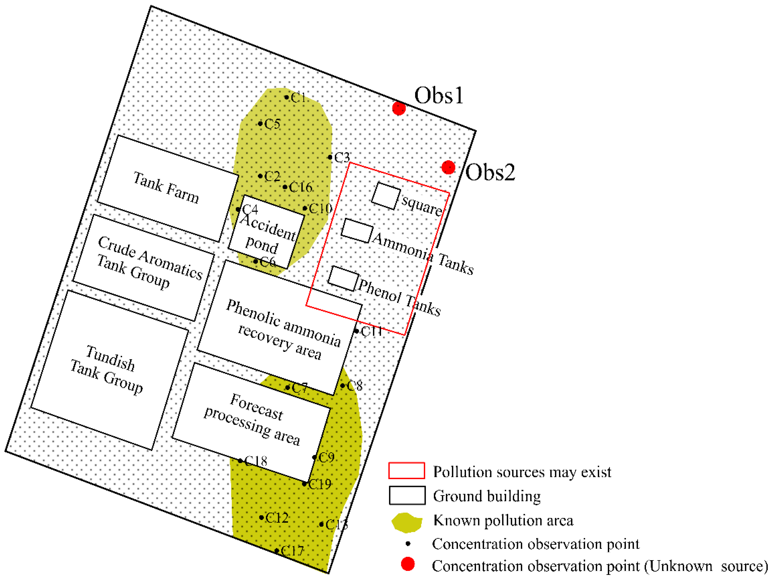
3.2. Simulation-Optimization Model for Pollutant Traceability

The simulation-optimization model consists of two parts: simulation and optimization. The optimization part of the model is composed of three parts: (1) minimization of the mean square error between the observed and simulated values of the pollution concentrations for each observation well as an objective function; (2) the parameters that determine the release history of the groundwater contaminants as the decision variables; and (3) the decision variables that satisfy the groundwater solute transport law and a reasonable geographical range as the constraints. The simulation part is equivalent to the generalized objective function in the optimization part. The decision variables in the optimization part are the parameters controlling the release of pollution sources in the simulation part. The mathematical expression of the optimization part is shown in Equation (7):

$$\begin{array}{l}Objectivefunction:\\ \min f\left(x_n\right)=\mathrm{MSE}\left(C_{calc}\left(x_n\right),C_{obs}\right)\\ Constraints:\\ \left\{\begin{array}{l}15<x_1<20\\ 28<x_2<33\\ 500<x_3<9000\\ 2000<x_4<3000\\ 0<x_5<1000\\ x_4+x_5<3150\end{array}\right.\end{array}$$

(7)

Here, C_calc is the value of the concentration observation point calculated by the model; C_obs is the observed value of the measured concentration. x₁ is the column where the source is located; x₂ is the row where the source is located; x₃ is the release concentration of the source; x₄ is the time when the source starts to release; and x₅ is the duration of the leak of the source. All the decision variables are integers. The SEGA algorithm solved the above single-objective optimization problem (with the algorithm parameters shown in

Table 2. SEGA parameters.

Parameters	Value
Encoding	Real integer encoding (RI)
Number of individuals	30
Maximum number of generations	100
trappedValue	0.000001
maxTrappedCount	10

). Here, the trappedValue represents the judgment threshold of evolutionary stagnation (the local optimal solution); and maxTrappedCount represents the maximum number of times evolution is allowed to stagnate.

The above optimization model is coded and solved using Geatpy2 [42]. Using Geatpy2, the evolutionary algorithm framework can be built quickly and concisely. The key code defining the generalized objective function is shown below. To construct the objective function, a solute transport model based on the water flow model coded in the previous section, using FloPy, is needed. The following code can be used to modify the time discretization of the water flow model and to add injection wells for releasing the contaminant sources.

7) dis = flopy.modflow.ModflowDis(model = mod, nper = nper, steady = steady, perlen = perlen)

8) wel = flopy.modflow.ModflowWel(model = mod, stress_period_data = spd)

9) lmt = flopy.modflow.ModflowLmt(model = mod, output_file_name = ‘mt3d_link.ftl’)

Line 7 of the code can modify the model time discretization parameters, where nper represents the number of stress periods (which is set to 4 in this paper); steady is a list indicating the flow state of each stress period (which can only contain True or False, where True means that the corresponding stress period is stable flow, and False indicates that the flow state is unstable); and perlen is a list of all the stress period lengths.

Line 8 of the code can add injection wells, where stress_period_data is a dictionary containing well locations, injection rates, and stress periods.

Line 9 of the code is used to create the FTL file linking MODFLOW and MT3DMS. The following code is used to create the solute transport model and compile the MT3DMS input file:

10).mt = flopy.mt3d.Mt3dms(modelname = ‘mt’, exe_name = ‘mt3dms5b’, modflowmodel = mod)

11) btn = flopy.mt3d.Mt3dBtn(mt, munit = ‘mg/L’, obs = obs, nprs = nprs, timprs = timprs)

12) adv = flopy.mt3d.Mt3dAdv(mt, mixelm = −1, percel = 1)

13) dsp = flopy.mt3d.Mt3dDsp(mt, al = 20, trpt = 0.2)

14) ssm = flopy.mt3d.Mt3dSsm(mt, stress_period_data = spd_mt)

15) gcg = flopy.mt3d.Mt3dGcg(mt, mxiter = 1000, iter1 = 200, isolve = 1, cclose = 0.0001)

16) mt.write_input()

17) mt.run_model(silent = True)

Line 10 of the code initializes the MT3DMS model.

Line 11 of the code sets the MT3DMS basic transmission package parameters, where obs is a list containing the locations of concentration observation points, nprs is the number of concentration observations, and timprs is a list of observation times corresponding to the number of observations. nprs and timprs mainly reflect the preservation of the concentration values at each point at different moments in time.

Line 12 of the code sets the parameters for the selection of the advection calculation scheme. Here, mixelm is an integer flag for the advection solution option. When the value is −1, it means that the third-order TVD scheme is used. For the third-order TVD scheme, percel is a stability constraint that must not exceed one and will be automatically reset to one if a value greater than one is specified.

In line 13 of the code, the al is the longitudinal dispersivity. For every cell of the model grid; the trpt is a real array defining the ratio of the horizontal transverse dispersivity to the longitudinal dispersivity.

The stress_period_data in line 14 of the code is a dictionary containing the location, concentration, and stress period of the pollution source.

Line 15 of the code is used to set the relevant parameters in the gcg solution method. mxiter is the maximum number of outer iterations; iter1 is the maximum number of inner iterations; and isolve is the type of preconditioners to be used with other acceleration schemes. When the value is 1, the Jacobi scheme is used.

Lines 16 and 17 of the code compile and run the solute transport model.

The calculated concentrations can be loaded from the model results once the entire groundwater model is completed. This provides the value of the parameter C_calc in the objective function in Equation (7), which allows for the calculation of the objective function values for the optimization problem. This procedure allows for the groundwater pollution traceability problem to be transformed into an optimization problem, which can be solved using the SEGA algorithm.

4. Results and Discussions

4.1. Groundwater Flow Model Optimization Results

Table 3. Bayesian optimization results.

Parameters	Value
R2	0.979
K1	0.727
K2	2.510
K3	0.550
K4	11.590

shows the optimal Bayesian parameter optimization results. The best determination hydraulic conductivity value was as high as 0.979, indicating that the model achieved a good optimization result. The optimal value of the hydraulic conductivity zoning obtained from the Bayesian parameter optimization result was brought into the groundwater numerical model, which can simulate the calculated water level of the model in the study area. The accuracy of the constructed numerical model can be verified by comparing the calculated water level of the model with the actual observed water level. The slope of the fitted curve between the model-calculated water level and the actual observed water level is 0.914 (Figure 6), which is very close to the best-fit line y = x. All the model points lie within the 95% prediction interval, indicating that the simulated groundwater flow field is reliable enough to be used to model contaminant transport. Bayesian parameter optimization results were used to simulate the local groundwater flow field. The groundwater, guided by the hydraulic gradient, flows from south to north (Figure 7).

4.2. Simulation-Optimization Model Results

Table 4. Inversion results of the pollution sources.

Parameters	Value
x1	19
x2	28
x3 (mg·L−1)	6631
x4 (d)	2000
x5/(d)	354
Evaluation number	1350
Execution time (s)	411
Best objective value	0.35
Total number of generations	45

shows the simulation-optimization model results. Our SEGA model evolved for 45 generations and evaluated a total of 1350 chromosomes to obtain the optimal objective function value of 0.35. The pollution source is located in the 19th column and 28th rows of the model. The pollution source leaked at a concentration of 6631 mg/L⁻¹ Mn²⁺ on the 2000th day after the chemical plant was put into operation, leaking for 354 days. Figure 8 shows the convergence of the optimal objective function while solving for the pollution source. The model found a good solution after 19 iterations and then entered a smoother convergence process until it converged (Figure 8). The model runs in 411 s, which is an acceptable amount of time spent.

Figure 9 shows the fit of the pollutant concentrations at the two observation points. The blue and green curves in the figure are the calculated pollutant concentrations at Obs1 and Obs2, respectively, and the red points are the actual observed concentration values. Figure 9 shows that the simulated pollutant concentrations match the observed pollutant concentrations well.

Figure 10 shows the location and extent of the contamination source as obtained by the simulation-optimization model. The pollution source is located inside the square. The initial site investigations did not indicate any trace of pollution leakage and no industrial equipment was present where leakage may have occurred inside the square. The site investigation results, therefore, contradict the simulation results. A subsequent site visit to the people around the square brought to light that the square was used to dry sludge in the biochemical pond about two years ago. This sludge contains a large amount of sewage, which seeped into the ground during drying, causing groundwater contamination. This history of the site contamination investigated agrees with the traceability results. Therefore, the source locations obtained from the simulation-optimization model are verified to be reliable. However, the leak times and concentrations of the sources cannot be accurately verified. The purpose of exploring the pollution source location and release history at this site was to stop the pollution in time and to develop subsequent treatment plans. The simulated pollutant transport history is consistent with the actual observation, making the simulation results of the simulation-optimization model reliable. This study, therefore, achieved its research purpose.

5. Conclusions

In order to realize the traceability of single-target pollutant sources in chemical parks, this paper utilizes FloPy to tightly couple multiple algorithms and models, which are originally complex, with a small amount of code. A tightly coupled three-dimensional numerical model of groundwater solute transport was formed of the groundwater flow model constructed by Bayesian optimization algorithm and the solute transport model constructed by the SEGA algorithm. The pollutant traceability problem was successfully solved in this study. The main conclusions of this paper are as follows:

(1)

FloPy makes it easy to build a groundwater flow model with code, while Bayesian optimization achieves better results than the manual optimization of parameters, with an R² of 0.979. The code framework that was developed can be applied to different models with only a few parameter changes.

(2)

The SEGA algorithm was used to solve the groundwater pollution traceability problem by transforming it into a single-objective optimization problem with good results. This method can be easily applied to practical work because of its small amount of code, simple structure, and short time consumption.

(3)

The Python-based FloPy library greatly reduces the difficulty of automatic inversion of groundwater pollution traceability. This will effectively promote the application of complex theoretical methods to practical problems. It allows for traditional numerical models to be more simply and effectively combined with new numerical techniques, thereby breaking through the limitations of traditional commercial software and further promoting the development of the numerical groundwater simulation field.

(4)

Based on FloPy and Bayesian optimization algorithms, the SEGA algorithm can construct a tightly coupled groundwater solute transport model in the chemical park, aiming at the location of the pollution source to find the source of heavy metal manganese leakage from the perspective of preventing industrial wastewater leakage and protecting groundwater. Compared with the traditional water chemistry characterization method and isotope technology, the application is efficient and flexible, and the calculation can reason the pollution situation in the forward direction, which can make a more accurate judgment on the source of pollutants.

Many improvements can be made to this paper, such as using only one optimization method to solve the hydraulic conductivity and the pollution source at the same time, in order to further reduce the complexity of the model; in the face of the superposition of multiple sources of pollution, it is possible to further combine FloPy and the multi-objective optimization genetic algorithm to build a multi-objective groundwater simulation optimization model with the location of the source of pollution as the goal.

References

1. Konikow, L.F. Role of numerical simulation in analysis of ground-water quality problems. Sci. Total Environ. 1981, 21, 299–312. [Google Scholar] [CrossRef]
2. Langevin, C.D.; Panday, S. Future of Groundwater Modeling. Groundwater 2012, 50, 333–339. [Google Scholar] [CrossRef]
3. McDonald, M.G.; Harbaugh, A.W.; Geological Survey (U.S.). A modular Three-Dimensional Finite-Difference Ground-Water Flow Model; Scientific Publications Co. Distributor: Washington, DC, USA, 1984; p. vi. 528p.
4. Sundar, M.L.; Ragunath, S.; Hemalatha, J.; Vivek, S.; Mohanraj, M.; Sampathkumar, V.; Ansari, A.M.S.; Parthiban, V.; Manoj, S. Simulation of ground water quality for noyyal river basin of Coimbatore city, Tamilnadu using MODFLOW. Chemosphere 2022, 306, 135649. [Google Scholar] [CrossRef]
5. Bo, Q.Y.; Cheng, W.Q.; Sun, T. Groundwater Simulation Model for Baohe River in the Upper Reaches of Baiyangdian Lake Based on Groundwater Simulation Software (Gms). J. Environ. Prot. Ecol. 2021, 22, 1162–1174. [Google Scholar]
6. Yang, Y.; Zhu, Y.; Wu, J.W.; Mao, W.; Ye, M.; Yang, J.Z. Development and application of a new package for MODFLOW-LGR-MT3D for simulating regional groundwater and salt dynamics with subsurface drainage systems. Agric. Water Manag. 2022, 260, 107330. [Google Scholar] [CrossRef]
7. Morway, E.D.; Langevin, C.D.; Hughes, J.D. Use of the MODFLOW 6 Water Mover Package to Represent Natural and Managed Hydrologic Connections. Groundwater 2021, 59, 913–924. [Google Scholar] [CrossRef] [PubMed]
8. Pietrzak, D. Modeling migration of organic pollutants in groundwater—Review of available software. Environ. Model. Softw. 2021, 144, 105145. [Google Scholar] [CrossRef]
9. Xu, Z.P.; Zhou, X.; Chen, R.G.; Shen, Y.; Shang, Z.Q.; Hai, K. Numerical Simulation of Deep Thermal Groundwater Exploitation in the Beijing Plain Area. Water 2019, 11, 1494. [Google Scholar] [CrossRef]
10. Banaei, S.M.A.; Javid, A.H.; Hassani, A.H. Numerical simulation of groundwater contaminant transport in porous media. Int. J. Environ. Sci. Technol. 2021, 18, 151–162. [Google Scholar] [CrossRef]
11. Seyf-Laye, A.-S.M.; Mingzhu, L.; Djanéyé-Bouindjou, G.; Fei, L.; Lyutsiya, K.; Moctar, B.L.; Honghan, C. Groundwater flow and contaminant transport modeling applications in urban area: Scopes and limitations. Environ. Sci. Pollut. Res. 2012, 19, 1981–1993. [Google Scholar] [CrossRef]
12. Ben Simon, R.; Bernard, S.; Meurville, C.; Rebour, V. Flow-Through Stream Modeling with MODFLOW and MT3D: Certainties and Limitations. Groundwater 2015, 53, 967–971. [Google Scholar] [CrossRef] [PubMed]
13. Kumar, C. An overview of commonly used groundwater modelling software. Int. J. Adv. Sci. Eng. Technol. 2019, 6, 7854–7865. [Google Scholar]
14. Tabari, M.M.R.; Eilbeigi, M.; Chitsazan, M. Multi-objective optimal model for sustainable management of groundwater resources in an arid and semiarid area using a coupled optimization-simulation modeling. Environ. Sci. Pollut. Res. 2022, 29, 22179–22202. [Google Scholar] [CrossRef] [PubMed]
15. Matott, L.S.; Leung, K.; Sim, J. Application of MATLAB and Python optimizers to two case studies involving groundwater flow and contaminant transport modeling. Comput. Geosci. 2011, 37, 1894–1899. [Google Scholar] [CrossRef]
16. Bakker, M.; Post, V.; Langevin, C.D.; Hughes, J.D.; White, J.T.; Starn, J.J.; Fienen, M.N. Scripting MODFLOW Model Development Using Python and FloPy. Groundwater 2016, 54, 733–739. [Google Scholar] [CrossRef]
17. Rahmati, O.; Moghaddam, D.D.; Moosavi, V.; Kalantari, Z.; Samadi, M.; Lee, S.; Tien Bui, D. An automated python language-based tool for creating absence samples in groundwater potential mapping. Remote Sens. 2019, 11, 1375. [Google Scholar] [CrossRef]
18. Bakker, M.; Post, V.; Hughes, J.; Langevin, C.; Francés, A.P.; White, J. Enhanced FloPy scripts for constructing and running MODFLOW-based models. In Proceedings of the MODFLOW and More 2013: Translating Science and Practice, Golden, CO, USA, 2–5 June 2013. [Google Scholar]
19. Foglia, L.; Borsi, I.; Mehl, S.; De Filippis, G.; Cannata, M.; Vasquez-Sune, E.; Criollo, R.; Rossetto, R. FREEWAT, a free and open source, GIS-integrated, hydrological modeling platform. Groundwater 2018, 56, 521–523. [Google Scholar] [CrossRef]
20. De Smet, S. The Effect of Brackish Water Extraction on the Brackish Upconing Below the Horstermeer Polder: Creating a 3D Regional Variable-Density Groundwater Model using MODFLOW 6 and FloPy. Master’s Thesis, Delft University of Technology, Delft, The Netherlands, 2021. [Google Scholar]
21. J-Y, J.; YN, J. Groundwater Simulation Optimization Model Based on FloPy and NSGA-III. Water Resour. Power 2021, 39, 2. [Google Scholar]
22. Wei, Y.; Chen, J.; Zhang, D.; Li, L. Application and Research Progress of Python in Groundwater Numerical Simulation. Comput. Technol. Dev. 2021, 31, 150–156. (In Chinese) [Google Scholar]
23. Li, B.; Lu, Y.; Li, J.; Jiang, H.; Wang, Y. Exploring the spatial-temporal variations and policy-based driving force behind groundwater contamination and remediation research in past decades. Environ. Sci. Pollut. Res. 2021, 28, 13188–13201. [Google Scholar] [CrossRef]
24. Milnes, E.; Perrochet, P. Simultaneous identification of a single pollution point-source location and contamination time under known flow field conditions. Adv. Water Resour. 2007, 30, 2439–2446. [Google Scholar] [CrossRef]
25. Wang, X.; Xu, Y.J.; Zhang, L. Watershed scale spatiotemporal nitrogen transport and source tracing using dual isotopes among surface water, sediments and groundwater in the Yiluo River Watershed, Middle of China. Sci. Total Environ. 2022, 833, 155180. [Google Scholar] [CrossRef]
26. Li, J.; Wu, Z.; He, H.; Lu, W. Comparative analysis of groundwater contaminant sources identification based on simulation optimization and ensemble Kalman filter. Environ. Sci. Pollut. Res. 2022, 29, 90081–90097. [Google Scholar] [CrossRef] [PubMed]
27. Yao, L.; Guo, Y. Hybrid algorithm for parameter estimation of the groundwater flow model with an improved genetic algorithm and gauss-newton method. J. Hydrol. Eng. 2014, 19, 482–494. [Google Scholar] [CrossRef]
28. Huang, L.; Wang, L.; Zhang, Y.; Xing, L.; Hao, Q.; Xiao, Y.; Yang, L.; Zhu, H. Identification of groundwater pollution sources by a SCE-UA algorithm-based simulation/optimization model. Water 2018, 10, 193. [Google Scholar] [CrossRef]
29. Chakraborty, A.; Prakash, O. Identification of clandestine groundwater pollution sources using heuristics optimization algorithms: A comparison between simulated annealing and particle swarm optimization. Environ. Monit. Assess. 2020, 192, 791. [Google Scholar] [CrossRef]
30. Wu, M.; Wang, L.; Xu, J.; Wang, Z.; Hu, P.; Tang, H. Multiobjective ensemble surrogate-based optimization algorithm for groundwater optimization designs. J. Hydrol. 2022, 612, 128159. [Google Scholar] [CrossRef]
31. Kontos, Y.N.; Kassandros, T.; Perifanos, K.; Karampasis, M.; Katsifarakis, K.L.; Karatzas, K. Machine learning for groundwater pollution source identification and monitoring network optimization. Neural Comput. Appl. 2022, 34, 19515–19545. [Google Scholar] [CrossRef]
32. Greenhill, S.; Rana, S.; Gupta, S.; Vellanki, P.; Venkatesh, S. Bayesian optimization for adaptive experimental design: A review. IEEE Access 2020, 8, 13937–13948. [Google Scholar] [CrossRef]
33. Pan, Z.; Lu, W.; Fan, Y.; Li, J. Identification of groundwater contamination sources and hydraulic parameters based on bayesian regularization deep neural network. Environ. Sci. Pollut. Res. 2021, 28, 16867–16879. [Google Scholar] [CrossRef]
34. Jones, D.R. A taxonomy of global optimization methods based on response surfaces. J. Glob. Optim. 2001, 21, 345–383. [Google Scholar] [CrossRef]
35. Chaudhuri, A.; Haftka, R.T. Efficient global optimization with adaptive target setting. AIAA J. 2014, 52, 1573–1578. [Google Scholar] [CrossRef]
36. Jayaram, M.; Nataraja, M.; Ravikumar, C. Elitist genetic algorithm models: Optimization of high performance concrete mixes. Mater. Manuf. Process. 2009, 24, 225–229. [Google Scholar] [CrossRef]
37. Michalewicz, Z.; Schoenauer, M. Evolutionary algorithms for constrained parameter optimization problems. Evol. Comput. 1996, 4, 1–32. [Google Scholar] [CrossRef]
38. Katoch, S.; Chauhan, S.S.; Kumar, V. A review on genetic algorithm: Past, present, and future. Multimed. Tools Appl. 2021, 80, 8091–8126. [Google Scholar] [CrossRef]
39. Sivanandam, S.; Deepa, S. Genetic algorithms. In Introduction to Genetic Algorithms; Springer: Berlin/Heidelberg, Germany, 2008; pp. 15–37. [Google Scholar]
40. Saini, N. Review of selection methods in genetic algorithms. Int. J. Eng. Comput. Sci. 2017, 6, 22261–22263. [Google Scholar]
41. Jebari, K.; Madiafi, M. Selection methods for genetic algorithms. Int. J. Emerg. Sci. 2013, 3, 333–344. [Google Scholar]
42. Jazzbin. Geatpy: The Genetic and Evolutionary Algorithm Toolbox with High Performance in Python. Available online: http://www.geatpy.com/ (accessed on 9 January 2022).
Figure 1. Overview of the study area.
Applsci 13 10707 g001
Figure 2. Overview of the chemical industry park.
Applsci 13 10707 g002
Figure 3. Example of crossover and mutation.
Applsci 13 10707 g003
Figure 4. Model structure diagram.
Applsci 13 10707 g004
Figure 5. Model grid diagram.
Applsci 13 10707 g005
Figure 6. Comparison diagram of the Calculated Head against the Observed Head.
Applsci 13 10707 g006
Figure 7. Simulated flow field.
Applsci 13 10707 g007
Figure 8. Best objective value trace plot.
Applsci 13 10707 g008
Figure 9. Observation point concentration changes over time.
Applsci 13 10707 g009
Figure 10. Pollution traceability map.
Applsci 13 10707 g010