Microbial Colony Detection Based on Deep Learning

Abstract

In clinical drug sensitivity experiments, it is necessary to plate culture pathogenic bacteria and pick suitable colonies for bacterial solution preparation, which is a process that is currently carried out completely by hand. Moreover, the problems of plate contamination, a long culture period, and large image annotation in colony plate image acquisition can lead to a small amount of usable data. To address the issues mentioned above, we adopt a deep learning approach and conduct experiments on the AGAR dataset. We propose to use style transfer to extend the trainable dataset and successfully obtain 4k microbial colony images using this method. In addition, we introduce the Swin Transformer as a feature extraction network in the Cascade Mask R-CNN model architecture to better extract the feature information of the images. After our experimental comparison, the model achieves a mean Average Precision (mAP) of 61.4% at the Intersection over Union (IoU) [0.50:0.95]. This performance surpasses that of the Cascade R-CNN with HRNet, which is the top-performing model in experiments conducted on the AGAR dataset, by a margin of 2.2%. Furthermore, we perform experiments using YOLOv8x on the AGAR dataset, which results in a mAP of 76.7%.

1. Introduction

In clinical microbiology laboratories, we often extract secretions or blood from patients and perform bacterial cultures. The treatment is based on the results of the drug sensitivity tests [1] of the isolated pathogenic organisms. In this process, we usually use strains collected from different patients, isolate and culture them in agar or other plates, and then manually morphologically identify the colonies after they are formed and select independent, uncontaminated colonies to configure samples at appropriate concentrations for drug sensitivity tests. However, the entire process of sample collection, incubation, and final plate evaluation, including microbial colony identification, requires the full participation of the laboratory staff. The manual identification of colony types in plates [2] requires not only the experience of the laboratory personnel, but also a lot of time. Therefore, we hope to solve this problem of microbial plate identification with the help of the latest Artificial Intelligence (AI) technology.

In the last few years, picture recognition has benefited greatly from data-based AI training techniques. Since the advent of AlexNet [3], Convolutional Neural Networks (CNNs) [4,5,6] have been the standard architecture for Computer Vision (CV) for a long time. This is followed by CNN architecture models such as VGGNet [7], Resnet [8], and EfficientNet [9]. Although CNN models play well in feature information extraction, these models have difficulties in learning long-range and global semantic data. Compared with the traditional CNN models, the recognition accuracy of the Transformer [10,11], which introduces a self-attentive mechanism [12], is higher. It was originally applied in Natural Language Processing (NLP) [13] to solve the sequential structure of language. Subsequently, the application of the Transformer [14,15] was extended to tasks in the field of image and video. Vision Transformers (ViTs) [16] split an image into patches and process them sequentially by flattening or rearranging them into a sequence, which is then used as an input for an encoder–decoder architecture. Utilizing the patch sequence’s extracted image feature data, the object of the input image can be detected and localized. However, ViTs have difficulty dealing with long sequence data, which requires significant computational power. A Shifted Window (Swin) Transformer [17,18] introduces a localized attention mechanism that limits attention to patches, reduces computational complexity, and extends the sensory field of the model by window shifting to better capture contextual information. Therefore, we apply it as a backbone to the Cascade Mask R-CNN [19] model for our microbial colony object detection task.

When it comes to microbial image recognition [20], the first problem is figuring out how to obtain a high-resolution image dataset for model training. The Annotated Germs for Automated Recognition (AGAR) dataset [21], comprising over 18k annotated Petri dish pictures with five microbiological groups, serves as the raw material for our experiments. We use 100 images provided by the authors in [21] from the higher-resolution AGAR subset and employ style transfer [22] as a data augmentation technique, resulting in 4k additional images, each with a resolution of 512 × 512 pixels. To ensure that style transfer does not produce undesirable image labels, we constrain the number of iterations and adjust the hyperparameters. Additionally, we conduct manual evaluations of the generated results. These images are used to train deep learning models for object detection.

In this work, our main contributions are as follows:

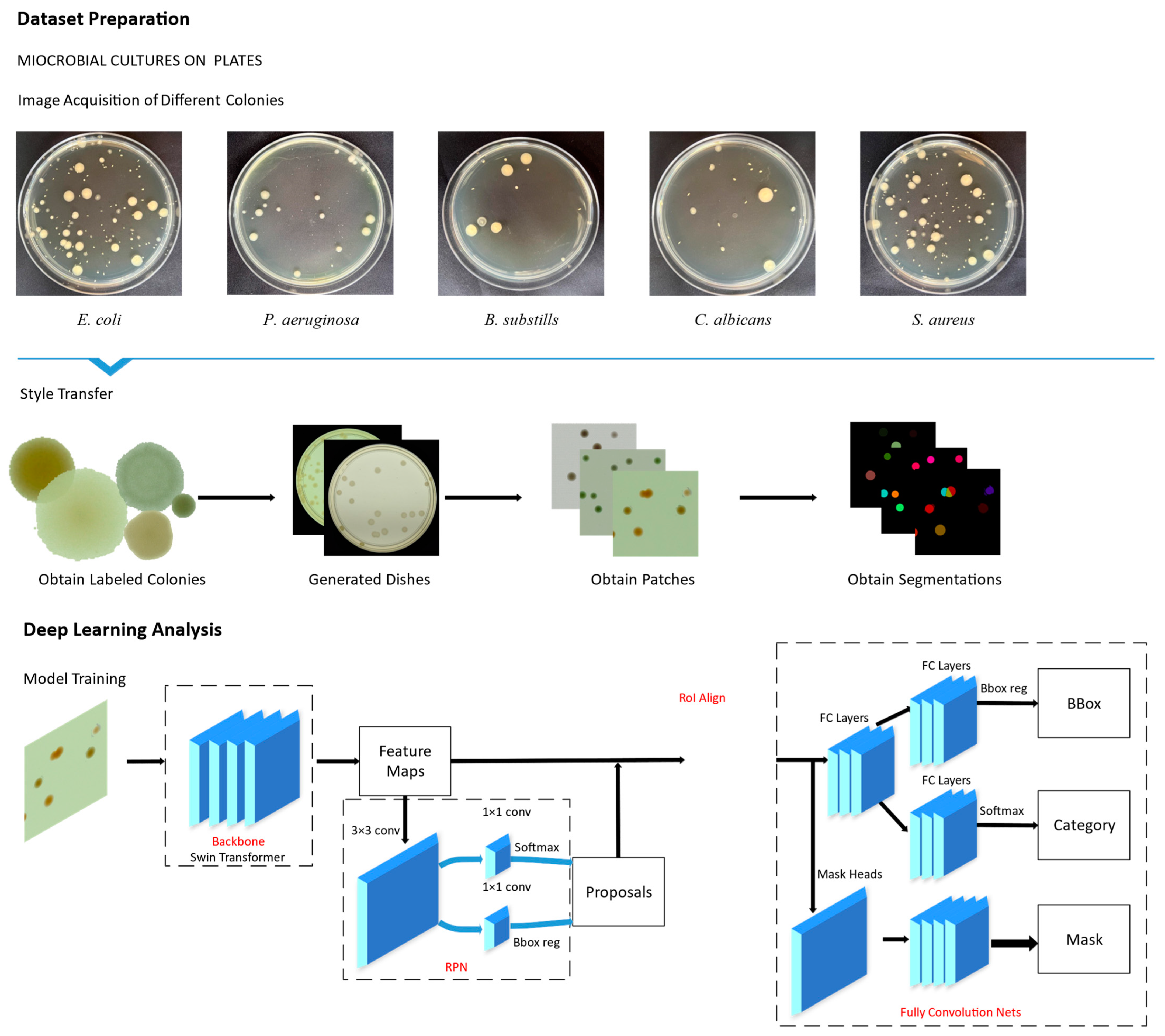
• We propose using style transfer to augment the microbial colony dataset, addressing challenges in acquisition due to contamination and unclear images, and reducing the manual effort required for handling a large number of colonies in the images.
• We combine style transfer and Swin Transformer for object detection on the AGAR datasets, where style transfer generates 4k images used for subsequent model training.
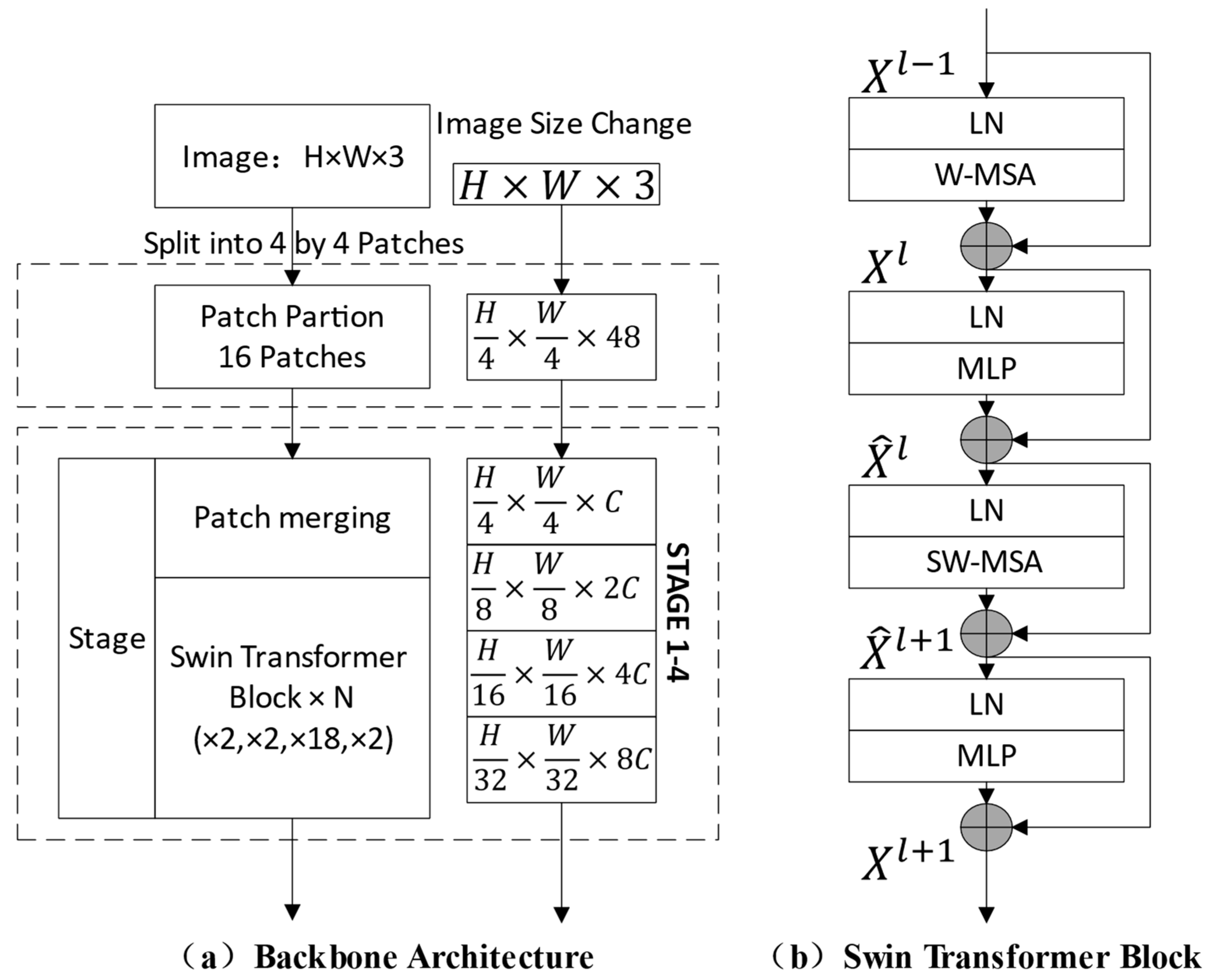
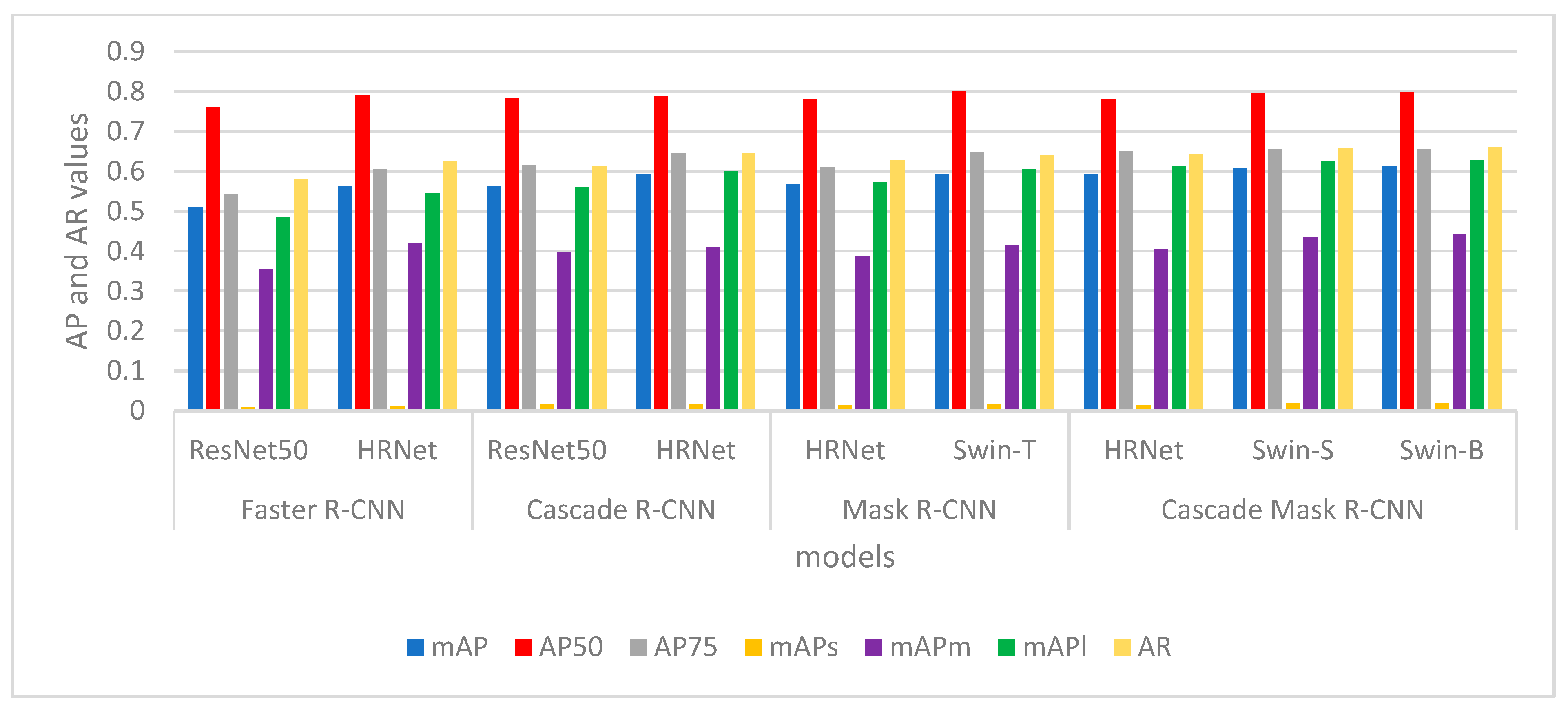
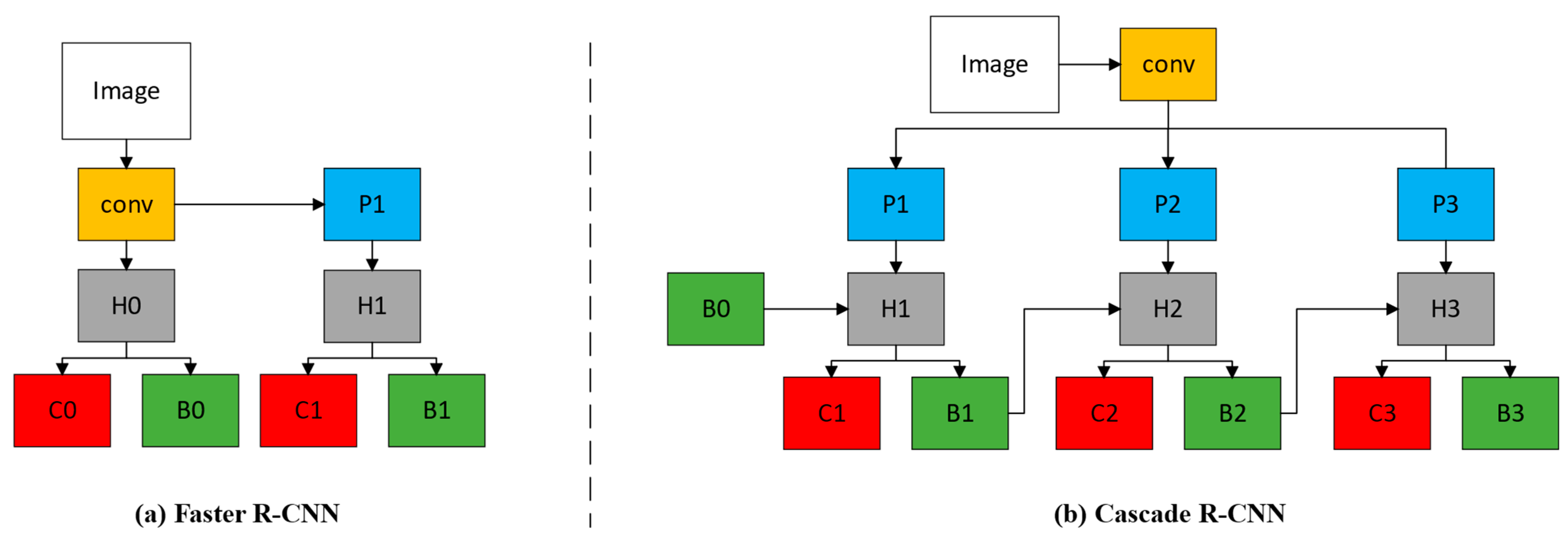
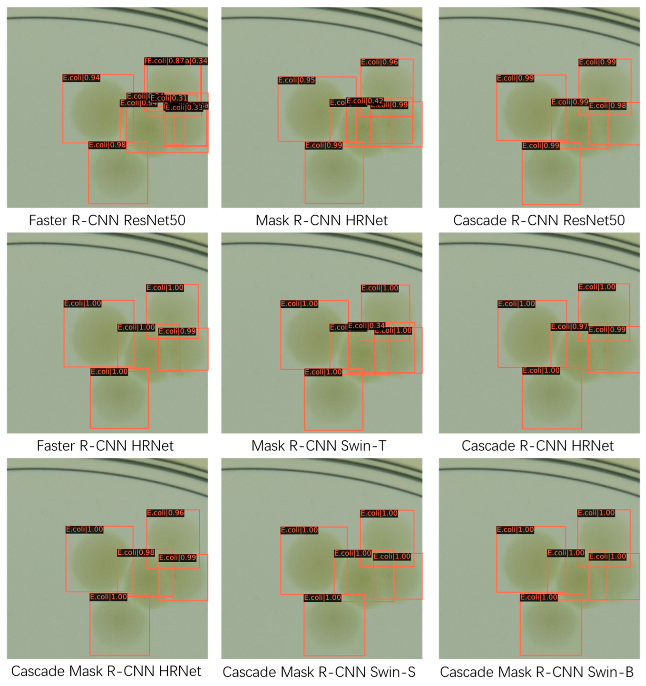
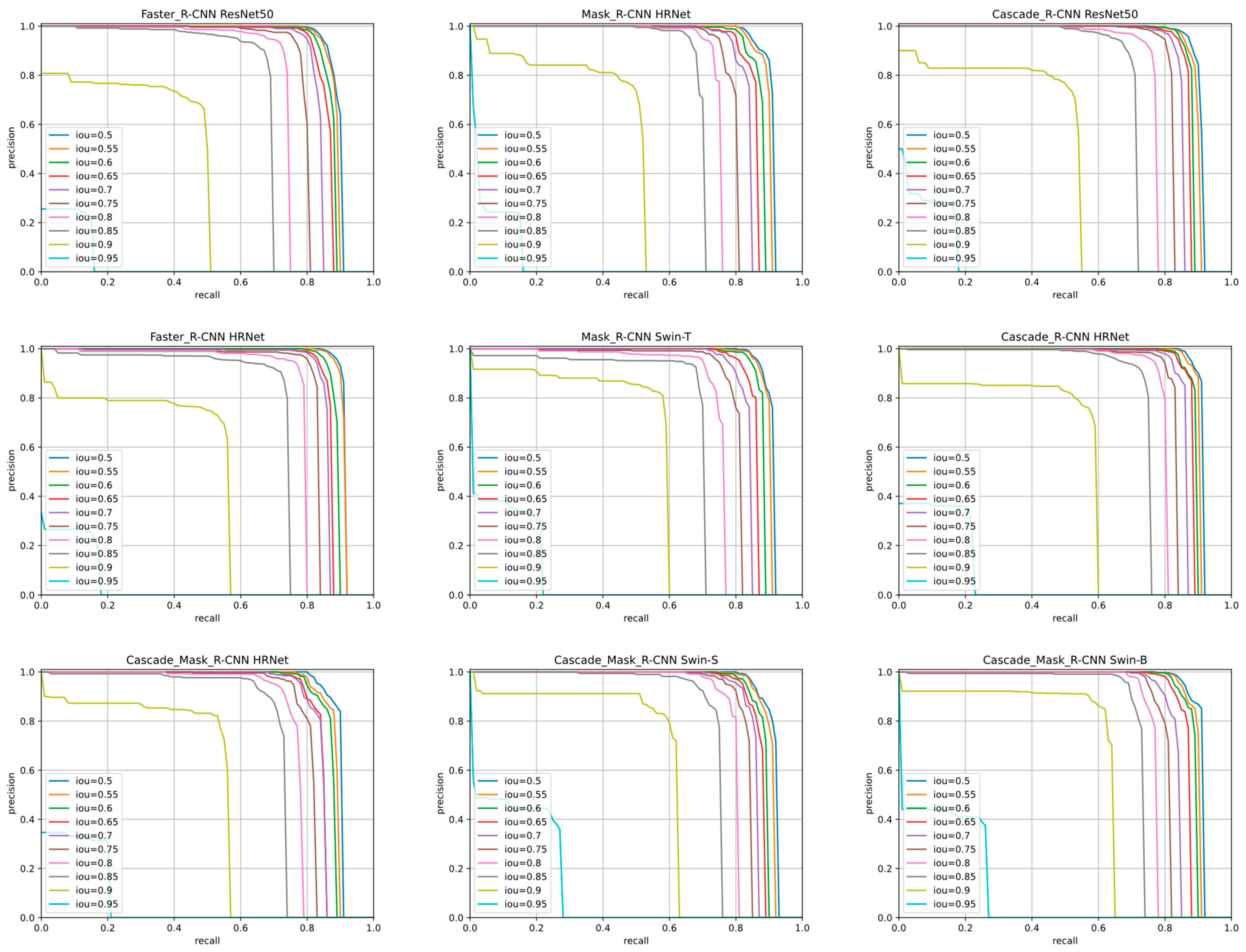
• We compare the model results of Faster R-CNN, Mask R-CNN, Cascade R-CNN, and Cascade Mask R-CNN with High-Resolution Network (HRNet) [23] and Swin Transformer backbone, and use the mAP, AR, etc., as the evaluation metrics for the model. While the traditional Transformer performs self-attentive computation on the entire input sequence, the Swin Transformer introduces a hierarchical attention mechanism. It decomposes the image into multiple small non-overlapping blocks and performs the self-attentive computation on these blocks. This layered design reduces the computational complexity and enables better handling of large-sized images.

The rest of this paper is organized as follows: Section 2 presents the model architectures that are commonly used for object detection with the recent developments and related work on microbial colony identification. Section 3 focuses on the dataset used in this paper and the principles of style transfer and Swin Transformer. Section 4 describes the experimental environment configuration and evaluation metrics and gives the experimental comparison results, which are analyzed and illustrated. Section 5 concludes the work and experimental results of the full paper and describes possible directions for future research.

2. Related Work

2.1. Object Detection

There have been multiple significant advancements in the field of object detection in recent years with the introduction of deep learning-based techniques [24]. The current deep learning-based object detection techniques can be divided into two categories: one-stage object detection algorithms and two-stage object detection algorithms. The one-stage architectures predict classes and generate bounding box locations directly through a single forward propagation process, e.g., You Only Look Once (YOLO) [25] models and Single Shot Multi-Box Detector (SSD) [26]. The two-stage models [27] cope with the target detection task in two main processes. It first generates proposals, and then classifies and fine-tunes these proposals to achieve target detection and localization.

On the other hand, Region-based Convolutional Neural Networks (R-CNNs) [28] introduced the concept of using region proposals for object detection. Proposed in 2013, R-CNN was one of the pioneering models that addressed the challenge of object detection through a two-stage process. It involves creating region proposals via selective search or a Region Proposal Network (RPN), and then using a CNN to classify and improve the bounding boxes for each proposal. Faster R-CNN [29] uses the Region of Interest (RoI) pooling layer to extract features from the full image in order to hasten training. Instead of employing the selective search technique to produce region proposals, an RPN is employed in the Faster R-CNN [30] architecture. This makes it possible to drastically cut down on the model’s inference time. In addition to object detection, the Mask R-CNN [31] model, developed by Kaiming He et al. in 2017, adds a new branch for pixel-level semantic segmentation. Compared to Faster R-CNN, Cascade R-CNN [19] uses a cascade architecture that contains multi-stage classifiers and regressors to incrementally improve object detection performance by filtering false positives and refining predictions at each stage.

The introduction of the Transformer model has revitalized various fields of machine learning, including object detection. The encoder component of the Transformer [32] breaks the image up into small patches for object detection and then encodes each patch into a fixed-dimensional representation. By adding heads after the encoder, the features of each image block are fused using a fully connected layer, resulting in an output feature map that acts as an overall image abstraction. This transformation enables the Transformer to replace traditional CNN-based feature extraction in target detection tasks, offering potential benefits for feature learning and performance improvement.

Facebook AI research introduces an end-to-end Transformer (DETR) [33] architecture that changes the object identification issue into an ensemble prediction problem by skipping anchor frames and Non-Maximum Suppression (NMS) [34] operations in traditional detection. Liu et al. [17] propose local self-attention mechanisms and stage features to deal with large-scale images, use the Swin operation to reduce complexity, and expand the sensory field through different stages. Furthermore, Transformer in Transformer (TNT) [35] proposes a way to nest another small Transformer block inside the Transformer encoder to learn the feature representation at a finer granularity.

YOLOv8 is a state-of-the-art (SOTA) model released by the Ultralytics team in 2023, building upon the success of previous YOLO [36] releases to enhance both performance and flexibility. As a one-stage object detection model, YOLOv8 offers improved speed and accuracy in detection, and it supports multiple tasks, including object detection, instance segmentation, and image classification.

2.2. Microbial Colony Identification

Microbial colony identification has been the focus of in-depth research, and a variety of methodologies have been investigated to achieve the accurate and automated recognition of microbial colonies. In the early stages of research, traditional non-deep learning methods were widely used for this purpose. These methods involved handcrafted features and classical machine learning algorithms to classify and count microbial colonies based on their visual characteristics [37,38].

However, with the emergence of deep learning, there has been a shift towards leveraging its powerful capabilities in microbial colony identification. In particular, CNNs have shown astonishing performance in picture identification tasks. Researchers have applied CNN-based approaches to classify and count microbial colonies, using CNNs’ capacity to automatically extract discriminative features from data [39].

Comparative studies have also been conducted to assess the effectiveness of deep learning methods in comparison to traditional approaches. These studies have highlighted the advantages of deep learning in achieving higher accuracy and robustness compared to traditional methods, while also acknowledging the insights provided by traditional feature engineering techniques [40].

Overall, deep learning algorithms have changed the field of microbial colony identification by allowing for more precise and automated assessments. The combination of classical methodologies and deep learning advancements has significantly advanced the field of identifying microbial colonies, offering valuable solutions for applications in microbiology, agriculture, and healthcare.

3. Materials and Methods

3.1. The Dataset

Our work aims to achieve microbial colony identification. The right growth conditions must be provided (applied medium, incubation temperature and time, culture dilution factors, etc.), and the environment must be ready for raw image acquisition (suitable light source position, light source intensity, or camera type). Therefore, we start our experiments using the AGAR dataset. The microorganism species that we study include B. subtilis, C. albicans, E. coli, P. aeruginosa, and S. aureus, while annotated information includes the number and type of microbial colonies and coordinates of the bounding boxes.

In this paper, we use style transfer for data argumentation on high-resolution raw data images. First, we use these images with the high-resolution raw dataset, which is annotated as input. Second, we set the VGG19 pre-trained model as the backbone for extracting features and set HRNet as the up-sampling and down-sampling network. In this process, the neural network extracts style features and content features. The style characteristics reflect the texture, color, and style of the image, while the content features capture the semantic information of the image. Additionally, an optimization method is used to minimize the difference between the input and output images. Since more attention is paid to the target detection of microbial colonies than to the counting of the number of colonies in drug sensitivity experiments, the high-resolution (4000 × 4000 px) raw images can be divided into many patches (512 × 512 px), each of which contains identifiable annotated microbial colonies. Furthermore, these patches will be used as inputs for object detection into the detector for training and recognition.

In this study, we expand the size of the microbial colony dataset and run an experiment on it using the style transfer approach. We take care to minimize redundancy in both the dataset and the training set to mitigate the risk of overfitting when assigning data to the training set. Afterward, we randomly allocate 80% of these images to the training set, 10% to the test set, and 10% to the validation set to train our model. An image and its accompanying mask are both present in each case.

3.2. Style Transfer

The pipeline of style transfer is depicted in Figure 1. To begin, we utilize the original dataset and pass it through the pre-trained VGG19 model, which consists of 16 convolutional layers and 5 pooling layers. The lower convolutional layers, which focus on capturing image details and texture information, provide content feature representations. By comparing these features with the corresponding layers of the generated image, we establish the content loss, denoted as ${\mathcal{L}}_{\mathit{content}}$. On the other hand, the higher convolutional layers, emphasizing global information and abstract features, offer style feature representations. Comparing these style features with the corresponding layers of the generated image helps to determine the style loss, denoted as ${\mathcal{L}}_{style}$.

To achieve an optimal fusion of content and style, we define the total loss, ${\mathcal{L}}_{\mathit{total}}$, as a weighted combination of content loss and style loss, with tunable hyperparameters ($\alpha$ and $\beta$) controlling the balance between the two. This ensures a seamless integration of essential elements from the input image. The loss function we minimize is expressed as follows:

$$L_{total}=\alpha L_{content}+\beta L_{style}$$

(1)

where the weighting parameters for the reconstruction of content and style are $\alpha$ and $\beta$, respectively.

Finally, to reduce the overall loss, we employ optimization using gradient descent. The created image eventually converges to a new image that contains the original content and style information, as the optimization method iteratively changes it.

3.3. Swin Transformer

The pipeline of the backbone is depicted in Figure 2a, illustrating the base version (Swin-B). To handle 2D images, we restructure the image $x\in R^{H\times W\times C}$ into a series of flattened 2D patches, where $H$ stands for the image’s height, $W$ stands for its width, and $C$ stands for its number of channels.

The image is separated into distinct, non-overlapping patches via a patch-splitting module before being sent to the backbone. Each patch is used as a “token”, and its feature is created by joining the RGB values of its individual raw pixels. This feature is used as a linear embedding layer to input the rawest feature information into the network. In our implementation, the Swin Transformer network consists of four stages, and the feature maps extracted in different stages are of varying sizes, capturing different levels of feature granularity at the semantic scale. Each stage consists of patch merging and Swin Transformer blocks. Patch merging works similarly to the pooling layer of the down-sampling process of a CNN. The architecture processes the input image by treating each patch as an individual “token”, as illustrated in Figure 2a. A set patch size of 4 $\times$ 4 is initially selected. A linear embedding layer uses the feature map’s eigenvalues to project them to the C dimension. These tokenized patches are then subjected to the Swin Transformer block. This set of procedures is known as “Stage 1”. The output feature map that is produced is $\frac{H}{4}\times \frac{W}{4}$ in size, which is a down-sampling of four. Patch merging layers reduce the number of tokens as the network becomes deeper to create a hierarchical representation. Before a linear layer is applied to the 4C-dimensional concatenated features, features from each set of 2 × 2 adjacent patches are concatenated in the first patch merge layer. As a result, the output dimension is set to 2C, and the number of tokens is decreased by a factor of 4 (equal to two times the resolution being down-sampled). After that, Swin Transformer blocks are used to modify the features while keeping the resolution at $\frac{H}{8}\times \frac{W}{8}$. The first phase of feature transformation and patch merging is known as “Stage 2”. For “Stage 3” and “Stage 4”, the procedure is then performed again, producing output resolutions of $\frac{H}{16}\times \frac{W}{16}$ and $\frac{H}{32}\times \frac{W}{32}$, respectively. Together, these steps produce a hierarchical representation with feature map resolutions comparable to those of ordinary convolutional networks. Figure 2a illustrates the architecture of Swin-Base (Swin-B), featuring 128 channels in the first hidden layer and a total of 18 layers in Stage 3. In Section 4, various model sizes are employed to delve into the impact of the backbone’s computational complexity. Among these, Swin-Tiny (Swin-T) and Swin-Small (Swin-S) comprise 6 and 18 layers in Stage 3, respectively, with the initial hidden layer containing 96 channels. This adjustment results in variations in their respective theoretical computational complexities (Flops).

Transformer blocks come with a standard Multi-Head Self-Attention (MSA) module that can link contextual data while simultaneously gathering other kinds of feature data. Window-based Multi-Head Self-Attention (W-MSA) and Shifted Window-based Multi-Head Self-Attention (SW-MSA) are used in the Swin Transformer block in place of the traditional MSA module to reduce computational and memory costs. There is no direct self-attention computation between windows, and self-attention computation is only performed within windows; this approach does not need to pay attention to global positional relations and has better performance for large-sized input images. As illustrated in Figure 2b, an SW-MSA module, a 2-layer Multi-Layer Perceptron (MLP), and a Gaussian Error Linear Unit (GELU) nonlinearity make up a Swin Transformer block. Each MSA and MLP module is followed by a residual connection, and each module is preceded by a Layer Normalization (LN).

Additionally, the MSA module of a conventional Transformer block performs global self-attention by figuring out how one token links to other tokens. The issue caused by this global computation process is that as the size of the image resolution increases, the network computational effort grows quadratically. In contrast, W-MSA can effectively reduce computational complexity because it can only use a local window at each place. The image, when divided into $h \times w$ patches, is computationally difficult, as follows:

$$\mathsf{\Omega }\left(\mathrm{MSA}\right)=4hw{C}^2+2{\left(hw\right)}^{2}C$$

(2)

$$\mathsf{\Omega }\left(\mathrm{W}-\mathrm{MSA}\right)=4hw{C}^2+2M^{2}hwC$$

(3)

where M denotes the window size (set to 7 by default). It is very clear that Window-based self-attention is scalable, but global self-attention computation is typically costly for a large $hw$.

Although MSA can utilize localized windows at each position for self-attention computation, its windows at edge locations may extend beyond the boundaries of the input sequence, leading to insufficient capture of boundary information. To address this issue, SW-MSA introduces a shift mechanism that not only computes self-attention within the window, but also ensures better handling of sequence edges. This enhancement improves the overall model’s feature extraction capability, allowing for more effective information capture at the boundaries.

As illustrated in Figure 2b, the Swin Transformer feeds the patch merging-processed feature maps into the W-MSA modules via LayerNorm layers, each of which is residually connected to another LayerNorm layer. The overall process can be represented by the following equation:

$$\widehat{x^l}=\mathrm{W}-\mathrm{MSA}\left(LN\left(x^{l-1}\right)\right)+x^{l-1}$$

(4)

$$x^l=MLP\left(LN\left(\widehat{x^l}\right)\right)+\widehat{x^l}$$

(5)

$$\widehat{x^{l+1}}=\mathrm{SW}-\mathrm{MSA}\left(LN\left(x^l\right)\right)+x^l$$

(6)

$$x^{l+1}=MLP\left(LN\left(\widehat{x^{l+1}}\right)\right)+\widehat{x^{l+1}}$$

(7)

4. Experiment

We use the MMDetection [41] toolkit implementation to conduct our experiments on the AGAR datasets. Models that were pre-trained on ImageNet-1K [42], which is available in the torchvision package of the PyTorch library, are used to establish the backbones’ weights. This experiment can be divided into two steps. We first perform style transfer learning on annotated microbial images by slicing the image of high-resolution dense colonies into multiple patches (512 × 512 px), and the second step is performed with different deep learning models, including Mask R-CNN, Cascade R-CNN, and Cascade Mask R-CNN, with different backbones, e.g., the ResNet, HRNet, and Swin Transformer, for model training and comparison.

4.1. Evaluation Mertric

We use the common evaluation metrics of the COCO [43] dataset as the assessment metrics for colony detection in this experiment. For the tasks of object detection and instance segmentation for the COCO dataset, the most often employed evaluation measures are the Average Precision (AP) and Average Recall (AR).

The Average Precision quantifies the accuracy of the model in detecting various classes of objects at different Intersection over Union (IoU) thresholds. For each category, objects are initially ranked based on the model’s prediction confidence. Subsequently, the accuracy is computed at various IoU thresholds (typically 0.50, 0.55, 0.60, …, 0.95). The AP for that category is then obtained by averaging the accuracies at different IoU thresholds. Finally, the APs for all of the categories are averaged to calculate the mean Average Precision (mAP). The AP metric comprehensively assesses the model’s performance by considering its accuracy across different classes and IoU thresholds, offering valuable insights into its object detection and instance segmentation capabilities. Higher mAP values indicate better detection accuracy and are indicative of a more versatile and effective model for practical applications.

In addition, the AR is another essential metric that is used in object detection to assess the model’s ability to correctly detect targets under different IoU thresholds. The AR measures the degree of coverage of correctly detected targets by the model. Similar to the AP, the AR calculates the accuracy at different IoU thresholds, representing the proportion of correctly detected targets at varying levels of IoU thresholds. By averaging the AR values across different IoU thresholds, we obtain a comprehensive measure of the model’s detection performance. The AR complements the AP in providing a more holistic evaluation of the model’s ability to recall true targets accurately. Together with the AP, the AR offers valuable insights into the model’s overall detection capabilities, making it an important parameter for evaluating object detection models.

Before providing the specific formula for each indicator, it is necessary to establish the meaning of some confusion matrix symbols because many indicators rely on them for computation. TP, TN, FP, and FN stand for true positive, true negative, false positive, and false negative, respectively. As a result, Equation (8) is used to compute the precision rate and Equation (9) is used to obtain the recall rate.

$$Precision=\frac{TP}{TP+FP}$$

(8)

$$Recall=\frac{TP}{TP+FN}$$

(9)

4.2. Training Configuration

The Cascade Mask R-CNN with the Swin Transformer is developed using Pytorch 1.12.1 and Python 3.8.16. The input image size and patch size are set to 512 $\times$ 512 and 4, respectively, for all of the training cases. We train the models with AMD Ryzen 7 6800H CPU, an RTX 3070 Ti graphics card with 8 GB memory, and 16 GB RAM. The model parameters are initialized using the pre-trained weights from ImageNet-1K. In the training phase, we use the AdamW [44] optimizer with a momentum of 0.9, a learning rate of 10⁻⁴, ${\beta }_1$ of 0.9, ${\beta }_2$ of 0.99, a weight decay of 0.05, and 3× schedule (36 epochs) for the backpropagation of Transformer-based models. On the other hand, we use an SGD optimizer with a momentum of 0.9, a learning rate of 0.002, and a weight decay of 10⁻⁴ for ResNet50- and HRNet-based models.

4.3. Analysis and Evaluation

In this section, we discuss the performance of Faster R-CNN, Mask R-CNN, Cascade R-CNN, and Cascade Mask R-CNN using different backbones. The experimental results are shown in

Table 1. Comparison results of Faster R-CNN, Cascade R-CNN, Mask R-CNN, and Cascade Mask R-CNN with ResNet50, HRNet, and Swin Transformer backbone using AGAR dataset. The AP and AR values in bold are the best, and the underlined values are the second best.

Model	Backbone	Flops (G)	Params (M)	mAP	AP50	AP75	mAPs	mAPm	mAPl	AR
Faster R-CNN	ResNet50	50.38	41.14	0.511	0.760	0.542	0.008	0.354	0.484	0.581
	HRNet	70.44	46.90	0.564	0.791	0.605	0.012	0.421	0.545	0.626
Cascade R-CNN	ResNet50	52.41	68.94	0.563	0.783	0.615	0.016	0.397	0.560	0.613
	HRNet	72.47	74.69	0.592	0.789	0.646	0.017	0.409	0.601	0.645
Mask R-CNN	HRNet	122.00	49.52	0.567	0.782	0.611	0.013	0.386	0.572	0.628
	Swin-T	103.85	47.39	0.593	0.801	0.648	0.017	0.414	0.606	0.642
Cascade Mask R-CNN	HRNet	227.15	82.56	0.592	0.782	0.651	0.013	0.406	0.612	0.644
	Swin-S	576.35	105.74	0.609	0.796	0.656	0.018	0.434	0.626	0.659
	Swin-B	613.78	143.77	0.614	0.798	0.655	0.019	0.443	0.628	0.660

Note: AP: at IoU = 0.50:0.05:0.95; AP50: AP at IoU = 0.50; AP75: AP at IoU = 0.75; APs, AP for small objects: area < 32²; APm, AP for medium objects: 32² < area < 96²; APl, AP for large objects: area > 96².

, and we use the Faster R-CNN architecture with ResNet50 as the baseline to evaluate the Swin Transformer, which incorporates the window self-attention mechanism. Additionally, we extend the base model to compare the training performance of Cascade Mask R-CNN with the other architectures in detecting colony objects in images.

Table 1 and Figure 3 summarize the experimental results of different network configurations. The Cascade Mask R-CNN model with Swin-B achieves the highest performance (compared to Cascade Mask R-CNN with HRNet), outperforming the other configurations in mAP (+2.2%), mAPs (+0.6%), mAPm (+3.7%), mAPl (1.6%), and AR (+1.6%). The integration of the Swin Transformer module significantly enhances the model’s accuracy for microbial colony detection. The success of the W-MSA and SW-MSA methods in extracting edge information from feature images is evident, particularly for detecting colonies near the Petri dish edges. The comparative results emphasize the importance of using advanced self-attention mechanisms in object detection, especially for the accurate identification of microbial colonies in complex images.

Experiments on the AGAR dataset are conducted on both Faster R-CNN and Cascade R-CNN. We also repeat the experiments and obtain similar results. Cascade R-CNN is an extension of Faster R-CNN, where a cascade operation is added after RoI Align, as illustrated in Figure 4. The cascade operation involves passing the outputs of the previous level to the next level with an additional classifier. This process is repeated through multiple stages, with each stage refining the bounding box proposals. The cascading of classifiers and bounding box regressors in multiple stages allows for better localization and filtering of proposals, leading to improved accuracy in object detection. From the experimental results, using ResNet50 and HRNet as the backbone, Cascade R-CNN shows 4.9% and 2.8% improvement in the mAP over Faster R-CNN, respectively. Hence, aiming to enhance the detection accuracy further, we employ the Cascade Mask R-CNN model, which incorporates the segmentation component of Mask R-CNN into the Cascade R-CNN framework. To validate the augmentation of detection capabilities, we integrate the Swin Transformer module into this refined model.

We utilize a patch image containing only E. coli colonies as the input and employ the pre-trained experimental models. The comparison results of the predictions from different models are illustrated in Figure 5. By combining these results with the data presented in

Table 2. Five microbial colonies’ average precision results for Faster R-CNN, Cascade R-CNN, Mask R-CNN, and Cascade Mask R-CNN with ResNet50, HRNet, and Swin Transformer backbone using AGAR dataset.

Model	Cascade Mask R-CNN			Mask R-CNN		Cascade R-CNN		Faster R-CNN
Backbone	Swin-B	Swin-S	HRNet	Swin-T	HRNet	HRNet	ResNet50	HRNet	ResNet50
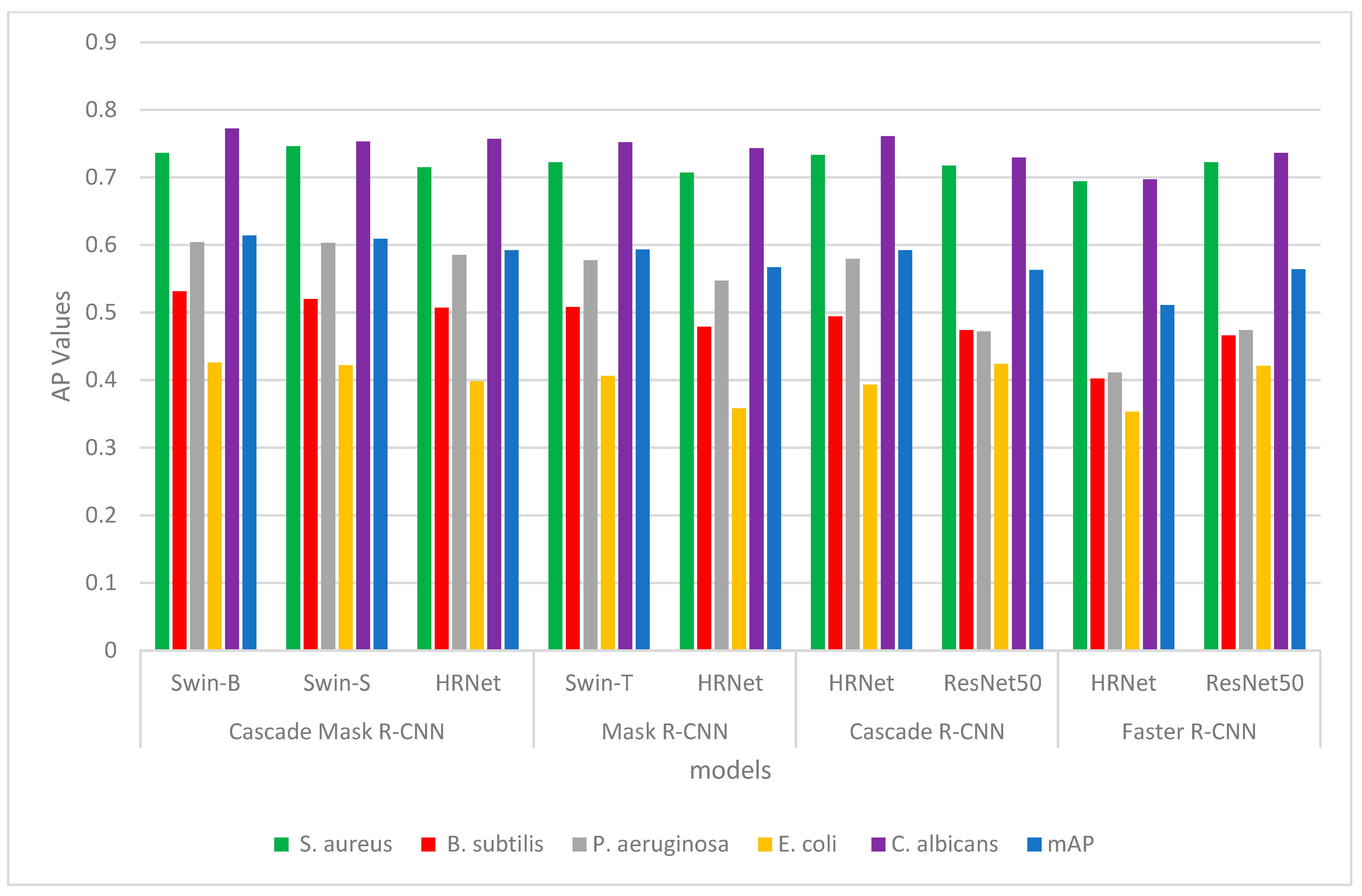
S. aureus	0.736	0.746	0.715	0.722	0.707	0.733	0.717	0.694	0.722
B. subtilis	0.531	0.520	0.507	0.508	0.479	0.494	0.474	0.402	0.466
P. aeruginosa	0.604	0.603	0.585	0.577	0.547	0.579	0.472	0.411	0.474
E. coli	0.426	0.422	0.398	0.406	0.358	0.393	0.424	0.353	0.421
C. albicans	0.772	0.753	0.757	0.752	0.743	0.761	0.729	0.697	0.736
mAP	0.614	0.609	0.592	0.593	0.567	0.592	0.563	0.511	0.564

Note: AP: at IoU = 0.50:0.05:0.95.

and Figure 6, it becomes evident that the detection effects (bounding box and confidence) of the various models on E. coli colonies displayed in the output image are similar to those shown in the AP values table for E. coli. In particular, Faster R-CNN with ResNet50 yields the poorest performance, producing multiple bounding boxes with low confidence in the prediction results. Contrarily, Cascade Mask R-CNN with Swin-S and Swin-B both perform well, demonstrating more consistent prediction results. These findings suggest that deep learning models employing Swin Transformer can indeed improve the accuracy of microbial colony detection to a certain extent.

As depicted in Figure 7, apart from conducting a direct image-based prediction evaluation, we additionally visualize and compare the detection performance of each model by plotting their corresponding PR curves. In these curves, the recall and precision are represented by the horizontal and vertical coordinates, respectively. Higher detection rates and accuracy are shown by the PR curves that are closer to the upper-right corner of the screen. Specifically, we plot the IoU [0.50:0.05:0.95] curves for the different models, and upon observation, we find that the Cascade Mask R-CNN with Swin-B model outperforms the other models in terms of detection accuracy.

As shown in Table 2 and Figure 6, the images of the colony samples that we used in the training model can be categorized into five kinds. Among the different models evaluated, Cascade Mask R-CNN with Swin-B demonstrates superior detection accuracy for each strain of bacteria. In addition, it can be found that the AP calculated for each microbe species reveals that microbes forming smaller colonies, such as S. aureus and C. albicans, achieve higher precision. The other examined microorganisms, however, frequently cluster or overlap, especially in low-dilution samples where more colonies are visible on the plate surface. Additionally, larger colonies frequently have fuzzier edges and less contrast with the agar substrate, which results in less accurate mAP detection. The IoU between the true and predicted bounding boxes is taken into account by the mAP score when evaluating the detection quality. It quantifies the extent of overlap between the ground truth and detected regions, indicating how well the model identifies microbe locations accurately.

In addition to experimenting with the two-stage object detection algorithm, we supplement it with the latest one-stage object detection algorithm, YOLOv8, utilizing YOLOv8x as our pre-trained model. The primary training parameters are detailed in

Table 3. Training parameters and results of experiment on the YOLOv8x model using the AGAR dataset.

Training Settings		Results
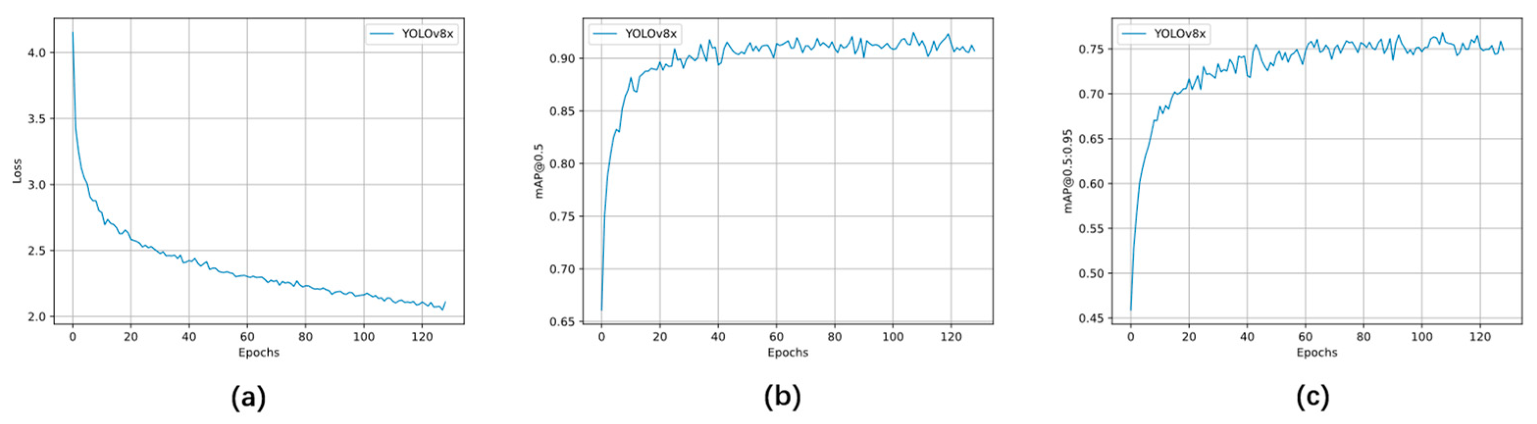
epochs	300	S. aureus	0.849
batch	4	B. subtilis	0.727
iou	0.7	P. aeruginosa	0.696
lr0	0.00001	E. coli	0.698
lrf	0.0001	C. albicans	0.866
momentum	0.9	AP50	0.925
weight decay	0.05	mAP	0.767

. We configure the “patience” parameter to 50, signifying that training would halt if no significant improvement is observed after 50 epochs. Consequently, in practice, the model training concluded at the 129th epoch. The results of the model training are presented in Table 3 and Figure 8. The most outstanding model achieved a mAP of 76.7%, a remarkable 17.5% improvement over the best-performing model (Cascade R-CNN with HRNet) on the AGAR dataset. These results underscore the model’s exceptional performance on the AGAR dataset.

5. Conclusions

In this paper, we propose a new method combining a style transfer extended microbial colony image dataset with a Swin Transformer-based Cascade Mask R-CNN detector for model training. Throughout the experiments, we use Faster R-CNN, Cascade R-CNN, Mask R-CNN, and Cascade Mask R-CNN as the architecture networks and ResNet50, HRNet, and Swin Transformer as the backbone networks to perform the model training and comparison experiments on the AGAR dataset, respectively. The training results indicate that the detector performs well in object detection in microbial colony plate images, with the most accurate being mAP = 0.614, which is 2.2% higher than that of the best performing model of the AGAR dataset experiment (Cascade R-CNN with HRNet). We input microbial colony images into the trained models and assess the detection performance of the various models by analyzing the predictions. The results demonstrate that the Swin Transformer, utilized as a feature extraction network, achieves superior detection results on the microbial colony AGAR dataset. We use YOLOv8x as a pre-trained model, and the results show a mAP of 76.7%. Compared with the two-stage object detection models in this paper, YOLOv8x has a stronger object detection performance, while the experimental results also indicate that it is outstanding in the scenario of microbial colony object detection.

The application of style transfer in the experiments addresses the challenges of fully supervised learning, especially when dealing with imbalanced sources of plate images that might neglect colonies growing at the edges of the Petri dish. The Swin Transformer block, utilized as the model’s feature extraction method, demonstrates excellent performance in the detection results, providing hierarchical features that linearly correlate with the input image. Overall, the findings suggest that the proposed method shows promise in enhancing microbial colony identification in plate images. And we intend to expand our research into additional categories of microbial colony object detection and further explore models such as Cascade Mask R-CNN and YOLOv8.

References

- Tsuchida, S.; Nakayama, T. MALDI-based mass spectrometry in clinical testing: Focus on bacterial identification. Appl. Sci. 2022, 12, 2814. [Google Scholar] [CrossRef]
- Gerhardt, P.; Murray, R.; Costilow, R.; Nester, E.W.; Wood, W.A.; Krieg, N.R.; Phillips, G.B. Manual of Methods for General Bacteriology; American Society for Microbiology: Washington, DC, USA, 1981; Volume 1. [Google Scholar]
- Krizhevsky, A.; Sutskever, I.; Hinton, G.E. Imagenet classification with deep convolutional neural networks. Adv. Neural Inf. Process. Syst. 2012, 25, 1097–1105. [Google Scholar] [CrossRef]
- Cao, B.; Li, C.; Song, Y.; Qin, Y.; Chen, C. Network intrusion detection model based on CNN and GRU. Appl. Sci. 2022, 12, 4184. [Google Scholar] [CrossRef]
- Singh, V.; Gourisaria, M.K.; GM, H.; Rautaray, S.S.; Pandey, M.; Sahni, M.; Leon-Castro, E.; Espinoza-Audelo, L.F. Diagnosis of intracranial tumors via the selective CNN data modeling technique. Appl. Sci. 2022, 12, 2900. [Google Scholar] [CrossRef]
- Beznik, T.; Smyth, P.; de Lannoy, G.; Lee, J.A. Deep learning to detect bacterial colonies for the production of vaccines. Neurocomputing 2022, 470, 427–431. [Google Scholar] [CrossRef]
- Simonyan, K.; Zisserman, A. Very deep convolutional networks for large-scale image recognition. In Proceedings of the 3rd International Conference on Learning Representations (ICLR 2015), San Diego, CA, USA, 7–9 May 2015. [Google Scholar]
- He, K.; Zhang, X.; Ren, S.; Sun, J. Deep Residual Learning for Image Recognition. In Proceedings of the 2016 IEEE Conference on Computer Vision and Pattern Recognition (CVPR), Las Vegas, NV, USA, 27–30 June 2016; p. 770. [Google Scholar]
- Tan, M.; Le, Q.V. EfficientNet: Rethinking Model Scaling for Convolutional Neural Networks. In International Conference on Machine Learning; PMLR: London, UK, 2019; pp. 6105–6114. [Google Scholar]
- Vaswani, A.; Shazeer, N.; Parmar, N.; Uszkoreit, J.; Jones, L.; Gomez, A.N.; Kaiser, Ł.; Polosukhin, I. Attention is all you need. Adv. Neural Inf. Process. Syst. 2017, 30, 5998–6008. [Google Scholar]
- Han, K.; Wang, Y.; Chen, H.; Chen, X.; Guo, J.; Liu, Z.; Tang, Y.; Xiao, A.; Xu, C.; Xu, Y. A Survey on Vision Transformer. IEEE Trans. Pattern Anal. Mach. Intell. 2023, 45, 87–110. [Google Scholar] [CrossRef]
- Zhang, J.; Ma, P.; Jiang, T.; Zhao, X.; Tan, W.; Zhang, J.; Zou, S.; Huang, X.; Grzegorzek, M.; Li, C. SEM-RCNN: A squeeze-and-excitation-based mask region convolutional neural network for multi-class environmental microorganism detection. Appl. Sci. 2022, 12, 9902. [Google Scholar] [CrossRef]
- Gillioz, A.; Casas, J.; Mugellini, E.; Abou Khaled, O. Overview of the Transformer-based Models for NLP Tasks. In Proceedings of the 2020 15th Conference on Computer Science and Information Systems (FedCSIS), Sofia, Bulgaria, 6–9 September 2020; pp. 179–183. [Google Scholar]
- Arnab, A.; Dehghani, M.; Heigold, G.; Sun, C.; Lučić, M.; Schmid, C. ViViT: A Video Vision Transformer. In Proceedings of the 2021 IEEE/CVF International Conference on Computer Vision (ICCV), Virtual, 11–17 October 2021; pp. 6816–6826. [Google Scholar]
- Hu, X.; Li, T.; Zhou, T.; Liu, Y.; Peng, Y. Contrastive learning based on transformer for hyperspectral image classification. Appl. Sci. 2021, 11, 8670. [Google Scholar] [CrossRef]
- Kolesnikov, A.; Dosovitskiy, A.; Weissenborn, D.; Heigold, G.; Uszkoreit, J.; Beyer, L.; Minderer, M.; Dehghani, M.; Houlsby, N.; Gelly, S. An Image is Worth 16 × 16 Words: Transformers for Image Recognition at Scale. arXiv 2021, arXiv:2010.11929. [Google Scholar]
- Liu, Z.; Lin, Y.; Cao, Y.; Hu, H.; Wei, Y.; Zhang, Z.; Lin, S.; Guo, B. Swin Transformer: Hierarchical Vision Transformer using Shifted Windows. In Proceedings of the IEEE/CVF International Conference on Computer Vision, New Orleans, LA, USA, 18–24 June 2022. [Google Scholar]
- Liu, Z.; Hu, H.; Lin, Y.; Yao, Z.; Xie, Z.; Wei, Y.; Ning, J.; Cao, Y.; Zhang, Z.; Dong, L. Swin Transformer V2: Scaling Up Capacity and Resolution. In Proceedings of the 2022 IEEE/CVF Conference on Computer Vision and Pattern Recognition (CVPR), New Orleans, LA, USA, 18–24 June 2022; pp. 11999–12009. [Google Scholar]
- Cai, Z.; Vasconcelos, N. Cascade R-CNN: High quality object detection and instance segmentation. IEEE Trans. Pattern Anal. Mach. Intell. 2019, 43, 1483–1498. [Google Scholar] [CrossRef]
- Wang, C.; Xia, Y.; Liu, Y.; Kang, C.; Lu, N.; Tian, D.; Lu, H.; Han, F.; Xu, J.; Yomo, T. CleanSeq: A pipeline for contamination detection, cleanup, and mutation verifications from microbial genome sequencing data. Appl. Sci. 2022, 12, 6209. [Google Scholar] [CrossRef]
- Majchrowska, S.; Pawlowski, J.; Gula, G.; Bonus, T.; Hanas, A.; Loch, A.; Pawlak, A.; Roszkowiak, J.; Golan, T.; Drulis-Kawa, Z. AGAR a Microbial Colony Dataset for Deep Learning Detection. arXiv 2021, arXiv:2108.01234. [Google Scholar]
- Gatys, L.; Ecker, A.; Bethge, M. A Neural Algorithm of Artistic Style. J. Vis. 2016, 16, 326. [Google Scholar] [CrossRef]
- Wang, J.; Sun, K.; Cheng, T.; Jiang, B.; Deng, C.; Zhao, Y.; Liu, D.; Mu, Y.; Tan, M.; Wang, X. Deep high-resolution representation learning for visual recognition. IEEE Trans. Pattern Anal. Mach. Intell. 2020, 43, 3349–3364. [Google Scholar] [CrossRef]
- Murthy, C.B.; Hashmi, M.F.; Bokde, N.D.; Geem, Z.W. Investigations of object detection in images/videos using various deep learning techniques and embedded platforms—A comprehensive review. Appl. Sci. 2020, 10, 3280. [Google Scholar] [CrossRef]
- Redmon, J.; Divvala, S.; Girshick, R.; Farhadi, A. You Only Look Once: Unified, Real-Time Object Detection. In Proceedings of the IEEE Conference on Computer Vision and Pattern Recognition, Las Vegas, NV, USA, 27–30 June 2016. [Google Scholar]
- Liu, W.; Anguelov, D.; Erhan, D.; Szegedy, C.; Reed, S.; Fu, C.-Y.; Berg, A.C. SSD: Single Shot MultiBox Detector. In Proceedings of the Computer Vision–ECCV 2016: 14th European Conference, Amsterdam, The Netherlands, 11–14 October 2016; Springer International Publishing: Cham, Switzerland, 2016. [Google Scholar]
- Ibrokhimov, B.; Kang, J.-Y. Two-stage deep learning method for breast cancer detection using high-resolution mammogram images. Appl. Sci. 2022, 12, 4616. [Google Scholar] [CrossRef]
- JitendraMalik, R.J.T. Rich Feature Hierarchies for Accurate Object Detection and Semantic Segmentation; ACM: New York, NY, USA, 2014. [Google Scholar]
- Girshick, R. Fast R-CNN. In Proceedings of the 2015 IEEE International Conference on Computer Vision (ICCV), Santiago, Chile, 7–13 December 2015; p. 1440. [Google Scholar]
- Ren, S.; He, K.; Girshick, R.; Sun, J. Faster r-cnn: Towards real-time object detection with region proposal networks. Adv. Neural Inf. Process. Syst. 2015, 28, 1137–1149. [Google Scholar] [CrossRef]
- He, K.; Gkioxari, G.; Dollar, P.; Girshick, R. Mask R-CNN. IEEE Trans. Pattern Anal. Mach. Intell. 2020, 42, 386–397. [Google Scholar] [CrossRef]
- Mabrouk, A.; Díaz Redondo, R.P.; Dahou, A.; Abd Elaziz, M.; Kayed, M. Pneumonia detection on chest X-ray images using ensemble of deep convolutional neural networks. Appl. Sci. 2022, 12, 6448. [Google Scholar] [CrossRef]
- Carion, N.; Massa, F.; Synnaeve, G.; Usunier, N.; Kirillov, A.; Zagoruyko, S. End-to-End Object Detection with Transformers. In European Conference on Computer Vision; Springer International Publishing: Cham, Switzerland, 2020. [Google Scholar]
- Bodla, N.; Singh, B.; Chellappa, R.; Davis, L.S. Soft-NMS–Improving Object Detection with One Line of Code. In Proceedings of the IEEE International Conference on Computer Vision, Venice, Italy, 22–29 October 2017. [Google Scholar]
- Han, K.; Xiao, A.; Wu, E.; Guo, J.; Xu, C.; Wang, Y. Transformer in transformer. Adv. Neural Inf. Process. Syst. 2021, 34, 15908–15919. [Google Scholar]
- Hussain, M. YOLO-v1 to YOLO-v8, the Rise of YOLO and Its Complementary Nature toward Digital Manufacturing and Industrial Defect Detection. Machines 2023, 11, 677. [Google Scholar] [CrossRef]
- Patel, S. Bacterial colony classification using atrous convolution with transfer learning. Ann. Rom. Soc. Cell Biol. 2021, 25, 1428–1441. [Google Scholar]
- Wang, H.; Niu, B.; Tan, L. Bacterial colony algorithm with adaptive attribute learning strategy for feature selection in classification of customers for personalized recommendation. Neurocomputing 2021, 452, 747–755. [Google Scholar] [CrossRef]
- Huang, L.; Wu, T. Novel neural network application for bacterial colony classification. Theor. Biol. Med. Model. 2018, 15, 22. [Google Scholar] [CrossRef]
- Zhao, P.; Li, C.; Rahaman, M.M.; Xu, H.; Yang, H.; Sun, H.; Jiang, T.; Grzegorzek, M. A comparative study of deep learning classification methods on a small environmental microorganism image dataset (EMDS-6): From convolutional neural networks to visual transformers. Front. Microbiol. 2022, 13, 792166. [Google Scholar] [CrossRef]
- Chen, K.; Wang, J.; Pang, J.; Cao, Y.; Xiong, Y.; Li, X.; Sun, S.; Feng, W.; Liu, Z.; Xu, J. MMDetection: Open mmlab detection toolbox and benchmark. arXiv 2019, arXiv:1906.07155. [Google Scholar]
- Deng, J.; Dong, W.; Socher, R.; Li, L.-J.; Li, K.; Fei-Fei, L. ImageNet: A Large-Scale Hierarchical Image Database. In Proceedings of the 2009 IEEE Conference on Computer Vision And Pattern Recognition, Miami, FL, USA, 20–25 June 2009. [Google Scholar]
- Lin, T.-Y.; Maire, M.; Belongie, S.; Hays, J.; Perona, P.; Ramanan, D.; Dollár, P.; Zitnick, C.L. Microsoft coco: Common objects in context. In Proceedings of the Computer Vision–ECCV 2014: 13th European Conference, Zurich, Switzerland, 6–12 September 2014; pp. 740–755. [Google Scholar]
- Loshchilov, I.; Hutter, F. Decoupled Weight Decay Regularization. In Proceedings of the International Conference on Learning Representations, Vancouver, BC, Canada, 30 April–3 May 2018. [Google Scholar]