Multivariate Regression Modeling for Coastal Urban Air Quality Estimates

Abstract

Multivariate regression models for real-time coastal air quality forecasting were suggested from 18 to 27 March 2015, with a total of 15 kinds of hourly input data (three-hours-earlier data of PM and gas with meteorological parameters from Kangnung (Korea), associated with two-days-earlier data of PM and gas from Beijing (China)). Multiple correlation coefficients between the predicted and measured PM₁₀, PM_2.5, NO₂, SO₂, CO and O₃ concentrations were 0.957, 0.906, 0.886, 0.795, 0.864 and 0.932 before the yellow sand event at Kangnung, 0.936, 0.982, 0.866, 0.917, 0.887 and 0.916 during the event and 0.919, 0.945, 0.902, 0.857, 0.887 and 0.892 after the event. As the significance levels (p) from multi-regression analyses were less than 0.001, all correlation coefficients were very significant. Partial correlation coefficients presenting the contribution of 15 input variables to 6 output variables using the models were presented for the three periods in detail. Scatter plots and their hourly distributions between the predicted and measured values showed the quite good accuracy of the modeling performance for the current time forecasting of six output values and their high applicability.

1. Introduction

The rapidly increasing consumption of fossil fuels, such as gasoline and coal, due to industrial development in each country and rural urbanization in northeast and southeast Asia results in worse ambient air pollution, which is mainly composed of particulate matter and gases emitted from the vehicles on the road, industries, forest fires, heating and cooking boilers, trash burning and the yellow dust raised from the desert and arid areas [1,2,3,4,5,6]. Various pollutants are very harmful to human health through respiratory diseases, are a multi-faceted health threat to outdoor physical activity and cause worse visibility during long hazy weather [7,8,9,10,11,12].

Sun et al. [13], Darmenova et al. [14], Wang et al. [15], Uno et al. [16] and Choi and Zhang [17] insist that yellow dust, which is also called various names such as Asian dust, dust storm, yellow sand and KOSA is easily caused under a relative humidity of less than 40% near the ground surface of wide arid areas and the desert in northern China and a wind velocity of over 10 m/s for the dust mobilization in spring.

Iwasaka et al. [18] carried out lidar observation to investigate the large depolarization ratio of free tropospheric aerosols over the Taklamakan Desert. Gao et al. [19], Sun [20], Chung et al. [21] and Zhang et al. [22] reported on dust storm frequency in spring and dust deposition on the Chinese Loess Plateau. As a strong northwesterly wind could remove several hundred thousand tons of both sand and dust from the desert and arid areas and those substances were uplifted, about 50% of the dust was accumulated in the desert area’s vicinity and the rest was transported to downwind areas such as Korea and deposited to its ground surface, causing low visibility due to a higher PM concentration [23,24]. Shim et al. [25] insisted that Asian dust particles transported concurrently with anthropogenic pollutants contributed to an elevated PM_2.5 concentration, through aerosol lidar and optical particle counter measurements.

Using numerical models, Lin [26] showed the transport of yellow sand to Taiwan and Uno et al. [27] explained the long-range transport of soil dust from Asia to the tropical North Pacific. Chin et al. [28], Jaffe et al. [29] and McKendry et al. [30] indicated the long-range transport of air pollutants and Asian dust to southern California and western Canada and further analyzed the chemical composition of aerosols.

Many researchers have conducted statistical and artificial neural network modeling research to predict dust concentrations. The previous statistical analyses on the impact of yellow dust in Korea comprised simple regression models. Lee and Chung [31] explained the fractional ratio and correlations of temporal PM₁₀, PM_2.5 and PM₁ at Gangneung that was affected by the transported dust from the Gobi Desert. Bhaskar and Mehta [32] showed the meteorological effect on particulate matters (PM) in Ahmedabad. Similarly, Chung et al. [33], Li et al. [34], Shi et al. [35] and Zhao [36] explained the relationship of PM with meteorological elements in China using multiple regression models without a gas effect.

Kim [37], Lim [38], Choi [39] and Jeon and Son [40] performed air quality prediction using artificial neural network and multivariate regression models in Korea. The predictions by two models with numerical models were very accurate. Instead of a complicated numerical model, a multivariate regression model was devised for real-time prediction of PM₁₀, PM_2.5, NO₂, SO₂, O₃ and CO at Kangnung (Korea), using 3 h-earlier pollution and meteorological data and 2-days-earlier pollution data from Beijing (China).

2. Study Area and Data Analysis

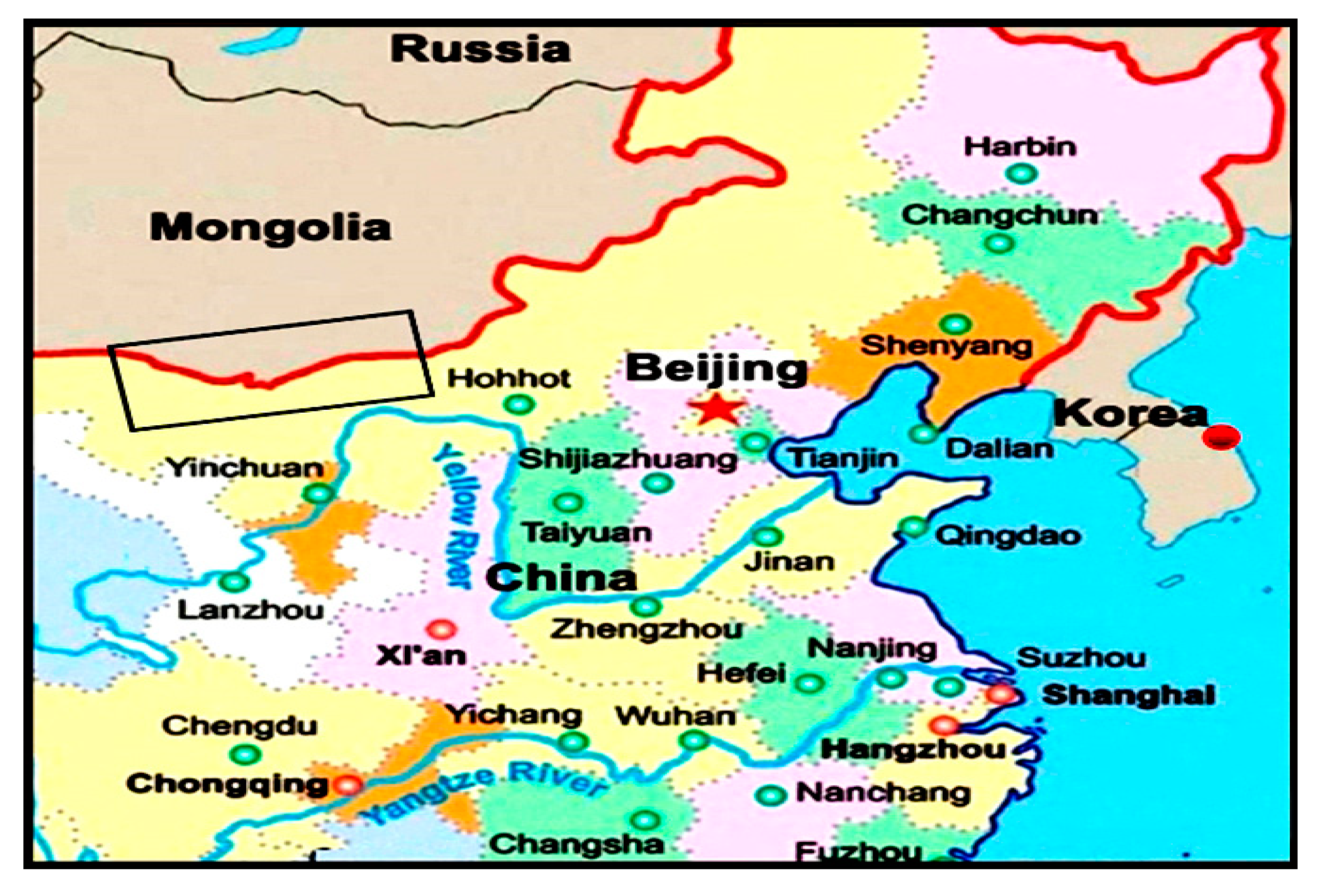
2.1. Study Area

Figure 1 indicates the geographical features of northeastern Asia including Russia, Mongolia (the Gobi Desert), China and Korea.

In spring, when the prevailing northwesterly wind blows over the deserts and arid areas in southern Mongolia and northern China, several hundred thousand tons of sand and dust could be raised up and transported downwind in an eastward direction toward Beijing (China). The dust could combine with local pollutants emitted from Beijing and reach Korea’s eastern coast, including Kangnung City, resulting in a worse influence on its urban air quality.

2.2. Measured Material and Analysis of Data

Hourly averaged PM₁₀, PM_2.5, SO₂, CO, O₃ and NO₂ concentrations measured at the Ockcheondong observation point of Kangnung city were obtained from the homepage (Air Korea) of the Korea Environment Corporation (website address: https://www.airkorea.or.kr/web/, accessed on 1 February 2023) and hourly meteorological data (air temperature (°C; TEMP), wind speed (m/s; WIND) and relative humidity (%; RH)) measured at the Okcheondong observation point of Kangnung city by the Gangwon Regional Meteorological Administration (GRMA) were obtained through a website (https://data.kma.go.kr/, accessed on 1 February 2023). Hourly PM₁₀, PM_2.5, SO₂, CO, O₃ and NO₂ values measured at the Yongdingmen observation point in Beijing, China, were also obtained (https://quotsoft.net/air/, accessed on 20 January 2021).

Uno et al. [16], Choi and Zhang [17] and Kai et al. [18] explained clearly that the yellow dust particles raised from the Gobi Desert under strong northwesterly wind over 10 m/s were transported toward downwind regions such as Beijing and they further combined with local pollutants emitted from the cities. Then, those particles moved to the further downwind regions such as the Korean peninsula including Kangnung city and the islands of Japan. It takes approximately two days (i.e., 48 h) for the particles to travel the over 1400 km distance between Beijing and Kangnung. This means the current concentrations of particulate matter and gases at Kangnung City should be affected by the two-days-earlier air pollutant concentrations in Beijing.

Thus, in this study to make current-time predictions of air pollutant concentrations, such as PM (PM₁₀ and PM_2.5) and gas (SO₂, CO, O₃ and NO₂), at Kangnung City, we used input data sets of not only three-hours-earlier data of PM, gas and meteorological parameters (air temperature, wind speed and relative humidity) at Kangnung city but also two-days-earlier data of PM and gas in Beijing.

The correlation coefficients and regression equations between the observed and predicted PM₁₀, PM_2.5, SO₂, CO, O₃ and NO₂ concentrations at Kangnung City affected by the PM and gases from Beijing city (China) in the yellow sand route between 18 and 27 March were divided into three periods: before the inflow of yellow dust (00:00 LST, 18 March 2015–00:00 LST 21 March 2015), during its inflow (01:00 LST, 21 March 2015–00:00 LST, 23 March 2015) and after its inflow (01:00 LST, 23 March 2015–00:00 LST, 27 March 2015). Thus, multivariate regression prediction models were obtained via multiple regression analyses using SPSS-v27 statistical software. The predicted value of each pollutant was compared with the one later observed to test the goodness of its predicted value.

3. Results

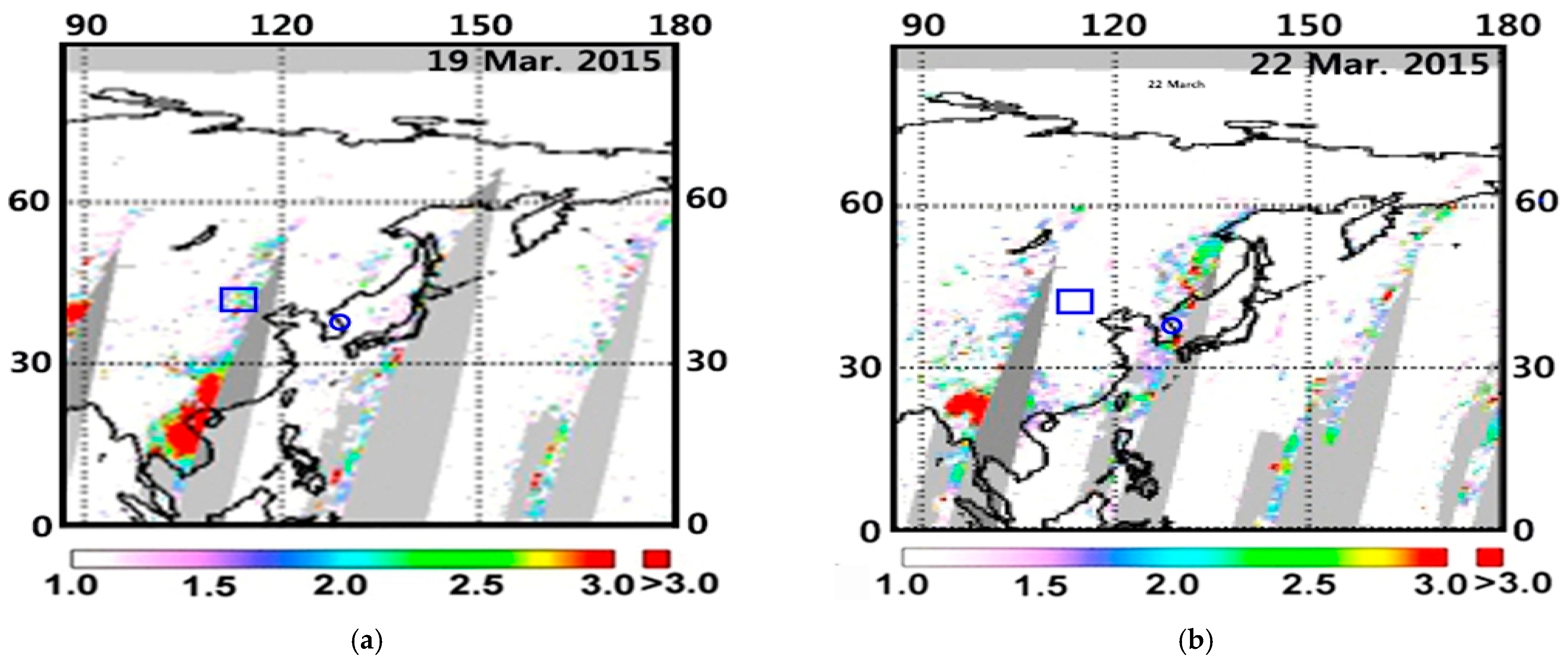
3.1. Satellite Images of Yellow Dust Transport

We used GONE-2 (METOP-B) KNMI/O3MSAF/EUMETSAT satellite images reflecting a cloud of dust before and during yellow sand periods in 2015 to investigate the transport of yellow dust from northern China, including desert and dry areas, to the downwind regions, such as South China, Korea and Japan, in the dust transport route in Figure 2a,b.

Figure 2a shows that the GONE-2 (METOP-B) satellite images can reflect the yellow sand and dust initially raised from the arid areas in the east of Lake Baikal in Siberia (Russia), the Gobi Desert and Inner Mongo in northern China. Then, the dust clouds move toward eastern China, extending to southern China at the same time on 18 March. After that, on 19 March, as shown in Figure 2a, the dust clouds moved further eastward and passed by Beijing and Tianjin, with the dust belt extended to southern China and Vietnam. However, the yellow dust did not reach the Korean peninsula, including the Korean east coast and Kangnung. Another dust belt was detected from Hokkaido in northern Japan to Honshu in the middle of Japan that extended to the east of the Philippines.

In Figure 2b, the METOP-B images show the dust belt from Vladivostok (Russia) to the Korean peninsula, including its east coast (Kangnung city, Republic of Korea), Kyusu Island (Japan), Taiwan and Luzon Island (Philippines) on 22 March, when PM₁₀ concentration was very high at Kangnung during the yellow sand event from 00:01 LST, 21 March to 00:00 LST, 23 March. This dust belt is attributed to the transport of the previous dust belt that was on the line of Beijing–southern China–Vietnam on 19 March in Figure 2a.

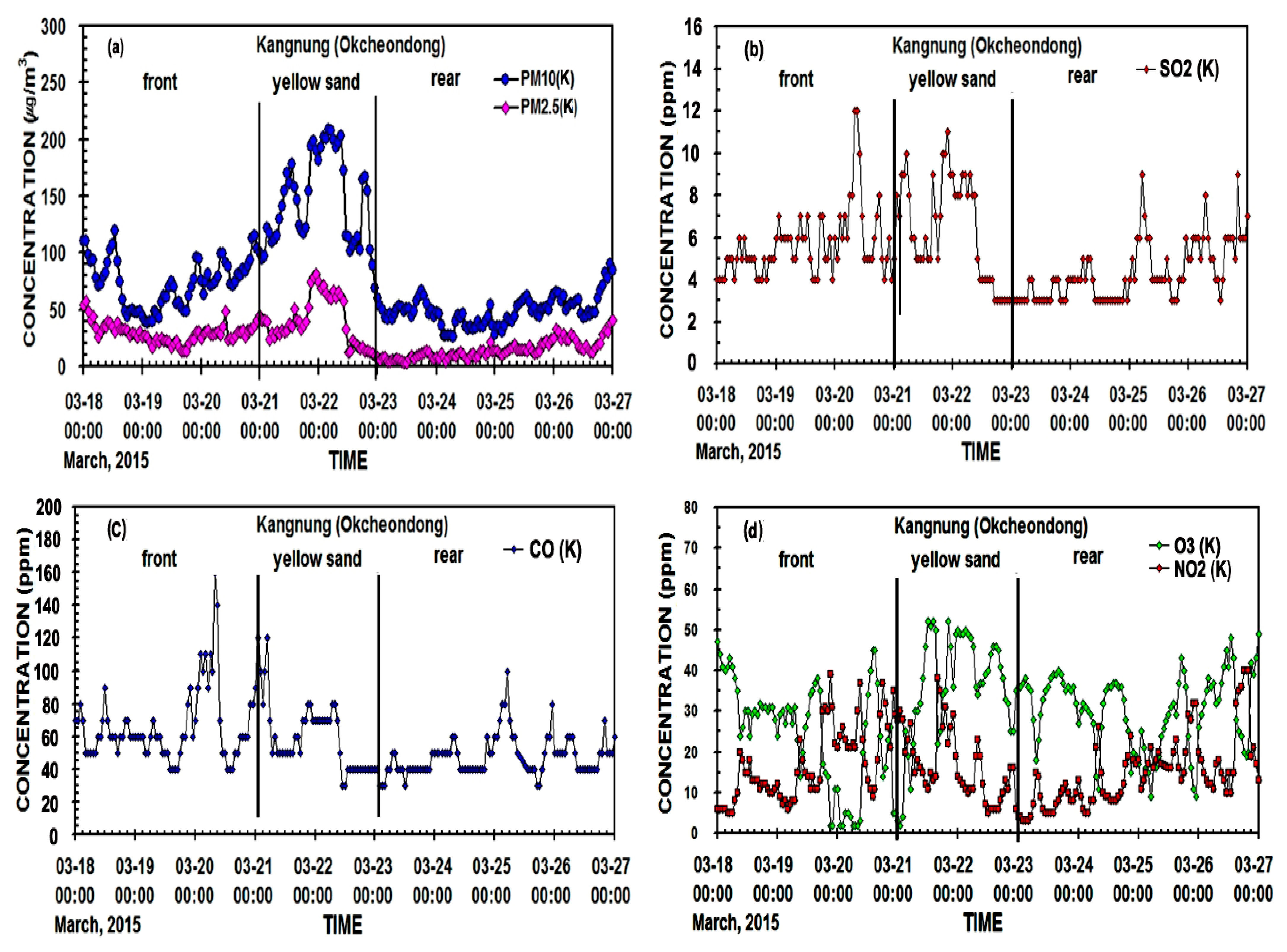
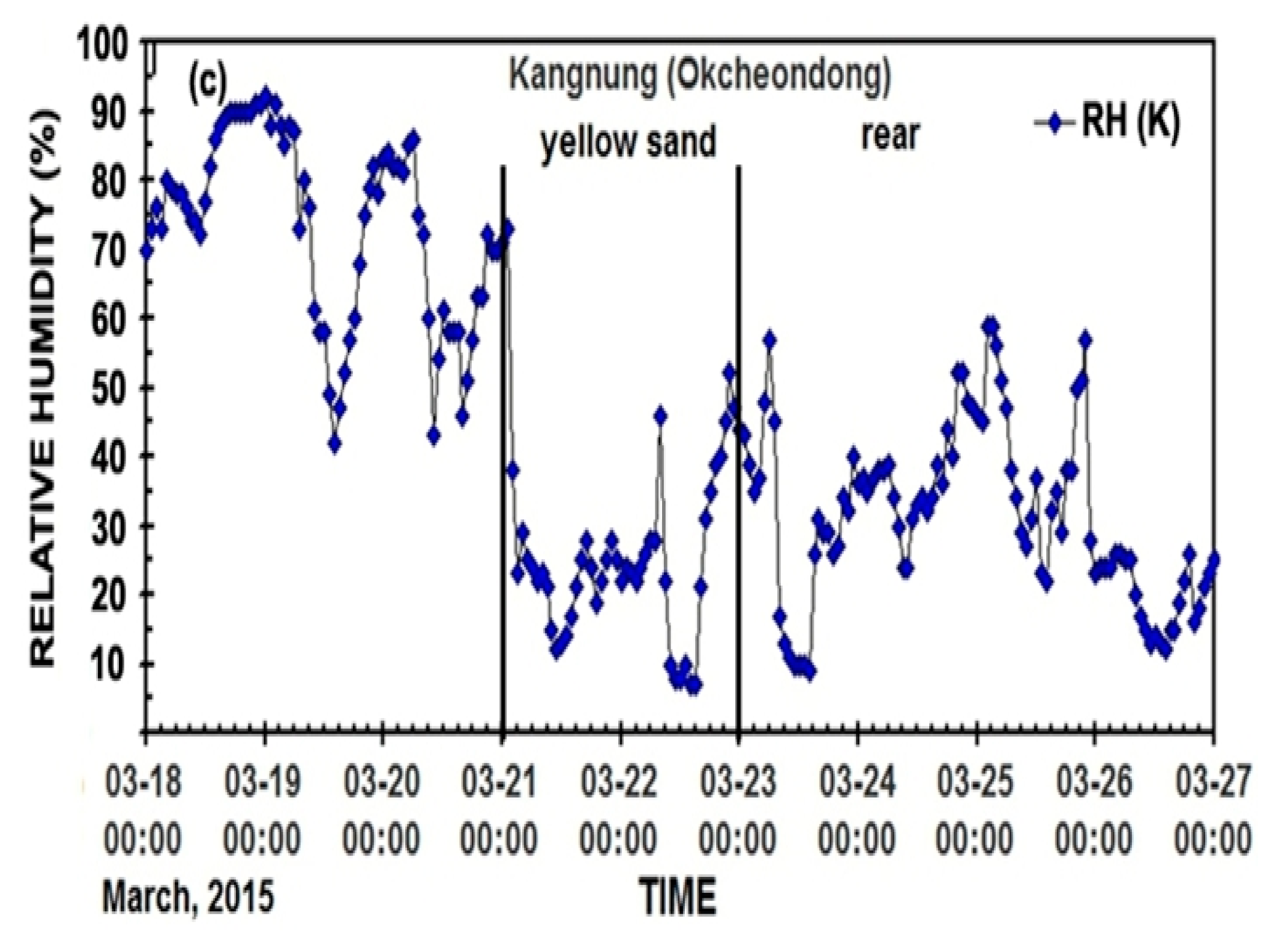
3.2. Hourly PM₁₀, PM_2.5 and PM₁ Concentrations before, during and after the Dust Periods

Figure 3 and Figure 4 indicate the hourly distribution of PM (PM₁₀ and PM_2.5) and gas (SO₂, CO, O₃ and NO₂) concentrations and meteorological parameters (air temperature, wind speed and relative humidity) at the Okcheondong observation point in Kangnung (Korea). Figure 5 also indicates the hourly distribution of PM (PM₁₀ and PM_2.5) and gas (SO₂, CO, O₃ and NO₂) concentrations at the Yongdingmen observation point in Beijing (China).

Choi and Zhang [17] indicated that the transportation of pollutants from Beijing (China) to Kangnung (Korea) takes about two days via a northwesterly wind of about 10 m/s. Thus, PM and gas pollutants for the second sand period in Beijing in Figure 5 may contribute to pollutant concentrations in Kangnung two days later in Figure 3. Thus, PM concentrations for the yellow sand event (on 00 LST, 21 March to 00 LST, 23 March) detected at the Okcheondong observation point in Kangnung could have been affected by PM and gaseous pollution at the Yongdingmen observation point in Beijing two days earlier (00 LST, 19 March to 00 LST, 21 March), corresponding to the second yellow sand period in Beijing.

In Figure 3, the PM₁₀ concentration before the Yellow Sand event at Kangnung was about 50.445 μg/m³. When the PM₁₀ concentration increased, the PM_2.5 concentration increased and had a mean value of 41.234 μg/m³. Both during the event (01:00 LST, 21 March to 00:00 LST, 23 March) and in the early stages after the event on 23 March, the PM₁₀ and PM_2.5 concentrations rapidly increased; however, the increase in PM_2.5 was much smaller than that in PM₁₀. This may be attributed to the intrusion of major coarse particles of yellow sand into Kangnung. After the event, the temporal distributions of PM₁₀ and PM_2.5 had a similar pattern, with similar magnitudes to those values of PM concentrations before the event with slightly different magnitudes.

We further investigated the effect of the ground-based concentrations of SO₂, CO, O₃ and NO₂ at Kangnung in increasing the PM concentrations in Figure 3 before, during and after the yellow sand event from 00 LST, 18 March to 00 LST, 27 March. The SO₂, NO₂ and CO concentrations had a similar temporal tendency to some extent, whereas O₃ had an opposite tendency. The concentrations before and during the event were slightly higher than ones after the event; however, the CO concentration relatively unchanged.

In Figure 3d shows, as Mendez et al [42] explained, that when the O₃ concentration increases, the NO₂ concentration decreases. A diurnal NO_X (= NO₂ + O₃) cycle shows that NOx emitted from the vehicles on the road and heating boilers in residential areas undergoes its photochemical reaction into O₃ due to the increased daytime solar radiation, resulting in its decrease. In contrast, O₃ is reduced to NO₂ at night through the NOx cycle (i.e., no photochemical reaction of NO₂), leading to a decrease in O₃ concentration. Chu et al. [43] insisted that the decreases in PM_2.5 and NO₂ concentrations support the control of NO_x to further reduce PM_2.5 pollution in China and result in the increase in O₃ concentrations.

We investigated whether meteorological parameters could influence PM and gas concentrations for the whole research period in Figure 4. The daytime air temperature near the ground surface during the yellow sand event at Kangnung (from 01:00 LST, 21 March to 00:00 LST 23 March) was much higher than in other periods. The maximum wind speed also became much higher than in other periods. The wind speed should be over 10 m/s (gust wind) for the dust mobilization in the desert. After the dust raised from the desert surface was uplifted to about a 3 km height, it was then transported a by westerly wind of 8 m/s to 10 m/s and moved to the downwind site of Kangnung 1400 km away. When high PM concentrations due to the dust were detected in Beijing, its local wind speed also became higher, with a maximum of 5.8 m/s more than before; however, it was much lower due to the rough mountain topography surrounding the city than it was in the desert.

As the relative humidity had very low values of 6% to 54%, it was very dry without precipitation in Kangnung. During the yellow sand period at Kangnung, the hourly air temperature and wind speed increased more than in other periods but the relative humidity tended to decrease. Thus, these trends for the meteorological parameters may affect the PM and gas concentrations in the city in the presence of absence of yellow sand events.

Figure 5 shows that the SO₂ and CO concentrations during the second yellow sand period in Beijing from 00 LST, March 19 to 00 LST, March 21 decreased more markedly than before and after this period; however, as with the SO₂ and CO concentrations, the NO₂ concentration also slightly decreased but with smaller differences, whereas there was an opposite distribution of O₃ to NO₂ due to the NO_x cycle. Therefore, the gases in Beijing may affect the PM and gas concentrations at Kangnung.

3.3. Definition of Variables in the Multivariate Regression Model

A multivariate regression model consists of a set of independent variables as input data X_j to predict the dependent variable as output data Y_i, as shown in

Table 1. Input and output variables in the multivariate regression model for real-time forecasting.

Input Variable		Output Variable
${\mathrm{X}}_1$	PM10_K: 3 h before	at Kangnung city, Korea ${\mathrm{Y}}_1$ PM10_K(N): present (now) ${\mathrm{Y}}_2$ PM2.5_K(N): present (now) ${\mathrm{Y}}_3$ SO2_K(N): present (now) ${\mathrm{Y}}_4$: CO_K(N): present (now) ${\mathrm{Y}}_5$ O3_K(N): present (now) ${\mathrm{Y}}_6$ NO2+_K(N): present (now)
${\mathrm{X}}_2$	PM2.5_K: 3 h before
${\mathrm{X}}_3$	TEMP_K: 3 h before
${\mathrm{X}}_4$	WIND_K: 3 h before
${\mathrm{X}}_5$	RH_K: 3 h before
${\mathrm{X}}_6$	SO2_K: 3 h before
${\mathrm{X}}_7$	CO_K: 3 h before
${\mathrm{X}}_8$	O3_K: 3 h before
${\mathrm{X}}_9$	NO2_K: 3 h before
${\mathrm{X}}_{10}$	PM10_C: 2 days before
${\mathrm{X}}_{11}$	PM2.5_C: 2 days before
${\mathrm{X}}_{12}$	SO2_C: 2 days before
${\mathrm{X}}_{13}$	CO_C: 2 days before
${\mathrm{X}}_{14}$	O3_C: 2 days before
${\mathrm{X}}_{15}$	NO2_C: 2 days before

. This means that the 15 input variables include data for three hours earlier at Kangnung (PM (PM₁₀-K, PM_2.5-K), meteorological (TEMP_K, WIND_K, RH_K) and gas (SO₂_K, CO_K, O₃_K, NO₂_K)) and for 2 days earlier at Beijing (PM (PM₁₀_C, PM_2.5_C) and gas (SO₂_C, CO_C, O₃_C, NO₂_C)) that were used to make real-time output forecasting variables (PM₁₀_K(N), PM_2.5_K(N), SO₂_K(N), CO_K(N), O₃_K(N) and NO₂_K(N)) at Kangnung.

3.4. Regression Equations and Correlation Matrix among PM₁₀, PM_2.5, SO₂, CO, O₃ and NO₂ Parameters (Kangnung) Affected by Meteorological Variables Associated with PM and Gases (Beijing)

A multiple regression equation consists of independent variables X_j to predict the dependent variable Y_i, such as in Equations (1) and (2).

Y1 = a11X1 + a12X2 + a13X3 + a14X4 + a15X5 + a16X6 + a17X7 + a18X8 + a19X9 + a110X10 + a111X11 + a112X12 + a113X13 + a114X14 + a115X15 + b1 Y2 = a21X1 + a22X2 + a23X3 + a24X4 + a25X5 + a26X6 + a27X7 + a28X8 + a29X9 + a210X10 + a211X11 + a212X12 + a213X13 + a214X14 + a215X15 + b2 Y3 = a31X1 + a32X2 + a33X3 + a34X4 + a35X5 + a36X6 + a37X7 + a38X8 + a39X9 + a310X10 + a311X11 + a312X12 + a313X13 + a314X14 + a315X15 + b3 Y4 = a41X1 + a12X2 + a13X3 + a14X4 + a15X5 + a16X6 + a17X7 + a18X8 + a19X9 + a110X10 + a111X11 + a112X12 + a113X13 + a114X14 + a115X15 + b1 Y5 = a51X1 + a22X2 + a23X3 + a24X4 + a25X5 + a26X6 + a27X7 + a28X8 + a29X9 + a210X10 + a211X11 + a212X12 + a213X13 + a214X14 + a215X15 + b2 Y6 = a61X1 + a32X2 + a33X3 + a34X4 + a35X5 + a36X6 + a37X7 + a38X8 + a39X9 + a310X10 + a311X11 + a312X12 + a313X13 + a314X14 + a315X15 + b3

(1)

Equation (1) can be rewritten in a matrix form as below.

$$\left[\begin{array}{c}{\mathrm{Y}}_1\\ {\mathrm{Y}}_2\\ {\mathrm{Y}}_3\\ {\mathrm{Y}}_4\\ {\mathrm{Y}}_5\\ {\mathrm{Y}}_6\end{array}\right]=\left[\begin{array}{c}{\mathrm{a}}_{11 }{\mathrm{a}}_{12 }\dots \dots \dots \dots {\mathrm{a}}_{115}\\ {\mathrm{a}}_{21} {\mathrm{a}}_{22} \dots \dots \dots \dots {\mathrm{a}}_{215}\\ {\mathrm{a}}_{31} {\mathrm{a}}_{32} \dots \dots \dots \dots {\mathrm{a}}_{315}\\ {\mathrm{a}}_{41} {\mathrm{a}}_{42} \dots \dots \dots \dots {\mathrm{a}}_{415}\\ {\mathrm{a}}_{51} {\mathrm{a}}_{52} \dots \dots \dots \dots {\mathrm{a}}_{515}\\ {\mathrm{a}}_{61} {\mathrm{a}}_{62} \dots \dots \dots \dots {\mathrm{a}}_{615}\end{array}\right]\left[\begin{array}{c}{\mathrm{X}}_1\\ {\mathrm{X}}_2\\ {\mathrm{X}}_3\\ {\mathrm{X}}_4\\ {\mathrm{X}}_5\\ {\mathrm{X}}_6\\ {\mathrm{X}}_7\\ {\mathrm{X}}_8\\ {\mathrm{X}}_9\\ {\mathrm{X}}_{10}\\ {\mathrm{X}}_{11}\\ {\mathrm{X}}_{12}\\ {\mathrm{X}}_{13}\\ {\mathrm{X}}_{14}\\ {\mathrm{X}}_{15} \end{array}\right]+\left[\begin{array}{c}{\mathrm{b}}_1\\ {\mathrm{b}}_2\\ {\mathrm{b}}_3\\ {\mathrm{b}}_4\\ {\mathrm{b}}_5\\ {\mathrm{b}}_6\end{array}\right]$$

(2)

where a_ij (i = 1 to 6; j = 1 to 15) indicates the coefficient of the matrix and the measured values of X_j (j; represents the number of independent variables; j = 1 to 15) such as PM₁₀_K, PM_2.5_K, TEMP_K (air temperature), WIND_K (wind speed), RH_K (relative humidity), SO₂_K, CO_K, O₃_K, NO₂_K, PM₁₀_C, PM_2.5_C, SO₂_C, CO_C, O₃_C and NO₂_C. The real-time predictive values Y_i (i = 1 to 6; PM₁₀_K(N), PM_2.5_K(N), SO₂_K(N), CO_K(N), O₃_K(N) and NO₂_K(N)) are dependent variables and b_i (i = 1 to 6) is an error term that intercepts in the equations of Y_i.

In this study, our prediction models comprise multiple predictive regression equations on each PM₁₀_K, PM_2.5_K, SO₂_K, CO_K, O₃_K and NO₂_K value that are influenced by not only meteorological and gas parameters of the city but also PM₁₀_C, PM_2.5_C, SO₂_C, CO_C, O₃_C and NO₂_C concentrations.

Table 2. Multivariate correlation coefficients and predictive regression equations for real-time PM₁₀_K(N), PM_2.5_K(N), SO₂_K(N), CO_K(N), O₃_K(N) and NO₂_K(N) values at Kangnung, Korea (K) affected by meteorological parameters associated with the PM and gases in Beijing, China (C) before the Yellow Sand event, 2015.

Period	Multi-Correlation Coefficient (r)	Multivariate Predictive Regression Equation
18–21 March 2015 before the Yellow Sand Event	0.957	PM10_K(N)	=	0.559 × PM10_K − 0.175 × PM2.5_K + 2.362 × TEMP_K − 1.355 × WIND_K − 0.477 × RH_K
				− 2.982 × SO2_K + 0.162 × CO_K − 0.143 × O3_K + 0.304 × NO2_K + 0.036 × PM10_C
				− 0.036 × PM2.5_C + 0.340 × SO2_C − 0.064 × CO_C − 0.500 × O3_C − 0.148 × NO2_C + 87.948
	0.906	PM2.5_K(N)	=	0.122 × PM10_K + 0.452 × PM2.5_K − 0.164 × TEMP_K + 0.291 × WIND_K + 0.204 × RH_K
				− 0.257 × SO2_K + 0.148 × CO_K + 0.526 × O3_K + 0.565 × NO2_K + 0.002 × PM10_C
				− 0.008 × PM2.5_C − 0.075 × SO2_C + 0.013 × CO_C + 0.005 × O3_C + 0.006 × NO2_C − 37.838
	0.886	NO2_K(N)	=	0.001 × PM10_K − 0.058 × PM2.5_K − 0.332 × TEMP_K − 1.788 × WIND_K + 0.194 × RH_K
				+ 0.407 × SO2_K − 0.016 × CO_K + 0.156 × O3_K + 0.784 × NO2_K + 0.001 × PM10_C
				− 0.019 × PM2.5_C − 0.070 × SO2_C − 0.006 × CO_C + 0.124 × O3_C + 0.153 × NO2_C − 19.762
	0.795	SO2_K(N)	=	−0.013 × PM10_K − 0.012 × PM2.5_K + 0.196 × TEMP_K − 0.415 × WIND_K + 0.030 × RH_K
				+ 0.521 × SO2_K + 0.009 × CO_K − 0.040 × O3_K − 0.065 × NO2_K − 0.007 × PM10_C
				+ 0.003 × PM2.5_C + 0.021 × SO2_C − 0.001 × CO_C − 0.001 × O3_C + 0.016 × NO2_C + 1.682
	0.932	O3_K(N)	=	−0.033 × PM10_K + 0.012 × PM2.5_K + 1.353 × TEMP_K + 2.838 × WIND_K − 0.218 × RH_K
				+ 0.111 × SO2_K + 0.043 × CO_K + 0.564 × O3_K − 0.221 × NO2_K + 0.001 × PM10_C
				+ 0.022 × PM2.5_C + 0.183 × SO2_C + 0.001 × CO_C − 0.172 × O3_C − 0.182 × NO2_C + 26.519
	0.864	CO_K(N)	=	−0.033 × PM10_K + 0.423 × PM2.5_K + 0.141 × TEMP_K + 1.200 × WIND_K + 0.235 × RH_K
				− 0.412) × SO2_K + 0.372 × CO_K − 1.404) × O3_K − 1.510) × NO2_K + 0.073 × PM10_C
				− 0.096) × PM2.5_C − 0.056) × SO2_C − 0.068) × CO_C + 0.025 × O3_C + 0.221 × NO2_C + 67.539

,

Table 3. As shown in Table 2, except during the yellow sand event.

Period	Multi-Correlation Coefficient (r)	Multivariate Predictive Regression Equation
21–23 March 2015 Duringthe Yellow Sand Event	0.936	PM10_K(N)	=	0.656 × PM10_K − 0.339 × PM2.5_K -2.780 × TEMP_K + 3.634 × WIND_K − 0.658 × RH_K
				− 0.661 × SO2_K + 0.698 × CO_K + 1.616 × O3_K + 1.288 × NO2_K + 0.122 × PM10_C
				− 0.289 × PM2.5_C − 0.332 × SO2_C + 0.168 × CO_C + 0.324 × O3_C + 0.367 × NO2_C − 73.497
	0.982	PM2.5_K(N)	=	0.102 × PM10_K + 0.261 × PM2.5_K − 0.570 × TEMP_K + 0.362 × WIND_K + 0.043 × RH_K
				+ 0.651 × SO2_K + 0.263 × CO_K + 0.860 × O3_K + 0.699 × NO2_K + 0.055 × PM10_C
				+ 0.049 × PM2.5_C + 0.025 × SO2_C + 0.079 × CO_C − 0.007 × O3_C − 0.150 × NO2_C − 56.162
	0.866	NO2_K(N)	=	− 0.043 × PM10_K + 0.062 × PM2.5_K + 0.617 × TEMP_K − 1.998 × WIND_K + 0.081 × RH_K
				+ 0.114 × SO2_K + 0.030 × CO_K + 0.300 × O3_K + 0.736 × NO2_K − 0.039 × PM10_C
				− 0.039 × PM2.5_C + 0.176 × SO2_C + 0.020 × CO_C + 0.069 × O3_C + 0.070 × NO2_C − 11.366
	0.917	SO2_K(N)	=	− 0.010 × PM10_K + 0.013 × PM2.5_K − 0.067 × TEMP_K − 0.326 × WIND_K − 0.035 × RH_K
				+ 0.041 × SO2_K + 0.063 × CO_K + 0.116 × O3_K + 0.097 × NO2_K + 0.003 × PM10_C
				+ 0.024 × PM2.5_C + 0.022 × SO2_C + 0.007 × CO_C − 0.038 × O3_C − 0.058 × NO2_C + 2.650
	0.916	O3_K(N)	=	0.036 × PM10_K − 0.118 × PM2.5_K + 0.326 × TEMP_K + 2.790 × WIND_K − 0.127 × RH_K
				− 0.819 × SO2_K + 0.046 × CO_K + 0.395 × O3_K + 0.132 × NO2_K + 0.106 × PM10_C
				− 0.009 × PM2.5_C − 0.010 × SO2_C − 0.025 × CO_C − 0.211 × O3_C − 0.132 × NO2_C + 10.742
	0.887	CO_K(N)	=	− 0.096 × PM10_K + 0.071 × PM2.5_K + 1.654 × TEMP_K − 3.874 × WIND_K + 0.365 × RH_K
				+ 3.152 × SO2_K + 0.460 × CO_K + 0.216 × O3_K − 0.570 × NO2_K + 0.008 × PM10_C
				+ 0.050 × PM2.5_C − 0.015 × SO2_C + 0.099 × CO_C − 0.166 × O3_C − 0.191 × NO2_C + 9.089

and

Table 4. As shown in Table 2, except for after the yellow sand event.

Period	Multi-Correlation Coefficient (r)	Multivariate Predictive Regression Equation
23–27 March 2015 Afterthe Yellow Sand event	0.919	PM10_K(N)	=	0.866 × PM10_K – 0.242 × PM2.5_K – 0.529 × TEMP_K + 1.037 × WIND_K – 0.056 × RH_K
				− 0.838 × SO2_K + 0.059 × CO_K + 0.088 × O3_K + 0.373 × NO2_K – 0.012 × PM10_C
				+ 0.038 × PM2.5_C – 0.001 × SO2_C + 0.006 × CO_C + 0.047 × O3_C + 0.086 × NO2_C – 1.486
	0.945	PM2.5_K(N)	=	0.060 × PM10_K + 0.575 × PM2.5_K – 0.235 × TEMP_K + 0.630 × WIND_K + 0.024 × RH_K
				− 0.368 × SO2_K + 0.095 × CO_K + 0.316 × O3_K + 0.413 × NO2_K – 0.008 × PM10_C
				+ 0.064 × PM2.5_C – 0.033 × SO2_C + 0.003 × CO_C – 0.033 × O3_C – 0.027 × NO2_C – 13.986
	0.902	NO2_K(N)	=	− 0.117 × PM10_K + 0.084 × PM2.5_K – 0.119 × TEMP_K – 0.178 × WIND_K + 0.136 × RH_K
				− 1.015 × SO2_K – 0.064 × CO_K – 0.045 × O3_K + 0.761 × NO2_K – 0.006 × PM10_C
				− 0.010 × PM2.5_C + 0.016 × SO2_C + 0.024 × CO_C + 0.110 × O3_C + 0.101 × NO2_C + 1.605
	0.857	SO2_K(N)	=	0.002 × PM10_K – 0.033 × PM2.5_K – 0.121 × TEMP_K – 0.038 × WIND_K – 0.002 × RH_K
				+ 0.112 × SO2_K + 0.038 × CO_K + 0.032 × O3_K + 0.044 × NO2_K – 0.005 × PM10_C
				+ 0.030 × PM2.5_C – 0.005 × SO2_C + 0.005 × CO_C + 0.009 × O3_C + 0.001 × NO2_C + 0.372
	0.892	O3_K(N)	=	0.120 × PM10_K + 0.021 × PM2.5_K + 0.507 × TEMP_K + 0.296 × WIND_K – 0.165 × RH_K
				+ 1.445 × SO2_K + 0.056 × CO_K + 0.642 × O3_K – 0.187 × NO2_K + 0.007 × PM10_C
				− 0.014 × PM2.5_C – 0.016 × SO2_C – 0.022 × CO_C – 0.065 × O3_C – 0.053 × NO2_C + 7.410
	0.887	CO_K(N)	=	− 0.085 × PM10_K – 0.444 × PM2.5_K – 1.192 × TEMP_K – 0.386 × WIND_K + 0.126 × RH_K
				− 2.236 × SO2_K + 0.512 × CO_K + 0.451 × O3_K + 0.737 × NO2_K – 0.072 × PM10_C
				+ 0.291 × PM2.5_C + 0.019 × SO2_C + 0.014 × CO_C – 0.146 × O3_C – 0.160 × NO2_C + 34.936

shows multiple correlation coefficients and predictive regression equations on each PM and gas concentration at Kangnung before, during and after the yellow sand periods in three classifications through multiple regression analyses using SPSS statistics software v27.

Multiple correlation coefficients among the real-time predicted PM₁₀_K, PM_2.5_K, SO₂_K, CO_K, O₃_K and NO₂_K values were in the range of 0.795 to 0.982. In particular, the correlation coefficients for PM_10-K, PM_2.5-K, NO_2-K, SO₂_K, O₃_K and CO_K before (during; after) the yellow sand periods were 0.957 (0.936; 0.919), 0.906 (0.982; 0.945), 0.886 (0.866; 0.902), 0.795 (0.917; 0.857), 0.932 (0.916; 0.892) and 0.864 (0.887; 0.887), respectively.

Correlation analysis of PM₁₀_K, PM_2.5_K, SO₂_K, CO_K, O₃_K and NO₂_K shows that the values were significantly correlated at p < 0.001, though their partial correlation coefficients were different in

Table 5. Partial correlation coefficient matrix of variables to PM_10-K(N) in a multivariate regression model for Kangnung before the yellow sand event, 2015.

Pearson Correlation Coefficient (r) before the Yellow Sand Event
Item	PM10_K(N)	PM10_K	PM2.5_K	TEMP_K	WIND_K	RH_K	SO2_K	CO_K	O3_K	NO2_K	PM10_C	PM2.5_C	SO2_C	CO_C	O3_C	NO2_C
PM10_K(N)	1.000	0.910	0.591	0.306	−0.164	−0.306	0.103	0.360	−0.175	0.418	−0.356	−0.527	0.217	−0.322	−0.004	0.158
PM10_K		1.000	0.671	0.279	−0.099	−0.270	0.083	0.330	−0.112	0.331	−0.339	−0.489	0.271	−0.321	0.052	0.078
PM2.5_K			1.000	−0.122	−0.054	0.114	−0.117	0.246	0.162	−0.087	−0.016	−0.086	0.383	−0.072	−0.298	0.028
TEMP_K				1.000	0.192	−0.896	0.167	−0.239	0.081	0.338	−0.556	−0.600	−0.345	−0.512	0.742	−0.103
WIND_K					1.000	−0.152	−0.238	−0.424	0.359	−0.178	0.136	0.148	0.188	0.039	0.220	0.034
RH_K						1.000	−0.197	0.255	−0.162	−0.226	0.434	0.514	0.105	0.278	−0.655	−0.030
SO2_K							1.000	0.590	−0.531	0.483	−0.373	−0.268	−0.303	−0.280	0.069	−0.062
CO_K								1.000	−0.690	0.475	−0.313	−0.263	−0.137	−0.279	−0.227	−0.002
O3_K									1.000	−0.822	0.376	0.318	0.416	0.329	0.010	−0.006
NO2_K										1.000	−0.418	−0.473	−0.348	−0.448	0.233	0.086
PM10_C											1.000	0.925	0.584	0.805	−0.535	0.486
PM2.5_C												1.000	0.410	0.775	−0.540	0.352
SO2_C													1.000	0.549	−0.330	0.412
CO_C														1.000	−0.634	0.617
O3_C															1.000	−0.529
NO2_C																1.000
Pearson Correlation Coefficient (r) before the Yellow Sand event
Item	PM2.5_K(N)	PM10_K	PM2.5_K	TEMP_K	WIND_K	RH_K	SO2_K	CO_K	O3_K	NO2_K	PM10_C	PM2.5_C	SO2_C	CO_C	O3_C	NO2_C
PM2.5_K(N)	1.000	0.701	0.826	−0.105	−0.090	0.148	−0.047	0.375	0.035	0.086	−0.030	−0.136	0.314	−0.108	−0.301	0.091
Pearson Correlation Coefficient (r) before the Yellow Sand event
Item	SO2_K(N)	PM10_K	PM2.5_K	TEMP_K	WIND_K	RH_K	SO2_K	CO_K	O3_K	NO2_K	PM10_C	PM2.5_C	SO2_C	CO_C	O3_C	NO2_C
NO2_K(N)	1.000	0.244	−0.179	0367	−0.196	−0.252	0.379	0.360	−0.677	0.842	−0.397	−0.475	−0.357	−0.409	0.258	0.153
Pearson Correlation Coefficient (r) before the Yellow Sand event
Item	SO2_K(N)	PM10_K	PM2.5_K	TEMP_K	WIND_K	RH_K	SO2_K	CO_K	O3_K	NO2_K	PM10_C	PM2.5_C	SO2_C	CO_C	O3_C	NO2_C
SO2_K(N)	1.000	0.004	−0.149	0.049	−0.328	−0.049	0.704	0.557	−0.513	0.351	−0.364	−0.251	-0.302	−0.210	−0.030	0.025
Pearson Correlation Coefficient (r) before the Yellow Sand event
Item	O3_K(N)	PM10_K	PM2.5_K	TEMP_K	WIND_K	RH_K	SO2_K	CO_K	O3_K	NO2_K	PM10_C	PM2.5_C	SO2_C	CO_C	O3_C	NO2_C
O3_K(N)	1.000	−0.084	0.190	0.070	0.396	−0.172	−0.378	−0.578	0.899	−0.748	0.333	0.319	0.425	0.301	0.011	−0.070
Pearson Correlation Coefficient (r) before the Yellow Sand event
Item	CO_K(N)	PM10_K	PM2.5_K	TEMP_K	WIND_K	RH_K	SO2_K	CO_K	O3_K	NO2_K	PM10_C	PM2.5_C	SO2_C	CO_C	O3_C	NO2_C
CO_K(N)	1.000	0.264	0.209	−0.267	−0.355	0.326	0.344	0.769	−0.670	0.418	−0.301	−0.285	−0.175	−0.287	−0.226	0.033

and

Table 6. Partial correlation coefficient matrix of variables to PM_10-K(N) in a multivariate regression model for Kangnung during the yellow sand event, 2015.

Pearson Correlation Coefficient (r) during the Yellow Sand Event
Item	PM10_K(N)	PM10_K	PM2.5_K	TEMP_K	WIND_K	RH_K	SO2_K	CO_K	O3_K	NO2_K	PM10_C	PM2.5_C	SO2_C	CO_C	O3_C	NO2_C
PM10_K(N)	1.000	0.884	0.749	0.087	0.209	−0.240	0.544	0.215	0.564	−0.015	0.460	0.063	0.181	0.003	−0.176	0.116
PM10_K		1.000	0.769	0.048	0.157	−0.226	0.485	0.143	0.576	−0.083	0.351	−0.077	0.065	−0.110	−0.159	0.028
PM2.5_K			1.000	0.032	0.115	−0.054	0.759	0.499	0.301	0.271	0.526	0.297	0.237	0.161	−0.187	0.139
TEMP_K				1.000	0.430	−0.767	−0.027	−0.311	0.472	−0.050	0.166	−0.051	−0.518	−0.454	0.699	−0.507
WIND_K					1.000	−0.690	−0.014	−0.293	0.498	−0.494	−0.044	−0.197	−0.220	−0.286	0.307	−0.409
RH_K						1.000	−0.014	0.404	−0.641	0.387	−0.007	0.288	0.407	0.592	−0.542	0.565
SO2_K							1.000	0.777	−0.034	0.554	0.321	0.437	0.436	0.258	−0.274	0.235
CO_K								1.000	−0.496	0.651	0.040	0.471	0.490	0.551	−0.471	0.410
O3_K									1.000	−0.604	0.337	−0.290	−0.348	−0.542	0.351	−0.366
NO2_K										1.000	0.326	0.619	0.382	0.420	−0.218	0.423
PM10_C											1.000	0.547	0.217	0.058	−0.002	0.286
PM2.5_C												1.000	0.584	0.608	−0.420	0.719
SO2_C													1.000	0.766	−0.686	0.750
CO_C														1.000	−0.711	0.779
O3_C															1.000	−0.867
NO2_C																1.000
Pearson Correlation Coefficient (r) during the Yellow Sand event
Item	PM2.5_K(N)	PM10_K	PM2.5_K	TEMP_K	WIND_K	RH_K	SO2_K	CO_K	O3_K	NO2_K	PM10_C	PM2.5_C	SO2_C	CO_C	O3_C	NO2_C
PM2.5_K(N)	1.000	0.748	0.932	0.066	0.065	−0.044	0.797	0.522	0.331	0.332	0.624	0.399	0.328	0.213	−0.208	0.229
Pearson Correlation Coefficient (r) during the Yellow Sand event
Item	NO2_K(N)	PM10_K	PM2.5_K	TEMP_K	WIND_K	RH_K	SO2_K	CO_K	O3_K	NO2_K	PM10_C	PM2.5_C	SO2_C	CO_C	O3_C	NO2_C
NO2_K(N)	1.000	−0.033	0.235	0.044	−0.539	0.327	0.446	0.526	−0.389	0.778	0.256	0.490	0.330	0.393	−0.146	0.361
Pearson Correlation Coefficient (r) during the Yellow Sand event
Item	SO2_K(N)	PM10_K	PM2.5_K	TEMP_K	WIND_K	RH_K	SO2_K	CO_K	O3_K	NO2_K	PM10_C	PM2.5_C	SO2_C	CO_C	O3_C	NO2_C
SO2_K(N)	1.000	0.398	0.723	0.002	−0.091	0.050	0.847	0.741	−0.012	0.520	0.414	0.523	0.410	0.332	−0.281	0.291
Pearson Correlation Coefficient (r) during the Yellow Sand event
Item	O3_K(N)	PM10_K	PM2.5_K	TEMP_K	WIND_K	RH_K	SO2_K	CO_K	O3_K	NO2_K	PM10_C	PM2.5_C	SO2_C	CO_C	O3_C	NO2_C
O3_K(N)	1.000	0.480	0.279	0.476	0.607	−0.665	0.004	−0.428	0.829	−0.437	0.420	−0.157	−0.286	−0.483	0.285	−0.292
Pearson Correlation Coefficient (r) during the Yellow Sand event
Item	CO_K(N)	PM10_K	PM2.5_K	TEMP_K	WIND_K	RH_K	SO2_K	CO_K	O3_K	NO2_K	PM10_C	PM2.5_C	SO2_C	CO_C	O3_C	NO2_C
CO_K(N)	1.000	0.124	0.471	−0.251	−0.343	0.417	0.667	0.826	−0.365	0.555	0.141	0.517	0.497	0.607	−0.457	0.458

. In particular, as the correlation coefficients between the predicted and measured values of PM₁₀ (PM_2.5) for the whole period were very high, 0.919 to 0.957 (0.906 to 0.982), the values predicted by the model were very close to the measured values, reflecting the measured values quite well.

In Table 5, a partial correlation coefficients matrix before the yellow sand period, predicted that the current PM₁₀_K(N) in Kangnung is positively influenced by not only the PM₁₀_K (0.910; highest), PM_2.5_K (0.591; 2^nd high), NO₂_K, CO_K, TEMP_K and SO₂_K in Kangnung, which had relatively high contributions, but also both SO₂_C and NO₂_C in Beijing, which had a little contribution. A variable with a minus sign implies negatively contributing to the PM₁₀_K(N) concentration. PM_2.5_C, PM₁₀_C, CO_C and O₃_C contributed to the predicted PM₁₀_K(N) negatively. The predicted PM_2.5_K(N) is positively influenced by the measured PM_2.5_K (0.826; highest), PM₁₀_K (0.701; 2^nd high), CO_K, RH_K, NO₂_K and O₃_K in Kangnung. However, it is a little influenced by the SO₂_C and NO₂_C values in Beijing city. The others negatively influenced it.

The predicted NO₂_K(N) is highly positively influenced by the measured NO₂_K (0.842; highest), SO₂_K (0.379; 2^nd high), TEMP_K, CO_K and PM₁₀_K in Kangnung but is a little influenced by the O₃_C and NO₂_C in Beijing; the other variables negatively influence the predicted NO₂_K(N). The predicted SO₂_K(N) is positively influenced by the measured SO₂_K (0.704; highest), CO_K (0.557; 2^nd high), NO₂_K, TEMP_K and PM₁₀_K in Kangnung and the NO₂_C in Beijing. The other variables affect it negatively. The predicted O₃_K(N) is positively influenced by the measured O₃_K (0.899; highest), WIND_K, PM_2.5_K and TEMP_K in Kangnung and SO₂_C (0.425; 2^nd high), PM₁₀_C, PM_2.5_C, CO_C and O₃_C in Beijing; the other variables have a negative influence. Only O₃_K(N) is more positively influenced by the PM and gas in Beijing.

The predicted CO_K(N) is positively influenced by the measured CO_K (0.769; highest), NO₂_K (0.418; 2^nd high), SO₂_K, RH_K, PM₁₀_K and PM_2.5_K in Kangnung but is a little influenced by the NO₂_C in Beijing; the other variables have a negative influence. Among the six real-time predicted variables, five (except for O3_K(N)) in Kangnung were negatively influenced by all of the PM in Beijing; however, they were negatively or positively influenced by the gases in Beijing.

In Table 6, during the yellow sand event, the predicted PM₁₀_K(N) is highly positively influenced by the measured PM₁₀_K (0.884; highest), PM_2.5_K (0.749; second highest), O₃_K, SO₂_K, CO_K, WIND_K and TEMP_K in Kangnung but is a little influenced by the PM₁₀_C, SO₂_C, NO₂_C, PM_2.5_C and CO_C in Beijing. The other variables had a negative influenced on it. Thus, all of the PM and gas values in Beijing influenced it, except for O₃_C. The predicted PM_2.5_K(N) is highly positively influenced by the measured PM_2.5_K (0.932; highest), SO₂_K (0.797; second highest), PM₁₀_K, CO_K, O₃_K, NO₂_K, TEMP_K and WIND_K in Kangnung but is significantly influenced by the PM₁₀_C, PM_2.5_C, SO₂_C, CO_C and NO₂_C in Beijing. In contrast, O₃_C and RH_K affected it negatively. All of the PM and gas values in Beijing influenced it, except for O₃_C.

The predicted O₃_K(N) is positively influenced by the measured O₃_K (0.829; highest), WIND_K (0.607; second highest), PM₁₀_K, TEMP_K, PM_2.5_K and SO₂_K in Kangnung and the PM₁₀_C, O₃_C in Beijing; the other variables affected it negatively. The predicted CO_K(N) is positively affected by the measured CO_K (0.826; highest), SO₂_K (0.667; second highest), NO₂_K, PM_2.5_K, RH_K and PM₁₀_K in Kangnung and the CO_C, PM_2.5_C, SO₂_C, NO₂_C and PM₁₀_C in Beijing. However, O₃_C, O₃_K, WIND_K and TEMP_K affect it negatively. Five real-time predicted variables (except for O3_K(N)) in Kangnung are most positively influenced by all of the PM and gas (except for O3_C) values in Beijing. Therefore, the PM and gas (except for O3_C) values in Beijing highly affected the predicted PM and gas values in Kangnung.

In

Table 7. Partial correlation coefficient matrix of variables to PM_10-K(N) in a multivariate regression model at Kangnung after the yellow sand event, 2015.

Pearson Correlation Coefficient (r) after the Yellow Sand Event
Item	PM10_K(N)	PM10_K	PM2.5_K	TEMP_K	WIND_K	RH_K	SO2_K	CO_K	O3_K	NO2_K	PM10_C	PM2.5_C	SO2_C	CO_C	O3_C	NO2_C
PM10_K(N)	1.000	0.888	0.606	0.523	0.036	−0.402	0.377	0.023	0.082	0.444	0.062	0.592	0.503	0.457	−0.278	0.605
PM10_K		1.000	0.619	0.532	0.090	−0.437	0.301	−0.081	0.239	0.282	0.066	0.546	0.464	0.430	−0.244	0.527
PM2.5_K			1.000	0.373	−0.187	−0.201	0.623	0.323	−0.030	0.511	0.199	0.803	0.741	0.770	−0.642	0.798
TEMP_K				1.000	0.213	−0.736	0.097	−0.424	0.484	0.341	−0.243	0.419	0.529	0.362	0.202	0.439
WIND_K					1.000	−0.463	−0.213	−0.384	0.365	−0.326	−0.184	−0.242	−0.188	−0.265	0.477	−0.358
RH_K						1.000	−0.099	0.378	−0.488	−0.023	0.289	−0.197	−0.392	−0.271	−0.235	−0.207
SO2_K							1.000	0.689	−0.397	0.572	0.248	0.659	0.631	0.713	−0.568	0.654
CO_K								1.000	−0.724	0.401	0.267	0.327	0.208	0.340	−0.642	0.355
O3_K									1.000	−0.583	−0.199	−0.062	0.111	0.023	0.380	−0.132
NO2_K										1.000	0.085	0.547	0.450	0.389	−0.318	0.639
PM10_C											1.000	0.482	0.204	0.255	−0.400	0.234
PM2.5_C												1.000	0.829	0.825	−0.618	0.880
SO2_C													1.000	0.896	−0.484	0.799
CO_C														1.000	−0.658	0.814
O3_C															1.000	−0.726
NO2_C																1.000
Pearson Correlation Coefficient (r) after the Yellow Sand event
Item	PM2.5_K(N)	PM10_K	PM2.5_K	TEMP_K	WIND_K	RH_K	SO2_K	CO_K	O3_K	NO2_K	PM10_C	PM2.5_C	SO2_C	CO_C	O3_C	NO2_C
PM2.5_K(N)	1.000	0.618	0.921	0.381	−0.198	−0.161	0.624	0.349	−0.086	0.585	0.221	0.819	0.716	0.732	−0.612	0.807
Pearson Correlation Coefficient (r) after the Yellow Sand event
Item	NO2_K(N)	PM10_K	PM2.5_K	TEMP_K	WIND_K	RH_K	SO2_K	CO_K	O3_K	NO2_K	PM10_C	PM2.5_C	SO2_C	CO_C	O3_C	NO2_C
NO2_K(N)	1.000	0.129	0.412	0.334	−0.366	0.050	0.402	0.246	−0.432	0.855	0.034	0.470	0.421	0.355	−0.224	0.564
Pearson Correlation Coefficient (r) after the Yellow Sand event
Item	SO2_K(N)	PM10_K	PM2.5_K	TEMP_K	WIND_K	RH_K	SO2_K	CO_K	O3_K	NO2_K	PM10_C	PM2.5_C	SO2_C	CO_C	O3_C	NO2_C
SO2_K(N)	1.000	0.252	0.584	0.072	−0.339	0.023	0.751	0.622	−0.352	0.529	0.250	0.698	0.611	0.679	−0.582	0.662
Pearson Correlation Coefficient (r) after the Yellow Sand event
Item	O3_K(N)	PM10_K	PM2.5_K	TEMP_K	WIND_K	RH_K	SO2_K	CO_K	O3_K	NO2_K	PM10_C	PM2.5_C	SO2_C	CO_C	O3_C	NO2_C
O3_K(N)	1.000	0.403	0.082	0.525	0.449	−0.636	−0.170	−0.536	0.818	−0.420	−0.184	0.028	0.167	0.088	0.286	−0.034
Pearson Correlation Coefficient (r) after the Yellow Sand event
Item	CO_K(N)	PM10_K	PM2.5_K	TEMP_K	WIND_K	RH_K	SO2_K	CO_K	O3_K	NO2_K	PM10_C	PM2.5_C	SO2_C	CO_C	O3_C	NO2_C
CO_K(N)	1.000	−0.140	0.283	−0.432	−0.512	0.516	0.455	0.770	−0.615	0.356	0.238	0.340	0.198	0.320	−0.635	0.351

, after the yellow sand event, the predicted PM₁₀_K(N) is positively influenced by the measured PM₁₀_K (0.888; highest), PM_2.5_K (0.606; second highest), TEMP_K, NO₂_K, SO₂_K, O₃_K, WIND_K and CO_K in Kangnung and the NO₂_C, PM_2.5_C, SO₂_C, CO_C and PM₁₀_C in Beijing, with a high effect on the predicted PM₁₀_K(N). The other variables affected it negatively. The predicted PM_2.5_K(N) is positively influenced by the measured PM_2.5_K (0.921; highest), SO₂_K, PM₁₀_K, NO2_K, TEMP_K and CO_K in Kangnung and the PM_2.5_C (0.819; second highest), NO₂_C, CO_C, SO₂_C and PM₁₀_C in Beijing. Beijing’s measured PM and gas greatly contributed to the increase in the predicted PM_2.5_K(N). The other variables affected it negatively. Thus, the PM and gas in Beijing (except for O₃_C) greatly contributed to the increase in both PM₁₀_K(N) and PM_2.5_K(N).

The predicted NO₂_K(N) is positively influenced by the measured NO₂_K (0.855; highest), PM_2.5_K, SO₂_K, TEMP_K, CO_K, PM_.10_K and RH_K in Kangnung and the NO₂_C (0.564; second highest), PM_2.5_C, SO₂_C, CO_C and PM₁₀_C in Beijing; O₃_K, WIND_K and O₃_C affect it negatively. The measured PM and gas (except for O₃_C) in Beijing greatly contributed to the increase in the predicted NO₂_K(N). O₃_K contributes negatively to it through NO_x cycle processes. The predicted SO₂_K(N) is positively influenced by the measured SO₂_K (0..751; highest), CO_K, PM_2.5_K, NO₂_K, PM₁₀_K, TEMP_K and RH_K in Kangnung and the PM_2.5_C (0.698; second highest), CO_C, NO₂_C, SO₂_C and PM₁₀_C in Beijing; the other variables have a negative influence. Beijing’s measured PM and gas (except O₃_C) significantly contributed to the increase in the predicted SO₂_K(N).

The predicted O₃_K(N) is positively influenced by the measured O₃_K (0.818; highest), TEMP_K (0.525; second highest), WIND_K, PM₁₀_K and PM_2.5_K in Kangnung and the O₃_C, SO2_C, CO_C and PM_2.5_C in Beijing, whereas the other variables affect it negatively. The predicted CO_K(N) is positively influenced by the measured CO_K (0.770; highest), RH_K (0.516; second highest), SO₂_K, NO₂_K and PM_2.5_K in Kangnung and the NO₂_C, PM_2.5_C, CO_C, PM₁₀_C and SO₂_C in Beijing; the other variables affect it negatively. Consequently, after the yellow sand event, five real-time predicted variables (except for the O3_K(N) case in Kangnung) are positively influenced by all of the PM and gas (except for O3_C) in Beijing.

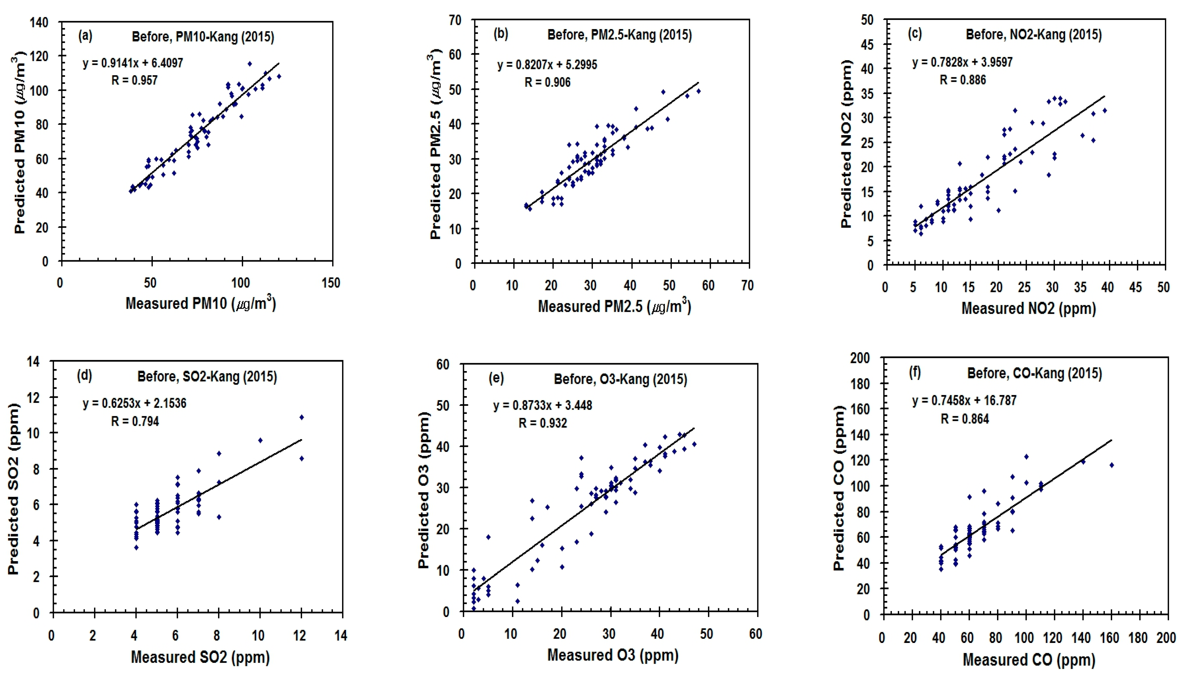
3.5. Scatter Plot and Empirical Regression Formula

Figure 6, Figure 7 and Figure 8 show scatter plots to display the comparison between the predicted and measured concentrations of PM₁₀, PM_2.5, NO₂, SO₂, O₃ and CO calculated by multivariate predictive regression models in Table 2. The scatter plots to test the goodness of the estimations of each variable present a model fitting with the calculated vs. the measured values.

The predicted values for the six hourly variables and their measured values in Figure 6 (as shown in Table 2, Table 3 and Table 4) are very highly correlated before (0.957, 0.906, 0.886, 0.795, 0.864 and 0.932), during (0.936, 0.982, 0.866, 0.917, 0.887 and 0.916) and after the yellow sand period (0.919, 0.945, 0.902, 0.857, 0.887 and 0.892), respectively. The linear regression equations in the scatter plots can also be easily used to calculate the predicted concentration of each variable from both the three-hours-earlier measured values in Kangnung and two-days-earlier measured values in Beijing.

The scatter plots to test the goodness of the estimations of each variable present a model fitting with the calculated vs. the measured values. The predicted values for the hourly PM₁₀, PM_2.5, NO₂, SO₂, O₃ and CO concentrations and their measured values in Figure 6, as shown in Table 2, are very highly correlated before (0.957, 0.906, 0.886, 0.795, 0.864 and 0.932), during (0.936, 0.982, 0.866, 0.917, 0.887 and 0.916) and after the yellow sand period (0.919, 0.945, 0.902, 0.857, 0.887 and 0.892), respectively. The linear regression equations given in the scatter plots can be easily used to calculate the predicted concentration of each variable from both the three-hours-earlier measured values in Kangnung and two-days-earlier measured values in Beijing.

Correlation coefficients between the predicted values and the measured concentrations were very high, over 0.864 for all periods, except for SO₂ (0.795, before), NO₂ (0.866, during) and SO₂ (0.857, after). These empirical regression equations to calculate the predicted values of PM₁₀, PM_2.5, NO₂, SO₂, O₃ and CO are very useful and convenient practically and can be used instead of using the multivariate regression equations in Table 2, Table 3 and Table 4 with three-hours-earlier measured values for each original PM, gas and meteorological element.

3.6. Validation of Multivariate Models

Figure 9 shows that the temporal distribution of the measured (observed) and calculated values for PM₁₀, PM_2.5, NO₂, SO₂, O₃ and CO denoted the behavior throughout each period, such as before, during and after the yellow sand periods. These figures display the real-time hourly forecasting values for PM₁₀_K(N), PM_2.5_K(N), NO₂_K(N), SO₂_K(N), O₃_K(N) and CO_K(N) calculated by multivariate regression models with the three-hours-earlier data before, during and after the yellow sand periods. Through the comparison of the predicted and measured values, we investigated in which time period the applicability of the predicted values to the measured ones was better.

Before the yellow sand period, the difference in the applicability of the real-time predicted values to the measured ones could be shown by the Pearson regression coefficients of PM₁₀_K(N) (0.957), PM_2.5_K(N) (0.906), NO₂_K(N) (0.886), O₃_K(N) (0.932) and CO_K(N) (0.864), which were slightly higher than for SO₂_K(N) (0.795). Therefore, the real-time predicted values of PM₁₀_K(N), PM_2.5_K(N), NO₂_K(N), SO₂_K(N), O₃_K(N) and CO_K(N) fit their measured values very well; even the predicted values of SO₂_K(N) were only slightly more deviated from the measured ones.

During the yellow sand event, all of the real-time predicted values fitted the measured values much better than before the event, except for NO₂_K(N), which had a slightly lower correlation coefficient. After the event, the real-time predicted values still fitted with the measured values very well and were similar to the cases before and during the yellow sand period.

As a result, the real-time predicted values of PM₁₀_K(N), PM_2.5_K(N), NO₂_K(N), SO₂_K(N), O₃_K(N) and CO_K(N) were all very close to their measured values, showing that they were reproduced well, even though the applicability of SO₂_K(N) was slightly more deviated before the yellow sand event. This means that there is a time gap between their concentrations or it has a slightly bigger or smaller value in the higher and the maximum concentrations before the period. This may be attributed to a slightly lower correlation coefficient, as shown in Figure 6 and Table 2.

We further compared our simulation results using multivariate regression models and artificial neural network models with similar scientific works by several scientists in

Table 8. Prediction performance using different models from different scientists regarding the yellow sand event (YS), with correlation coefficients (Pearson’s r). Reference: ANN-sig (Artificial neural network-sigmoid), ANN-tanh (Artificial neural network-tanh), SVM (Support vector machine), RF (Random forest), Multivariate (Multivariate regression) and SVR (Support vector regression).

Pearson r
Name	Model	Before (Hourly) YS			During (Hourly) YS			After (Hourly) YS			Daily/Seasonal/ Annual
		PM10	PM2.5	NO2	PM10	PM2.5	NO2	PM10	PM2.5	NO2	PM10	PM2.5	NO2
(1) Jeon and Son, 2018 [40]	ANN-sig										0.737
	SVM										0.751
	Random F										0.726
(2) Kim, 2019 [37]	Multivariate										0.849
(3) Lim, 2019 [38]	ANN-sig										0.962
	SVR										0.962
	Multivariate										0.958
(4) Choi and Choi, 2021 [41]	Multivariate	0.983	0.998		0.916	0.998		0.941	0.998
(5) Choi, S.-M., 2022 [39]	ANN-sig	0.954	0.866	0.873	0.941	0.960	0.975	0.930	0.953	0.917
	ANN-tanh	0.974	0.958	0.953	0.971	0.983	0.930	0.953	0.960	0.959
	Multivariate	0.961	0.909	0.896	0.948	0.977	0.875	0.920	0.947	0.903
(6) Choi et al., 2023	Multivariate	0.957	0.906	0.886	0.936	0.982	0.866	0.919	0.945	0.902

. As hourly averaged or daily averaged pollutant concentrations with or without meteorological data were used differently by individual scientists, it is not easy to compare the results calculated by each other. However, even though the same kinds of input data for the model were used, it is desirable to compare the accuracy of the different model performances.

Thus, the comparison results in Table 8 show that the correlation coefficients between the hourly predicted and measured values calculated by our multivariate regression models were 0.886 to 0.982. The accuracy of our calculated values is in the middle range compared with the results calculated using various models by other authors. If the performance of our multivariate regression model using hourly averaged input data is compared with the model performance by ANN-sig, SVR, random forest and multivariate regression using daily averaged data, it has much higher accuracy of calculation than the models performed by Jeon and Son [36] and Kim [37]; however, our model performance has relatively lower accuracy than Lim’s models. Our future research will be carried out using both artificial neural network models and multivariate regression models and the calculation results from the models will be compared with each other.

4. Conclusions

Predicting real-time air pollution concentrations in a city using historical air pollution concentration data is a very important but difficult task in all industrialized countries. The reason is that too many factors are involved and some of the air pollutants cross the border and flow into the local city, making the air pollution concentration in that city very high and the air pollution concentration also depends on the weather conditions of the city itself. In this study, we developed multivariate regression models for the real-time prediction of air quality at the current time before, during and after the yellow sand periods in Kangnung using the 3 h-earlier PM and gas concentration and meteorological parameter data from the city and the 2-days-earlier PM and gas concentration data from Beijing. Our research results are summarized as follows.

The correlation coefficient between the predicted and measured real-time PM₁₀ and PM_2.5 values calculated by the model were 0.919–0.957 and 0.906–0.945, and the prediction abilities during the event were the maximum. On the other hand, the correlation coefficients for NO₂, SO₂, O₃ and CO were 0.866–0.902, 0.795–0.917, 0.892–0.932 and 0.864–0.887, respectively, which were slightly lower than those for the PM values. However, their predicted values well reflect the measured ones and the predictive performance of our models was slightly better than other scholars’ multivariate regression models.

Before the Yellow Sand event, the PM₁₀, PM_2.5, NO₂, SO₂ and CO concentrations in Kangnung were not affected by the PM concentrations in Beijing, but some of them were affected by the gas concentrations in Beijing. During and after the yellow sand event, all PM and gas concentrations, except for O₃, in Kangnung City were affected by all PM and gas concentrations in Beijing City, except for O₃. The contribution of meteorological parameters to air pollutant concentrations in Kangnung was relatively smaller than the effect of PM and gas concentrations in Beijing City. The significance levels of all correlation coefficients were less than 0.001, indicating that they were very significant.

Generally, to predict air pollution concentrations, numerical models, multivariate regression statistical models, neural network models and meteorological satellite image interpretation methods are used. Since each method has advantages and disadvantages and the methods complement each other, I think that there is no need to analyze which method is superior. Rather, there is a need to improve each process to improve the prediction ability. Further studies of air pollution prediction in urban areas need to obtain a deeper, more comprehensive understanding the physical processes leading to the observed differences between local cities and trans-border cities for solving the nationwide air quality problem via useful models.

References

1. Gao, Y.; Anderson, J.R. Characteristics of Chinese aerosols determined by individual particle analysis. J. Geophys. Res. 2001, 106, 18037–18045. [Google Scholar] [CrossRef]
2. Lee, S.C.; Cheng, Y.; Ho, K.F.; Cao, J.J.; Loui, P.K.K.; Chow, J.C.; Watson, J.G. PM10 and PM2.5 characteristics in the roadside environment of Hong Kong. Aerosol Sci. Technol. 2006, 40, 157–165. [Google Scholar] [CrossRef]
3. Zhao, S.; Yu, Y.; Yin, D.; He, J.; Liu, N.; Qu, J.; Xiao, J. Annual and diurnal variations of gaseous and particulate pollutants in 31 provincial spatial cities based on in sit air quality monitoring data from China National Environmental Monitoring Center. Environ. Int. 2016, 86, 92–106. [Google Scholar] [CrossRef]
4. Ma, X.; Jia, H. Particulate matter and gaseous pollutions in three megacities over China: Situation and implication. Atmos. Env. 2016, 140, 476–494. [Google Scholar] [CrossRef]
5. Xiao, K.; Wang, Y.K.; Wu, G.; Fu, B.; Zhu, Y. Spatiotemporal characteristics of air pollutions (PM10, PM2.5, SO2, NO2, O3, and CO) in the inland basin city of Chengdu, Southwest China. Atmsophere 2018, 9, 74. [Google Scholar] [CrossRef]
6. Li, C.; Dai, Z.; Yang, L.; Ma, Z. Spatiotemporal characteristics of air quality across Weifang from 2014–2018. Int. J. Environ. Res. Public Health 2019, 16, 3122. [Google Scholar] [CrossRef]
7. Chow, J.C. Health effects of fine particulate air pollution; Lines that connect. J. Air Waste Manag. Assoc. 2006, 56, 707–708. [Google Scholar] [CrossRef]
8. Huang, D.; Xu, J.; Zhang, S. Valuing the health risks of particulate air pollution in the Pearl River Delta, China. Environ. Sci. Policy 2012, 15, 38–47. [Google Scholar] [CrossRef]
9. Li, F.; Liu, Y.; Lu, J.J.; Liang, L.; Harmer, P. Ambient air pollution in China poses a multi-faced health threat to outdoor physical activity. J. Epidemiol. Community Health 2015, 69, 201–204. [Google Scholar] [CrossRef]
10. Shen, F.; Ge, X.; Hu, J.; Nie, D.; Tian, L.; Chen, M. Air pollution characteristics and health risks in Henan Province, China. Environ. Res. Sci. 2017, 156, 625–634. [Google Scholar] [CrossRef]
11. He, J.Q.; Yu, X.N.; Zhu, B.; Yuan, L.; Ma, J.; Shen, L.; Zhu, J. Characteristics of aerosol extinction and low visibility in haze weather in winter of Nanjing, China. Environ. Sci. 2016, 36, 1645–1653. [Google Scholar]
12. Kim, Y.J.; Kim, K.W.; Kim, S.D.; Lee, B.K.; Han, J.S. Fine particulate matter characteristics and its impact on visibility impairment at two sites in Korea: Seoul and Incheon. Atmos. Environ. 2000, 40, 593–609. [Google Scholar] [CrossRef]
13. Sun, J.; Zhang, M.; Liu, T. Spatial and temporal characteristics of dust storms in China and its surrounding regions, 1960-1999: Relations to source area and climate. J. Geophys. Res. 2001, 10, 325–10333. [Google Scholar] [CrossRef]
14. Darmenova, K.; Sokolik, I.N.; Darmenov, A. Characterization of east Asian dust outbreaks in the spring of 2001 using ground-based and satellite data. J. Geophys. Res. 2005, 110, D02204. [Google Scholar] [CrossRef]
15. Wang, X.; Ma, Y.; Chen, H.; Wen, G.; Chen, S.; Tao, Z.; Chung, Y. The relation between sandstorms and strong winds in Xinjiang, China. Water Air Soil Pollut. Focuss 2003, 3, 67–79. [Google Scholar] [CrossRef]
16. Uno, I.; Carmichael, G.R.; Streets, D.G.; Yang, Y.; Yienger, J.J.; Satake, S.; Wang, Z.; Woo, J.H.; Guttikunda, S.; Uematsu, M.; et al. Regional chemical weather forecasting system CFORS: Model descriptions and analysis of surface observations at Japanese island stations during the ACE-Asia experiment. J. Geophys. Res. 2003, 108, 8668. [Google Scholar] [CrossRef]
17. Choi, H.; Zhang, Y.H. Predicting duststorm evolution with vorticity theory. Atmos. Res. 2008, 89, 338–350. [Google Scholar] [CrossRef]
18. Iwasaka, Y.; Shibata, T.; Nagatani, T.; Shi, G.-Y.; Kim, Y.S.; Matsuki, A.; Trochkine, D.; Zhang, D.; Yamada, M.; Nagatani, M.; et al. Large depolarization ratio of free tropospheric aerosols over the Taklamakan desert revealed by lidar measurements: Possible diffusion and transport of dust particles. J. Geophys. Res. 2003, 108, 8652. [Google Scholar] [CrossRef]
19. Gao, T.; Su, L.; Ma, Q.; Li, H.; Yu, X. Climate analyses on increasing dust storm frequency in the springs of 2000 and 2001 in Inner Mongolia. Int. J. Climatol. 2003, 23, 1743–1755. [Google Scholar] [CrossRef]
20. Sun, J. Provenance of loess material and formation of deposits on the Chinese Loess Plateau. Earth Planet. Sci. Lett. 2002, 203, 845–859. [Google Scholar] [CrossRef]
21. Chung, Y.S.; Kim, H.S.; Natsagdorj, L.; Jugder, D.; Chen, S.J. On yellow sand occurred during 1997–2000. J. Korean Meteor. Soc. 2001, 37, 305–316. [Google Scholar] [CrossRef]
22. Zhang, X.Y.; Gong, S.L.; Shen, Z.X.; Mei, F.M.; Xi, X.X.; Liu, L.C.; Zhou, Z.J.; Wang, D.; Wang, Y.Q.; Cheng, Y. Characteristics of soil dust, aerosol in China an its transport and distribution during 2001 ACE-Asia: 1: Network observations. J. Geophys. Res. 2003, 108, 4261. [Google Scholar] [CrossRef]
23. He, Z.; Kim, Y.J.; Ogunjobi, O.; Hong, C.S. Characteristics of PM2.5 species and long-range transport of air masses at Taeanback ground station, South Korea. Atmos. Environ. 2003, 37, 219–230. [Google Scholar] [CrossRef]
24. Kim, K.W.; Kim, Y.J.; Oh, S.J. Visibility impairment during Yellow Sand periods in the urban atmosphere of Kwangju, Korea. Atmos. Environ. 2001, 35, 5157–5167. [Google Scholar] [CrossRef]
25. Shim, K.; Kim, M.-H.; Lee, H.-J.; Nishizawa, T.; Shimizu, A.; Kobayashi, H.; Kim, C.-H.; Kim, S.-W. Exacerbation of PM2.5 concentration due to unpredictable weak Asian dust storm: A case study of an extraordinarily long-lasting spring haze episode in Seoul, Korea. Atmos. Environ. 2022, 287, 119261. [Google Scholar] [CrossRef]
26. Lin, T.H. Long-range transport of yellow sand to Taiwan in spring 2000: Observed evidence and simulation. Atmos. Environ. 2001, 35, 5873–5882. [Google Scholar] [CrossRef]
27. Uno, I.; Amano, H.; Emori, S.; Kinoshita, K.; Matsui, I.; Sugimoto, N. Tans-Pacific yellow sand transport observed in April, 1998: A numerical simulation. J. Geophys. Res. 2001, 106, 18331–18344. [Google Scholar] [CrossRef]
28. Chin, M.; Ginoux, P.; Lucchesi, R.; Huebert, B.; Weber, R.; Anderson, T.; Masonis, S.; Blomquist, B.; Bandy, A.; Thomton, D. A global aerosol model forecast for the ACE-Asia field experiment. J. Geophys. Res. 2003, 108, 8654. [Google Scholar] [CrossRef]
29. Jaffe, D.; McKendry, I.; Anderson, T.; Price, H. Six "new" episodes of trans-Pacific transport of air pollutants. Atmos. Environ. 2003, 37, 391–404. [Google Scholar] [CrossRef]
30. McKendry, I.G.; Hacker, J.P.; Stull, R.; Sakiyama, S.; Mignacca, D.; Reid, K. Long-range transport of Asian dust to the lower Fraser Valley, British Columbia, Canada. J. Geophys. Res. 2001, 106, 18361–18370. [Google Scholar] [CrossRef]
31. Lee, M.S.; Chung, J.D. Impact of yellow dust transport from Gobi Desert on fractional ratio and correlations of temporal PM10, PM2.5 and PM1 at Gangneung city. J. Environ. Sci. 2012, 21, 217–231. [Google Scholar] [CrossRef]
32. Bhaskar, B.V.; Mehta, V.M. Atmospheric particulate pollutants and their relationship with meteorology in Ahmedabad. Aerosol. Air Qual. Res. 2010, 10, 301–315. [Google Scholar] [CrossRef]
33. Cheng, Y.; He, K.B.; Du, Z.Y.; Zheng, M.; Duan, F.K.; Ma, Y.L. Humidity plays an important role in the PM2.5 pollution in Beijing. Environ. Pollut. 2015, 197, 68–75. [Google Scholar] [CrossRef] [PubMed]
34. Li, X.; Ma, Y.; Wang, Y.; Liu, N.; Hong, Y. Temporal and spatial analysis of particulate matter (PM10 and PM2.5) and its relationship with meteorological parameters over an urban city in northeast China, 2017. Atmos. Res. 2017, 198, 185–193. [Google Scholar] [CrossRef]
35. Shi, C.; Yuan, R.; Wu, B.; Meng, Y.; Zhang, H.; Zhang, H.; Gong, Z. Meteorological conditions to PM2.5 pollution in winter 2016/2017 in the western Yangtze delta, China. Sci. Total Environ. 2018, 642, 1221–1232. [Google Scholar] [CrossRef]
36. Zhao, D.; Chen, H.; Yu, E.; Luo, T. PM2.5/PM10 ratios in eight economic regions and their relationship with meteorology in China. Adv. Meteorol. 2019, 5295726. [Google Scholar] [CrossRef]
37. Kim, M.J. The effects of transboundary air pollution from China on ambient air quality in South Korea. Heliyon 2019, 5, e06283. [Google Scholar] [CrossRef]
38. Lim, J.-M. An estimation model of fine dust concentration using meteorological environment data and machine learning. J. Inform. Technol. 2019, 18, 173–185. [Google Scholar]
39. Choi, S.-M. Implementation of Prediction System on Urban Air Quality Using Artificial Neural Network and Multivariate Regression Models during the COVID-19 Pandemic and Yellow Dust Event. Ph.D. Thesis, Konkuk University, Seoul, Republic of Korea; pp. 1–268.
40. Jeon, S.; Son, Y.S. Prediction of fine dust PM10 using a deep neural network model. Korean J. Appl. Stat. 2018, 31, 205–285. [Google Scholar]
41. Choi, S.-M.; Choi, H. Statistical modeling for PM10, PM2.5, and PM1 at Gangneung affected by local meteorological variables and PM10 and PM2.5 at Beijing for non- and dust periods. App. Sci. 2021, 11, 11958. [Google Scholar] [CrossRef]
42. Mendez, M.R.; Souto, J.A.; Vila-Guerau de Arellano, J.; Lucas, T.; Casares, J.J. Dispersion and transformation of nitrogen oxides emitted from a point source. WIT Trans. Ecol. Environ. 1997, 19, 10. [Google Scholar]
43. Chu, B.; Zhang, S.; Liu, J.; Ma, Q.; He, H. Significant concurrent decrease in PM2.5 and NO2 concentrations in China during COVID-19 epidemic. J. Environ. Sci. 2021, 99, 346–353. [Google Scholar] [CrossRef] [PubMed]
Figure 1. Geographical map of northeastern Asia with the Gobi Desert in southern Mongolia (big square) and Beijing (China; red star) and Kangnung (Korea; red circle) cities.
Applsci 13 10556 g001
Figure 2. GONE-2 (METOP-B) KNMI/O3MSAF/EUMETSAT satellite images reflecting a cloud of dust on (a) 19 March 2015 (before) and (b) 22 March (during the period of the yellow sand event in Korea). Small blue squares and circles denote Beijing (China) and Kangnung (Korea). (https://www.temis.nl/aviation/aai-archive.php?Year=2015&Month=03&Day=19, accessed on 25 February 2023).
Applsci 13 10556 g002
Figure 3. Hourly distribution of (a) PM10 and PM2.5 concentrations (μg/m3) and (b) SO2 (×1000), (c) CO (×100), (d) O3 (×1000) and NO2 (×1000) concentrations (ppm) before, during and after the yellow sand period at the Okcheondong observation point in Kangnung city (Korea), corresponding to the PM concentrations on 16 to 25 March at the Yongdingmen observation point in Beijing city (China).
Applsci 13 10556 g003
Figure 4. Hourly distributions of (a) air temperature (°C; TEMP), (b) wind speed (m/s; WIND) and (c) relative humidity (%; RH) at Kangnung in Korea (modified from [41]).
Applsci 13 10556 g004aApplsci 13 10556 g004b
Figure 5. Hourly distribution of (a) PM10 and PM2.5 concentrations (μg/m3) and (b) SO2 (×1000), (c) CO (×100), (d) O3 (×1000) and NO2 (×1000) concentrations (ppm) at the Yongdingmen observation point in Beijing (China), corresponding to PM concentrations on 18 to 27 March at Kangnung, Korea.
Applsci 13 10556 g005
Figure 6. Scatter plots between the measured and predicted concentrations of PM10 (a), PM2.5 (b) (μg/m3) and NO2 (×1000) (c), SO2 (×1000) (d), O3 (×1000) (e), and CO (×100) (f) (ppm) before the yellow sand event from 21 March to 21 March 2015 in Kangnung, Korea.
Applsci 13 10556 g006
Figure 7. As Figure 6, but for during the event from 21 March to 23 March 2015. PM10 (a), PM2.5 (b) (μg/m3) and NO2 (×1000) (c), SO2 (×1000) (d), O3 (×1000) (e), and CO (×100) (f) (ppm).
Applsci 13 10556 g007
Figure 8. As Figure 6, but for after the event from 23 March to 27 March 2015. PM10 (a), PM2.5 (b) (μg/m3) and NO2 (×1000) (c), SO2 (×1000) (d), O3 (×1000) (e), and CO (×100) (f) (ppm).
Applsci 13 10556 g008
Figure 9. Temporal variations of the measured and real-time predicted values of PM10 (a), PM2.5 (b) ( μ g/m3) and NO2 (×1000) (c), SO2 (×1000) (d), O3 (×1000) (e) and CO (×100) (f) (ppm) in Kangnung, Korea.
Applsci 13 10556 g009aApplsci 13 10556 g009b