A Data Analytic Monitoring with IoT System of the Reproductive Conditions of the Red Worm as a Product Diversification Strategy

Abstract

The Internet of Things (IoT) is becoming increasingly important due to the ability to collect data in real time and monitor the performance of systems. In this sense, the objective of the project is to create an IoT system to monitor and enhance red boll worm farming conditions in California as part of a strategy to diversify annelid-based goods. Therefore, the goal is to expand this animal’s productivity so that additional items can be made from California red worms. Furthermore, the method used implies a research design that uses an experimental approach to obtain data based on the variable conditions identified in the literature review. The analysis of the data will allow determination of the factors that result in optimization of production, and at the same time creation of a production estimation in the network platform. Finally, this project proposes to facilitate the monitoring and control of the variables that interfere in the earthworm reproduction process to increase the production of annelids in pursuit of product diversification. In addition, we put it into practice in real life to demonstrate its applicability and efficacy. In this mode, the results indicate potential findings about IoT application in agriculture situations.

1. Introduction

The Californian red worm has been examined in many regions of the world because it is a species with a high concentration of nutrients and a high reproductive rate when compared to other types of worms [1,2,3]. Numerous studies have been conducted to determine the various kinds of worms used in worm farming [4,5], and it appears that the California red worm is the best species for this kind of activity [6,7,8]. Worm farming is an activity which has been engaged in for 50 years in the United States, and it is also a very significant activity in Mexico [9]. In addition, many of the studies that were looked at show how the worm behaves in various temperatures and levels of humidity, but few record how the pH behaves, and a wide variety of studies looked at the possibility of improving the conditions for reproduction under various types of nutrition [10].

In the department of Norte de Santander, there are some associated production units that are dedicated to vermiculture and that present the need to increase production to cover the departmental demand and open national and international markets. Starting from an evaluation of opportunities to improve the farms, the need arises to identify optimal conditions to ensure that the Californian red worm reproduces in greater quantities over time under the current conditions of the city, which would allow the consideration of new ventures and greater competitiveness.

Numerous studies focusing on applications, experimentation, and research in the realm of applied sciences have also been conducted [11,12,13]. Similarly, technological development today is one of the greatest sources of wealth for nations, as long as it is applied to the service of solutions to social, economic, and environmental problems [14,15,16]. In addition, the Internet of Things (IoT) represents a potential system to collect information in agriculture situations in real time [17,18,19,20,21]. In this sense, the IoT system continuously monitors and maintains the necessary parameters at optimal levels, reducing the need for human involvement in the process of vermicomposting [22].

According to the literature review, there are three gaps that need to be addressed:

• Currently, the worm beds are automated for irrigation and temperature measurement; however, variables such as humidity and feeding have not been taken into account, and these study variables are referenced in the literature [23].
• The feeding of the worms is carried out without any control [24].
• Different foods are supplied from food residues mixed with bovine excrement, without recording dietary measurements.

The motivation of this work is to find a model that is able to take into consideration data obtained directly from system sensors for vermiculture production based on the estimated model, and at the same time handle statistical information. In this regard, the contributions provided in this paper are listed as follows:

• Identify through the literature review the levels of factors that affect the reproduction of the Californian red worm.
• Analyze the effect of the factors (Humidity, Temperature, pH, and Type of food) and their levels on the reproduction of the Californian red worm.
• Create a monitoring system for vermiculture production based on an IoT system. Figure 1 depicts the graphical user interface of the system.
• Finally, provide a validation of the monitoring system via statistical and comparative study using the TODIM method.

2. Methodology

In this section, the methodology proposed is presented. Figure 2 depicts the flowchart explaining the steps of the methodology used.

Step 1: Ethical considerations: In accordance with Resolution 008430 of 1993—article 11 of the Ministry of Health, the risks of an investigation are classified as: without risk, minimal risk and high risk. This research is classified among the projects without risk, because it does not work on the human being, nor is any intentional intervention or modification made to the biological, physiological, psychological or social variables of the individuals participating in the study.

In accordance with article 87 of this same resolution, it is specified that the animals that will be taken into account for this project will not suffer physical alterations nor will their bodies be intervened with to obtain information. An observation will be made on variables such as temperature which are not lethal and do not cause episodes of distress to the animal.

Under Russel and Burch’s 3R principle, this research uses the reduction alternatives that refer to any strategy that results in the use of a smaller number of animals to obtain sufficient data to answer the question investigated, which in this case is the maximization of reproduction, in order to potentially limit or prevent further use by other animals without compromising animal welfare. Taking into account Law 84 of 1989, this project does not cause harm to an animal nor does it contemplate behaviors considered cruel to the worms under study, nor will animal sacrifice actions be carried out since their behavior is only observed in their natural state.

Step 2: Determine the variable of control of the experiment. In this mode, the experimental units, responses and variables need to be identified.

The experimental unit is the Californian red worm and the response variable is the weight of the beds in kg. The generic diagram of the experiment can be seen in Figure 3.

In this mode, the mathematical expression can be documented in Equation (1).

$$Y_z=x_1·y_1+x_2·y_2+x_3·y_3$$

(1)

where

1.

$Y_z$: Represents the solutions obtained from the calculations, where an optimal solution is desired.

2.

$x_1$: Corresponds to the humidity factor.

3.

$x_2$: Belongs to the temperature factor of the system.

4.

$x_3$: Represents the time factor.

5.

$y_1$: Describes the equipment used to build the system.

6.

$y_2$: Represents the environmental conditions.

7.

$y_3$: Depicts the circle of life beds of the system.

Step 3: Establish a design of experiments.

The application of factorial design of experiments is used to find the best levels of the variables. The operator of the association’s worm beds will be in charge of taking the data at the times established by the work team. During data collection, the basic principles of the design of experiments will be guaranteed as follows:

• Randomization: With the help of the R software 4.3.1, the order in which the configuration of the factor levels is assigned among the 36 beds is obtained, which is done randomly. This will guarantee the independence of the observations.
• Replication: According to the data in the problem statement, factor $x_1$ has three levels, as well as factors $x_2$, and $x_3$, which results in the calculation of the total number of observations shown in Equation (2), where n is the number of replicas which is four; in this experiment, it is possible to find an experimental error for each sample and the sources of variability are found in each replica taken by combination. This ensures replication as a principle.

  $$N=3^3·n=27·4=108$$

  (2)
• Blocking: To guarantee the blocking principle, certain aspects must be taken into account. For example, the species of the worms must be the same (California red); it is important to maintain the same supplier of worms and supplier of food for each type selected; water that is supplied to the beds must be obtained from the same place; and the use of the same supplier of the measurement equipment installed in each bed must be guaranteed.

Step 4: Implement the system of automation and control of variables:

Within the framework of the field visit to the farm where the automation of the prototype of the irrigation system is carried out to control the temperature and humidity variables of vermiculture, the electronic and communications system was implemented through the TTGO programmable card for real-time monitoring of the system.

After making adjustments, the system is implemented in the vermiculture and the corresponding electrical connections are established for the connection of automated irrigation and the reading of the variables. In this mode, the following Figure 4 shows the installation of the system:

Finally, the Internet connection of the TTGO programmable card is verified to receive the data through the advances generated in the development of the web platform, such as system plan images. The sensor is installed 10 cm from the ground or soil where the worms are. The sensor is a DTH22 type with a −40 °C to 80 °C temperature range and a 0.5 °C precision. It has a precision of 2% RH and a humidity range of 0 to 100% RH. Therefore, the influence or impact of weather on the measurements is not taken into account. The sensor is also placed 10 cm from the test ground. The experiment location has a roof and is surrounded by trees, providing protection from rain and solar radiation. 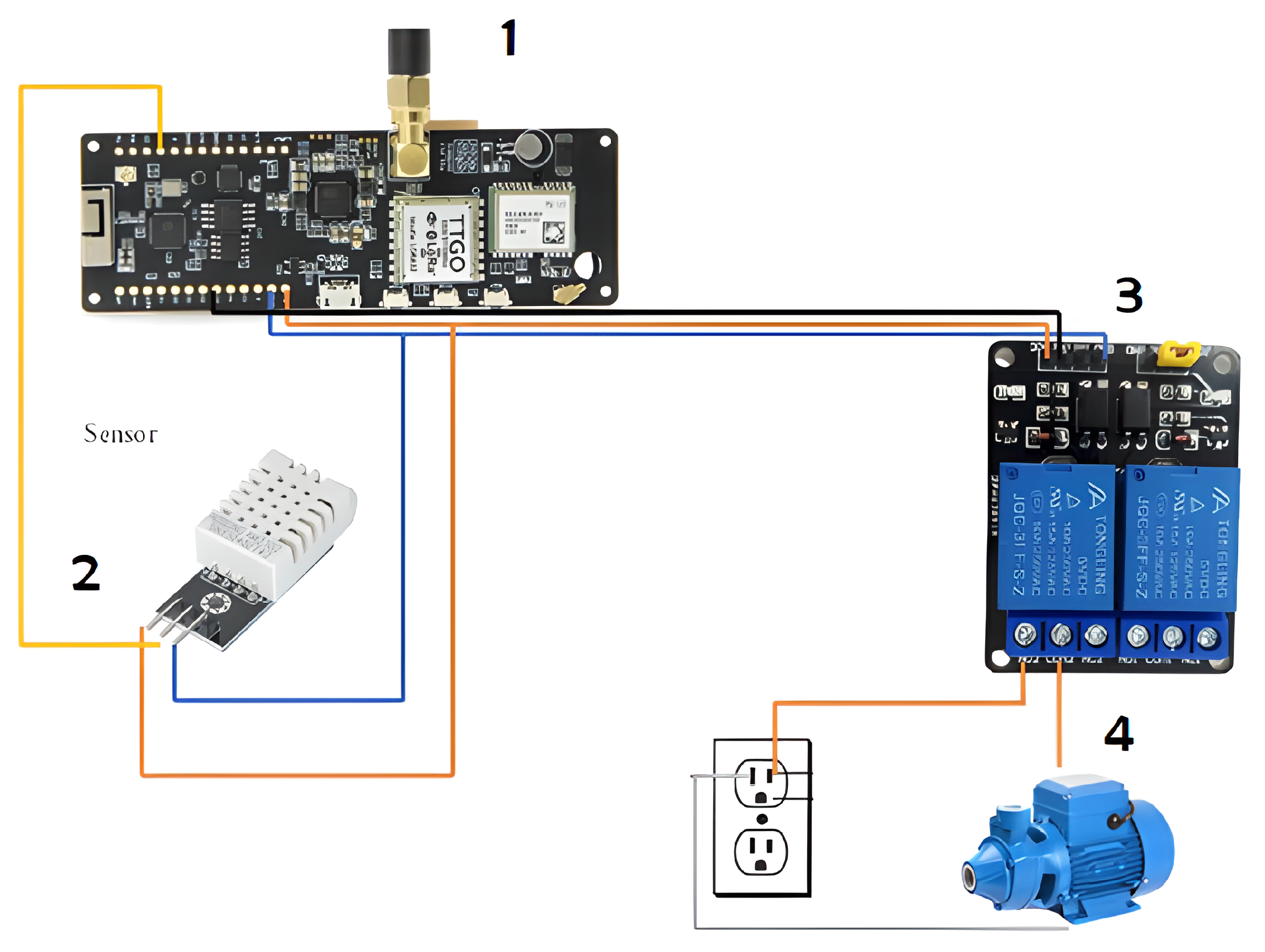Figure 5 depicts the diagram of the system connection.

In this mode, the explanation in detail is presented as follows:

1.

The TTGO development board is the main controller and communication system of the system because it contains various modules. It is responsible for reading the signals from the sensors to activate or deactivate the actuators, according to the rules defined by the user through the ESP32 module. Likewise, it is in charge of making the Internet connection through the Wi-Fi module, to send the data on temperature, humidity and status of the actuators, updating the information every 5 min in the cloud; the information is visible on the web through the platform ubidots on smartphones or computers. It is powered by a 3.7 to 4.2 VDC battery.

2.

The DTH22 sensor allows monitoring of temperature and relative humidity; it works with levels from 3 to 6 VDC, which allows the use of the 5 VDC power pins of the TTGO card. It can measure temperatures between −40 and 80 °C and humidity from 0 to 100%. The information about the measured variables is delivered digitally, so a communication interface with the TTGO card is not necessary.

3.

The two-channel relay module is used to activate the irrigation pump. It connects with the TTGO card to receive the activation control signals and power through its VCC GND, and signal terminals. It has the function of making the connection between the control stage of the TTGO card and the power stage of the water pump, since it has opto-couplers that allow the protection of the card from power voltages and handle loads with a maximum current of 10 A and up to 250 VAC.

4.

The water pump works as the actuator of the system to provide humidity; it works with AC current, and its power is half a horsepower. It is controlled from the TTGO card through the two-channel relay module.

5.

The temperature and humidity data that are measured with the DTH22 sensor are sent by Wi-Fi communication using the TTGO card. Programming with the Arduino interface is used for the tasks of communication, storage and visualization of the data. For Wi-Fi communication, the ESP32 module and the internal Wi-Fi module are programmed on the TTGO card. Likewise, through Arduino libraries, the Ubidots IoT software is used where the sensor data are stored and displayed through the Ubidots user interface on computers or smartphones.

6.

The DHT22 sensor has an accuracy of 0.5 °C, which allows for very accurate temperature readings, unlike commercial sensors such as the DHT11 that have an accuracy of 2 °C. On the other hand, the TTGO card has several modules to be used in different functions, such as ESP32, LORA communication, WI-FI. It incorporates GPS and multiple inputs and outputs to work with analog and digital signals, and a battery power supply; this allows the card to be deployed in any rural environment and to use the most convenient communication. The technologies that merge in this research are IoT and agriculture, since telecommunications, electronics and agriculture sciences are used to improve humus production.

7.

The water was sprayed in the form of a mist using plastic nebulizer sprinklers so that the moisture stayed on the surface and the worms were always at the top, eating the food and depositing the fertilizer at the bottom. If any errors are discovered, the watchdog will reset the system.

The recording of the data in reading the variables in real time through a mobile device is evidenced. Figure 6 depicts the project, which is developed with seven worm beds; each bed has an area of 24 m${}^2$ (2 m wide × 12 m long).

Figure 6 depicts how cow excrement is used as worm food. After wetting and drying the manure, it is allowed to rest for two to three weeks so that the gastric acids from the cattle can be removed before the worms use it as food. Worms typically consume 250 kg of food per month, but once the system was installed, this amount climbed to an average of 650 kg per month, which shortened the time it took to produce humus or compost.

Step 5: Defining the path of data analysis:

Construct the instrument to collect the information. For data collection, temperature and humidity sensors and weight scales will be implemented. The measurements will be carried out by the same operator daily and will be recorded in a technical sheet designed by the authors.

For the analysis of the data collected, it is intended to execute the following route, depicted in Figure 7, which is aligned with the objectives of the project and allows the expected results to be obtained:

3. Analysis and Discussion of Results

In the bibliographic review, it was found that the factors identified by the vermiculturists have been studied separately. Many studies focus on three of them: temperature, humidity and feeding. The pH was found to be an important factor, but there are no studies that deepen knowledge of this aspect; in the same way, there was no evidence of studies where the interactions of the factors are analyzed.

In

Table 1. Identification of factors that affect the reproduction of the Californian red worm.

Authors	Studied Factor
	Humidity	Temperature	pH	Type of Food
Toccalino et al. [25]	X	X		X
Durán and Henríquez [26]	X	X		X
Domínguez and Gómez-Brandón [27]	X	X
Feijoo et al. [28]			X
Domínguez et al. [29]				X
Fragoso [9]				X
Paco et al. [30]	X	X	X
Murguía et al. [23]	X	X	X	X
Toccalino et al. [31]	X	X	X	X
Rodríguez [32]	X	X	X	X
Vázquez et al. [33]	X	X	X	X
García et al. [34]				X
Rodríguez-Dimas et al. [35]	X

, you can see the review of some studies and a summary of the main factors studied because they affect in some way the mortality rate of earthworms or their reproduction.

3.1. Identification of Factor Levels

The review of the literature allowed us to identify the factors that influence the mortality rate and the reproduction process of the Californian red worm. It also allows us to estimate some values of the levels of each factor.

Table 2. Identification of levels worked in different studies for each factor.

Authors	Studied Factor
	Humidity	Temperature	pH
Toccalino et al. [25]	80%	19 °C	Does not register
Durán and Henríquez [26]	70–80%	15–25 °C	Does not register
Domínguez and Gómez-Brandón [27]	80–85%	25 °C	Does not register
Feijoo et al. [28]	Does not register	Does not register	4.4–7.2
Domínguez et al. [29]	Does not register	Does not register	Does not register
Fragoso [9]	Does not register	Does not register	Does not register
Paco et al. [30]	77–89%	17–22 °C	7.17–8.2
Loza Murguía et al. [23]	75%	17–22 °C	7–7.58
Toccalino et al. [31]	80%	18.1–20.4 °C	6.31–6.88
Rodríguez-Dimas et al. [35]	80%	10–25 °C	7.09–8.17
Vázquez et al. [33]	80%	24–26 °C	The pH does not affect
García et al. [34]	Does not register	Does not register	Does not register

shows the working values of each factor (humidity and temperature) for each article reviewed.

The feeding factor in each of the articles varies; each experiment used different diets and concluded if they were satisfactory or not.

Table 3. Feeding of the Californian red worm according to the bibliographic review.

Authors	Worm Feeding
Toccalino et al. [25]	The reproduction of earthworms in treated beds with compost from bovine manure produced the highest values of offspring (expressed in number of pups at 14 and 21 days and for the total number of pups per ootheca).
Durán and Henríquez [26]	It was found that treatments with lower average weight were those that produced a larger number of capsules (manure, ornamental and brush).
Domínguez and Gómez-Brandón [27]	The most mentioned are litter, feces and decomposing organic matter (does not analyze which is the best).
Domínguez et al. [29]	Some feed mainly on microbes (microbivores), other matter decomposing organic (detritivores), others from a mixture of organic matter and microbes (microbi-detritivores), however; no comparison is made of feeding.
Loza Murguía et al. [23]	The relation of the weight of the population of worms in bovine dung is shown; it is observed that its weight gradually decreases as the density increases. This indicates that the food is a condition for the weight of the individual to be affected.
Toccalino et al. [31]	The production in captivity of earthworms fed with bovine manure originates a more prolific ootheca, since they originate a greater number of pups per ootheca.
Rodríguez-Dimas et al. [35]	It was detected that the cow is the best for the reproduction of worms with an average of 17,471 per m3 and a ratio of 50:1. It is recommended to use the cow and pulp of coffee for the reproduction of the worm as well as for quick production of biofertilizer.
Vázquez et al. [33]	In the composted bovine manure were found the greatest number of cocoons (201.75 ± 94.46) and young earthworms (3.25 ± 2.50), and the highest viability of worm adults (45.25 ± 15.19), compared to composted sheep manure which presented a lower number of cocoons (89.0 ± 11.74) and did not present any young worms; however, it had greater viability of adult worms (81.75 ± 16.47). The results indicated that composted manures are the best in terms of earthworm population dynamics, compared to fresh manures.

shows the different feeding options found.

In summary,

Table 4. Levels chosen for each factor and their convention.

Convention	Humidity	Temperature	Food
Low; 0	70%	15 °C	Composting from bovine manure
Medium; 1	80%	20 °C	Vacaza and coffee pulp
High; 2	89%	25 °C	Composted sheep manure

defines the levels to be evaluated in the experiment taking into account the results presented in each study of the bibliographic review, the experience of the animalist of the association of worm farmers and the repetition of these values.

3.2. Analysis and Discussion of Results

The analysis below will be performed taking into account the factors that were used for the design of the experiment.

Table 5. Averages Replica 1.

Humidity	Temperature	Diet
		Coffee	Ovine	Bovine
70	15	4920.1
70	20	4911.1
70	25			5078.2
80	15	5296
80	20			5475.3
80	25		5342
89	15			5110.1
89	20		5283
89	25	4903.1

depicts a summary of the main factors. These are: Humidity: this factor contains three levels which are 70, 80 and 89. Temperature: this factor contains three levels which are 15, 20 and 25. Diet: this is a categorical type factor which has three levels: coffee, sheep and bovine averages.

To start, the averages are graphed and the sum of the differences in the mean of the treatments with the global mean is established. In this manner,

Table 6. Global Averages.

Humidity	Temperature	Diet
		Coffee	Ovine	Bovine
70	15	4956.6
70	20	4967.5
70	25			5588.8
80	15	5610.5
80	20			5854.9
80	25		5739.2
89	15			5263.2
89	20		5343.1
89	25	5406.6

shows the global averages of the treatments.

3.2.1. Diet Factor

Let i be the iteration element between the levels of the $\alpha$ (diet factor), then we have that the difference of the averages of the grouped treatments that include each type of diet is obtained with Equation (3):

$$\alpha ={\overline{Y}}_{i\dots }-{\overline{Y}}_{\dots .}$$

(3)

In addition, when performing an analysis of the averages and the sum of the difference of squares with the mean, it is observed that the replicas have different levels of results in their relationship with the weight variable, being the “sheep” and “bovine” diets the ones that present a higher average, observing, the sum of squares of the difference with the global average of the data allows identifying important effects, this is visible in the result of the effect of the averages of the diet when comparing it with the global average. Figure 8 depicts the averages of the grouped treatments.

3.2.2. Moisture Factor

Let j be the iteration element between the levels of the “humidity” factor; then, we obtain that the difference of the averages of the grouped treatments that include each type of humidity is computed using Equation (4), where $\beta$ corresponds to the humidity factor obtained with treatments generated.

$$\beta ={\overline{Y}}_{j\dots }-{\overline{Y}}_{.\dots }$$

(4)

An overview of the treatment averages is presented in Figure 9.

The sums of squares with respect to the global mean for diet are contained in

Table 7. Squared difference from global mean.

	Coffee	Ovine	Bovine	SCDiet
1	19,312.7	27,551.4	5570.5	629,215.7
R2	59,276.2	3998.9	44,192.7	1,289,613.3
R1 + R2	26,194.1	19,162.2	14,718.2	1,501,861.6

. In this mode, $R1$ and $R2$ are squared differences with the overall mean for the diet types.

The sum of squares measurements of variations or deviations from the general mean for temperature (T) are shown in

Table 8. Squared difference with the overall mean.

	T = 15	T = 20	T = 25	SCTemperature
R1	1430.5	5864.2	1502	105,560
R2	68,487.8	23,298.3	117,029.3	2,505,785.1
R1 + R2	12,342	2423.5	26,503.4	1,031,723.8

. Likewise, $R1$ and $R2$ are squared differences with the overall mean related to the temperature levels.

Interaction between factors: Diet ∼ Moisture Interaction

This is defined as the interaction component between “diet” i and “moisture” j “Sheep” diet factor—humidity.

Figure 10 allows us to infer that the level of the temperature factor that registers the greater weight of the bedding is 20 °C.

Thus, regarding the humidity factor, it can also be seen in Figure 11 that time affects the weight of the beds because the longer the time, the higher the value of the response variable, and it can be seen that the level with the highest value of the response variable is 80% when 28 days have elapsed.

3.3. Comparative Study with Multi-Criteria Using the TODIM Method

The TODIM (an abbreviation for Interactive and Multi-Criteria Decision Making in Portuguese) application is based on a multi-criteria global value function proposed by Gomes and Lima (1991) [36]. The TODIM method depicts a prominent tool to appraisal MCDM problem situation [37]. In fact, this mathematic function is built in parts, with their mathematical descriptions reproducing the profit/loss function of prospect theory. The multi-attribute global value function then aggregates all win and loss measures across all criteria.

Step 1: As a first step for the implementation of TODIM, the corresponding decision matrix must be exposed.

Table 9. Decision matrix.

Item	Levels	Humidity	Temperature	Coffee	Ovine	Bovine
N1	Low	70	15	4920.1	0	0
N2	Low-Medium	70	20	4911.1	0	0
N3	Low-High	70	25	0	0	5078.2
N4	Medium-Low	80	15	5296	0	0
N5	Medium-Medium	80	20	0	0	5475.3
N6	Medium-High	80	25	0	5342	0
N7	High-Low	89	15	0	0	5110.1
N8	High-Medium	89	20	0	5283	0
N9	High-High	89	25	4903.1	0	0

describes the decision matrix to be with the variable to be analyzed.

Step 2: To make this decision matrix dimensionless and all its elements comparable, we normalize.

Table 10. Normalized Matrix.

Levels	C1	C2	C3	C4	C5
N1	0.098	0.083	0.246	0.000	0.000
N2	0.098	0.111	0.245	0.000	0.000
N3	0.098	0.139	0.000	0.000	0.324
N4	0.112	0.083	0.264	0.000	0.000
N5	0.112	0.111	0.000	0.000	0.350
N6	0.112	0.139	0.000	0.503	0.000
N7	0.124	0.083	0.000	0.000	0.326
N8	0.124	0.111	0.000	0.497	0.000
N9	0.124	0.139	0.245	0.000	0.000

depicts the normalized decision matrix to capture the weighted information.

Step 3: Determine the degree of dominance of alternative $A_i$ over alternative $A_j$.

Table 11. Dominance degree for alternative $A1$ in regard to each criterion.

Levels	C1	C2	C3	C4	C5	$⋋({\mathit{A}}_{\mathit{i}},{\mathit{A}}_{\mathit{j}})$
N2	0.000	−0.333	0.007	0.000	0.000	−0.326
N3	0.000	−0.471	0.172	0.000	−2.013	−2.313
N4	−0.165	0.000	−0.395	0.000	0.000	−0.561
N5	−0.165	−0.333	0.172	0.000	−2.090	−2.417
N6	−0.165	−0.471	0.172	−3.545	0.000	−4.010
N7	−0.228	0.000	0.172	0.000	−2.019	−2.076
N8	−0.228	−0.333	0.172	−3.526	0.000	−3.915
N9	−0.228	−0.471	0.010	0.000	0.000	−0.689

presents the dominance matrix of the alternative $A1$ where the weight vectors $w=[0.510.250.120.040.08]$ which were computed using the AHP approach will be used for the case study.

Table 12. Dominance degree for alternative $A2$ in regard to each criterion.

Levels	C1	C2	C3	C4	C5	$⋋({\mathit{A}}_{\mathit{i}},{\mathit{A}}_{\mathit{j}})$
N1	0.000	0.000	0.000	0.000	0.000	0.000
N3	0.000	−0.333	0.172	0.000	−2.013	−2.175
N4	−0.165	0.083	−0.400	0.000	0.000	−0.482
N5	−0.165	0.000	0.172	0.000	−2.090	−2.084
N6	−0.165	−0.333	0.172	−3.545	0.000	−3.873
N7	−0.228	0.083	0.172	0.000	−2.019	−1.992
N8	−0.228	0.000	0.172	−3.526	0.000	−3.582
N9	−0.228	−0.333	0.007	0.000	0.000	−0.554

presents the dominance matrix of the alternative $A2$.

Table 13. Dominance degree for alternative $A3$ in regard to each criterion.

Levels	C1	C2	C3	C4	C5	$⋋({\mathit{A}}_{\mathit{i}},{\mathit{A}}_{\mathit{j}})$
N1	0.000	0.083	−1.429	0.000	0.161	−1.185
N2	0.000	0.000	0.000	0.000	0.000	0.000
N4	−0.165	0.118	−1.484	0.000	0.161	−1.371
N5	−0.165	0.083	0.000	0.000	−0.563	−0.645
N6	−0.165	0.000	0.000	−3.545	0.161	−3.550
N7	−0.228	0.118	0.000	0.000	−0.160	−0.270
N8	−0.228	0.083	0.000	−3.526	0.161	−3.509
N9	−0.228	0.000	−1.428	0.000	0.161	−1.495

presents the dominance matrix of the alternative $A3$.

Table 14. Dominance degree for alternative $A4$ in regard to each criterion.

Levels	C1	C2	C3	C4	C5	$⋋({\mathit{A}}_{\mathit{i}},{\mathit{A}}_{\mathit{j}})$
N1	0.084	−0.333	0.048	0.000	0.000	−0.201
N2	0.084	−0.471	0.178	0.000	−2.013	−2.222
N3	0.000	0.000	0.000	0.000	0.000	0.000
N5	0.000	−0.333	0.178	0.000	−2.090	−2.246
N6	0.000	−0.471	0.178	−3.545	0.000	−3.839
N7	−0.157	0.000	0.178	0.000	−2.019	−1.998
N8	−0.157	−0.333	0.178	−3.526	0.000	−3.838
N9	−0.157	−0.471	0.049	0.000	0.000	−0.580

presents the dominance matrix of the alternative $A4$.

Table 15. Dominance degree for alternative $A5$ in regard to each criterion.

Levels	C1	C2	C3	C4	C5	$⋋({\mathit{A}}_{\mathit{i}},{\mathit{A}}_{\mathit{j}})$
N1	0.084	0.000	−1.429	0.000	0.167	−1.178
N2	0.084	−0.333	0.000	0.000	0.045	−0.204
N3	0.000	0.083	−1.484	0.000	0.167	−1.234
N4	0.000	0.000	0.000	0.000	0.000	0.000
N6	0.000	−0.333	0.000	−3.545	0.167	−3.711
N7	−0.157	0.083	0.000	0.000	0.043	-0.030
N8	−0.157	0.000	0.000	−3.526	0.167	−3.515
N9	−0.157	−0.333	−1.428	0.000	0.167	−1.751

presents the dominance matrix of the alternative $A5$.

Table 16. Dominance degree for alternative $A6$ in regard to each criterion.

Levels	C1	C2	C3	C4	C5	$⋋({\mathit{A}}_{\mathit{i}},{\mathit{A}}_{\mathit{j}})$
N1	0.084	0.083	−1.429	0.142	0.000	−1.120
N2	0.084	0.000	0.000	0.142	−2.013	−1.787
N3	0.000	0.118	−1.484	0.142	0.000	−1.225
N4	0.000	0.083	0.000	0.142	−2.090	−1.865
N5	0.000	0.000	0.000	0.000	0.000	0.000
N7	−0.157	0.118	0.000	0.142	−2.019	−1.917
N8	−0.157	0.083	0.000	0.015	0.000	−0.059
N9	−0.157	0.000	−1.428	0.142	0.000	−1.443

presents the dominance matrix of the alternative $A6$.

Table 17. Dominance degree for alternative $A7$ in regard to each criterion.

Levels	C1	C2	C3	C4	C5	$⋋({\mathit{A}}_{\mathit{i}},{\mathit{A}}_{\mathit{j}})$
N1	0.116	−0.333	−1.429	0.000	0.162	−1.485
N2	0.116	−0.471	0.000	0.000	0.013	−0.342
N3	0.080	0.000	−1.484	0.000	0.162	−1.243
N4	0.080	−0.333	0.000	0.000	−0.540	−0.793
N5	0.080	−0.471	0.000	−3.545	0.162	−3.775
N6	0.000	0.000	0.000	0.000	0.000	0.000
N8	0.000	−0.333	0.000	−3.526	0.162	−3.697
N9	0.000	−0.471	−1.428	0.000	0.162	−1.738

presents the dominance matrix of the alternative $A7$.

Table 18. Dominance degree for alternative $A8$ in regard to each criterion.

Levels	C1	C2	C3	C4	C5	$⋋({\mathit{A}}_{\mathit{i}},{\mathit{A}}_{\mathit{j}})$
N1	0.116	0.000	−1.429	0.141	0.000	−1.172
N2	0.116	−0.333	0.000	0.141	−2.013	−2.089
N3	0.080	0.083	−1.484	0.141	0.000	−1.180
N4	0.080	0.000	0.000	0.141	−2.090	−1.869
N5	0.080	−0.333	0.000	−0.373	0.000	−0.626
N6	0.000	0.083	0.000	0.141	−2.019	−1.795
N7	0.000	0.000	0.000	0.000	0.000	0.000
N9	0.000	−0.333	−1.428	0.141	0.000	−1.621

presents the dominance matrix of the alternative $A8$.

Finally,

Table 19. Dominance degree for alternative $A9$ in regard to each criterion.

Levels	C1	C2	C3	C4	C5	$⋋({\mathit{A}}_{\mathit{i}},{\mathit{A}}_{\mathit{j}})$
N1	0.116	0.083	−0.058	0.000	0.000	0.142
N2	0.116	0.000	0.171	0.000	−2.013	−1.725
N3	0.080	0.118	−0.404	0.000	0.000	−0.206
N4	0.080	0.083	0.171	0.000	−2.090	−1.756
N5	0.080	0.000	0.171	−3.545	0.000	−3.294
N6	0.000	0.118	0.171	0.000	−2.019	−1.730
N7	0.000	0.083	0.171	−3.526	0.000	−3.271
N8	0.000	0.000	0.000	0.000	0.000	0.000

presents the dominance matrix of the alternative $A9$.

Step 4: The degree of general dominance of the alternative is determined by applying the corresponding equation.

Table 20. Levels’ overall dominance degrees.

Levels	$\sum ⋋({\mathit{A}}_{\mathit{i}},{\mathit{A}}_{\mathit{j}})$	${\mathit{\varsigma }}_{\mathit{i}}$
N1	−16.308	0.000
N2	−14.743	0.227
N3	−12.025	0.621
N4	−14.923	0.201
N5	−11.624	0.680
N6	−9.415	1.000
N7	−13.074	0.469
N8	−10.352	0.864
N9	−11.841	0.648

presents the overall dominance degrees of the alternatives (levels).

Step 5: Finally, the alternatives are ranked in descending order of their dominance scores and the alternative with the highest dominance score obviously becomes the best option.

Table 21. Ranking of the levels based on ${\varsigma }_i$ values.

Levels	${\mathit{\varsigma }}_{\mathit{i}}$	Ranking
N1	0.000	9
N2	0.227	7
N3	0.621	5
N4	0.201	8
N5	0.680	3
N6	1.000	1
N7	0.469	6
N8	0.864	2
N9	0.648	4

describes the rankings of the alternatives.

Figure 12 depicts that level N6 denoted in yellow color corresponds to the combination of levels of humidity of 80 and temperature of 25.

Level N6 is equivalent to the optimal decision-making, as shown in Figure 13.

Finally, the validations of the results are consistent to confirm that level $N6$ depicts the best solution. The findings obtained with the TODIM method and the statistical tests are significant to validate the results.

4. Conclusions

This research has an exploratory scope with an experimental approach because the state of the worm is not altered to obtain data and the variables are observed as they are generated to validate a model in real time; it has the endorsement of one of the vermiculture companies in the department of Norte de Santander, who lent some beds for the measurement of the variables. The scope is descriptive with the use of quantitative theories for the mathematical modeling of the system. It is intended to describe the optimal state of the observable variables to maximize the production of the Californian red worm.

In real experiments, variables that cannot be controlled but that directly affect the process pH must be taken into account because they must be measured and analyzed in order to generate true conclusions regarding the phenomenon under study. Please note that in our study, only the parameters of temperature, humidity and diet were considered. Monitoring the pH was omitted; in future works, it will be taken into account.

The experiment can be designed with a Box–Behnken approach, taking into account experimental conditions that are not possible to execute in the reality of the process, since this DOE excludes combinations where all factor levels are high and all are low. For this case, the low temperature level (15 °C) was difficult to control, mainly influenced by the ambient temperature (35 °C). Additionally, the design of experiments (DOE) analysis and the TODIM technique validation both significantly reported the same levels.

Finally, we consider that our findings are robust enough to provide a solution to this kind of problem. Additionally, the IoT represents a potential support to monitoring the reproductive conditions of the red worm. In future works, it can be applied to diverse MCDM methods to compare the scenarios and explore which economic factors are involved in the manufacturing process.

References

1. Lavelle, P. Earthworm activities and the soil system. Biol. Fertil. Soils 1988, 6, 237–251. [Google Scholar] [CrossRef]
2. Wang, Z.; An, Y.; Chen, H.; Zhang, J.; Zhang, H.; Zhu, G.; Chen, J.; Li, W.; Wang, J.; Xu, H.J.; et al. Effects of Earthworms and Phosphate-Solubilizing Bacteria on Carbon Sequestration in Soils Amended with Manure and Slurry: A 4-Year Field Study. Agronomy 2022, 12, 2064. [Google Scholar] [CrossRef]
3. Arnone, J.A.; Zaller, J.G.; Hofer, G.; Schmid, B.; Körner, C. Loss of plant biodiversity eliminates stimulatory effect of elevated CO2 on earthworm activity in grasslands. Oecologia 2013, 171, 613–622. [Google Scholar] [CrossRef] [PubMed]
4. Arancon, N.; Edwards, C.; Bierman, P.; Welch, C.; Metzger, J. Influences of vermicomposts on field strawberries: 1. Effects on growth and yields. Bioresour. Technol. 2004, 93, 145–153. [Google Scholar] [CrossRef]
5. Ning, Y.; Wang, X.; Lu, J.; Li, Y.; Yang, Y.; Zou, D.; Zhou, D. Study on the life maintenance mechanism of Eisenia fetida under low-density polyethylene stress: Based on path analysis and canonical correlation analysis. Ecotoxicol. Environ. Saf. 2023, 250, 114500. [Google Scholar] [CrossRef]
6. Edwards, C.A.; Arancon, N.Q. The Role of Earthworms in Organic matter and nutrient cycles. In Biology and Ecology of Earthworms; Springer: New York, NY, USA, 2022; pp. 233–274. [Google Scholar]
7. Jun-Zhu, P.; Yu-Hui, Q.; Zhen-Jun, S.; Zhang, S.X.; Yun-Le, L.; Zhang, R.Q. Effects of epigeic earthworms on decomposition of wheat straw and nutrient cycling in agricultural soils in a reclaimed salinity area: A microcosm study. Pedosphere 2012, 22, 726–735. [Google Scholar]
8. Ansari, A.; Wrights, J.; Jaikishun, S. Earthworms in Bioremediation of Soils Contaminated with Petroleum Hydrocarbons. In Vermicomposting for Sustainable Food Systems in Africa; Springer: Berlin/Heidelberg, Germany, 2023; pp. 349–368. [Google Scholar]
9. Fragoso, C. Las lombrices de tierra de México (Annelida, Oligochaeta): Diversidad, ecología y manejo. Acta Zool. Mex. 2001, Es-1, 131–171. [Google Scholar] [CrossRef]
10. Edwards, C.A.; Arancon, N.Q. Earthworm Life Histories and Biology. In Biology and Ecology of Earthworms; Springer: Berlin/Heidelberg, Germany, 2022; pp. 81–108. [Google Scholar]
11. Quy, V.K.; Hau, N.V.; Anh, D.V.; Quy, N.M.; Ban, N.T.; Lanza, S.; Randazzo, G.; Muzirafuti, A. IoT-enabled smart agriculture: Architecture, applications, and challenges. Appl. Sci. 2022, 12, 3396. [Google Scholar] [CrossRef]
12. Tam, P.; Corrado, R.; Eang, C.; Kim, S. Applicability of Deep Reinforcement Learning for Efficient Federated Learning in Massive IoT Communications. Appl. Sci. 2023, 13, 3083. [Google Scholar] [CrossRef]
13. Contreras-Castillo, J.; Guerrero-Ibañez, J.A.; Santana-Mancilla, P.C.; Anido-Rifón, L. SAgric-IoT: An IoT-Based Platform and Deep Learning for Greenhouse Monitoring. Appl. Sci. 2023, 13, 1961. [Google Scholar] [CrossRef]
14. Lebrouhi, B.; Djoupo, J.; Lamrani, B.; Benabdelaziz, K.; Kousksou, T. Global hydrogen development—A technological and geopolitical overview. Int. J. Hydrogen Energy 2022, 47, 7016–7048. [Google Scholar] [CrossRef]
15. Pham, H.S.T.; Nguyen, A.N.; Johnston, A. Economic policies and technological development of Vietnaḿs electronics industry. J. Asia Pac. Econ. 2022, 27, 248–269. [Google Scholar] [CrossRef]
16. Navarro, E.; Costa, N.; Pereira, A. A systematic review of IoT solutions for smart farming. Sensors 2020, 20, 4231. [Google Scholar] [CrossRef] [PubMed]
17. Čolaković, A.; Hadžialić, M. Internet of Things (IoT): A review of enabling technologies, challenges, and open research issues. Comput. Netw. 2018, 144, 17–39. [Google Scholar] [CrossRef]
18. Rukhiran, M.; Netinant, P. IoT Architecture based on Information Flow Diagram for Vermiculture Smart Farming Kit. TEM J. 2020, 9, 1330. [Google Scholar] [CrossRef]
19. Zou, X.; Liu, W.; Huo, Z.; Wang, S.; Chen, Z.; Xin, C.; Bai, Y.; Liang, Z.; Gong, Y.; Qian, Y.; et al. Current Status and Prospects of Research on Sensor Fault Diagnosis of Agricultural Internet of Things. Sensors 2023, 23, 2528. [Google Scholar] [CrossRef]
20. Bulut, C.; Wu, P.F. More than two decades of research on IoT in agriculture: A systematic literature review. Internet Res. 2023. ahead-of-print. [Google Scholar] [CrossRef]
21. Pathmudi, V.R.; Khatri, N.; Kumar, S.; Abdul-Qawy, A.S.H.; Vyas, A.K. A systematic review of IoT technologies and their constituents for smart and sustainable agriculture applications. Sci. Afr. 2023, 19, e01577. [Google Scholar] [CrossRef]
22. Bagali, V.; Jiddi, V.; Jahagirdar, W. Vermicomposting of Biodegrable Waste: An Iot based Approach. In Proceedings of the 2021 5th International Conference on Electrical, Electronics, Communication, Computer Technologies and Optimization Techniques (ICEECCOT), Mysuru, India, 10–11 December 2021; IEEE: New York, NY, USA, 2021; pp. 443–447. [Google Scholar]
23. Murguía, M.L.; Mamani, B.C.; Tancara, H.P.; Tintaya, D.H.; Osorio, I.C.; Palero, B.C. Comportamiento de lombriz roja californiana y lombriz silvestre en bosta bovina y rumia bovina como sustrato. Rev. Mex. Cienc. Agrícol. 2010, 1, 555–565. [Google Scholar]
24. Anderson, G.L.; Boyd, W.A.; Williams, P.L. Assessment of sublethal endpoints for toxicity testing with the nematode Caenorhabditis elegans. Environ. Toxicol. Chem. Int. J. 2001, 20, 833–838. [Google Scholar] [CrossRef]
25. Toccalino, P.; Agüero, M.; Serebrinsky, C.; Roux, J.P. Comportamiento reproductivo de lombriz roja californiana (Eisenia foetida) según estación del año y tipo de alimentación. Rev. Vet. 2004, 15, 65–69. [Google Scholar]
26. Durán, L.; Henríquez, C. Crecimiento y reproducción de la lombriz roja (Eisenia foetida) en cinco sustratos orgánicos. Agron. Costarric. 2009, 33, 275–281. [Google Scholar]
27. Domínguez, J.; Gómez-Brandón, M. Ciclos de vida de las lombrices de tierra aptas para el vermicompostaje. Acta Zool. Mex. 2010, 26, 309–320. [Google Scholar] [CrossRef]
28. Feijoo, A.; Quintero, H.; Fragoso, C.; Moreno, A.G. Patrón de distribución y listado de especies de las lombrices de tierra (Annelida, Oligochaeta) en Colombia. Acta Zool. Mex. 2004, 20, 197–220. [Google Scholar] [CrossRef]
29. Domínguez, J.; Aira, M.; Gómez-Brandón, M. El papel de las lombrices de tierra en la descomposición de la materia orgánica y el ciclo de nutrientes. Ecosistemas 2009, 18, 20–31. Available online: https://www.revistaecosistemas.net/index.php/ecosistemas/article/view/61 (accessed on 25 October 2022).
30. Paco, G.; Loza-Murguía, M.; Mamani, F.; Sainz, H. Efecto de la Lombriz Roja Californiana (Eisenia fetida) durante el composteo y vermicomposteo en predios de la Estación Experimental de la Unidad Académica Campesina Carmen Pampa. J. Selva Andin. Res. Soc. 2011, 2, 24–39. [Google Scholar]
31. Toccalino, P.A.; Roux, J.P.; Agüero, C.M. Comportamiento reproductivo de Eisenia foetida (lombriz roja de California) durante las cuatro estaciones del año y alimentadas con distintos compostajes. Univ. Nac. Nord. Fac. Cien. Vet. 2001, 40, 1–3. Available online: http://www.bio-nica.info/biblioteca/toccalino1999.pdf (accessed on 16 November 2022).
32. Rodríguez, Á.R. Producción y Calidad de Abono Orgánico por Medio de la Lombriz Roja Californiana (Eisenia foetida) y Su Capacidad Reproductiva; Informe Técnico; Instituto Hondureño del Café (IHCAFE): Tegucigalpa, Honduras, 1996. [Google Scholar]
33. Vázquez, E.G.; Caratachea, A.J.; Mondragón, A.J.; Sandoval, A.L.R. Dinámica poblacional de la lombriz Eisenia fetida en estiércol composteado y fresco de bovino y ovino. Redvet. Rev. Electrón. Vet. 2007, 8, 1–8. [Google Scholar]
34. García, M.; Espinosa, M.G.N.; López, C.N.V.; López, J.V. Elaboración de abono orgánico a base de lombriz roja californiana. Estud. Agrar. 2013. Available online: https://biblat.unam.mx/es/revista/estudios-agrarios/articulo/elaboracion-de-abono-organico-a-base-de-lombriz-roja-californiana (accessed on 5 December 2022).
35. Rodríguez-Dimas, N.; Cano-Ríos, P.; Figueroa-Viramontes, U.; Palomo-Gil, A.; Favela-Chávez, E.; de Paul Álvarez-Reyna, V.; Márquez-Hernández, C.; Moreno-Reséndez, A. Producción de tomate en invernadero con humus de lombriz como sustrato. Rev. Fitotec. Mex. 2008, 31, 265–272. [Google Scholar] [CrossRef]
36. Gomes, L.; Lima, M. TODIMI: Basics and application to multicriteria ranking. Found. Comput. Decis. Sci 1991, 16, 1–16. [Google Scholar]
37. Tian, X.; Li, W.; Liu, L.; Kou, G. Development of TODIM with different types of fuzzy sets: A state-of the-art survey. Appl. Soft Comput. 2021, 111, 107661. [Google Scholar] [CrossRef]
Figure 1. The graphical user interface of the system.
Applsci 13 10522 g001
Figure 2. Sequence of methodology.
Applsci 13 10522 g002
Figure 3. General scheme of the design of the Californian earthworm experiment.
Applsci 13 10522 g003
Figure 4. Installation and protection of the system control box.
Applsci 13 10522 g004
Figure 5. Diagram of the system implemented in the worm crop.
Applsci 13 10522 g005
Figure 6. Test of the automated irrigation system for the control of the humidity and temperature variables.
Applsci 13 10522 g006
Figure 7. Analysis Route.
Applsci 13 10522 g007
Figure 8. Averages of the grouped treatments.
Applsci 13 10522 g008
Figure 9. Treatment averages.
Applsci 13 10522 g009
Figure 10. Effect of time towards the response variable of the temperature factor.
Applsci 13 10522 g010
Figure 11. Effect of time towards the response variable of the humidity factor.
Applsci 13 10522 g011
Figure 12. Dominance scores.
Applsci 13 10522 g012
Figure 13. Spider chart indicating levels.
Applsci 13 10522 g013