Enhancing Density Prediction of Agricultural Land Soil through Void Area Curve Analysis

Abstract

Thresholding is a digital image analysis method used to distinguish objects from the background in images and it is mainly used for void and density analysis in soil. It is important to select an appropriate thresholding method because the accuracy of void analysis can vary significantly depending on the threshold value; however, there is currently no standard for soil density analysis. Therefore, this study proposes an image analysis method for soil density prediction. The experimental process involved collecting soil samples from agricultural lands, encompassing various soil textures including sandy loam, loam, silt loam, and silty clay loam. These samples were then meticulously prepared under controlled conditions, ensuring a comprehensive range of dry densities and water content levels. Digital images of the soil samples were acquired using a Canon EOS100d camera, employing a high-resolution setup that provided precise imaging capabilities. The porosity of the soil image is calculated by various thresholding methods. Based on the analysis results, we propose a void area curve, a new approach that can be applied to the soil density prediction. The void area curve is the relationship curve between the threshold value and porosity of the soil image. The standard deviation of the void area curve showed a high correlation with the dry density of the soil. The standard deviation of the void area curve was used to predict the dry density under various soil texture and water content conditions, and the RMSE was 0.037 t/m³. The method of estimating soil density with the standard deviation of the void area curve can be used more generally than the existing analysis method because there is no need to select a specific threshold value.

1. Introduction

In agricultural land, the soil density is a factor that greatly affects crop growth [1,2,3]. Soil density also greatly influences the pore size, water infiltration, and aeration, which greatly affects the crop growth [4,5]. The soil density is obtained through in situ density tests such as the sand cone method, drive cylinder method, and nuclear method [6]. All of these methods provide reliable data; however, they are difficult to use in agricultural lands where numerous tests are required. The soil density in agricultural land continuously changes with tillage and agricultural management; as a result, it is necessary to develop a method that can quickly identify soil densities at various points [7,8]. Therefore, a new method for density management in agricultural lands is needed.

Soil pores are classified into macropores, mesopores, micropores, ultramicropores, and cryptopores according to their size, with macropores larger than 0.075 mm being highly dependent on soil density [9,10,11]. Accordingly, it is possible to predict soil density by observing changes in soil macropores.

Digital image processing (DIP) is receiving great attention as a methodology to replace the existing experimental method. DIP is a process of extracting desired data through the appropriate processing of images [12]. DIP enables low cost, rapid, quantitative, versatile, and nondestructive analysis [13,14,15,16,17,18]. As an extension of visual observation, DIP is widely used in various fields, such as medicine, aviation, and manufacturing, and is also used to analyze soil characteristics [19,20,21]. Examples of soil analysis using DIP include soil constituents [19], soil redoximorphic features [20], particle size distribution [21,22], void distribution analysis [23], crack analysis [15,24], and tensile strength [25]. X-ray microtomography creates a three-dimensional, precise image of the inside of a sample with a resolution better than 1 micrometer, enabling noninvasive analysis of the composition and pore space of the sample [26,27]. However, such detailed analysis techniques are still expensive for application in the agricultural field. The performance of digital cameras has significantly developed recently. The soil density prediction using commercial level digital cameras will be of great help to agricultural land soil management. For this purpose, Kim et al. [28,29] performed an image analysis of soil density using a commercial-level digital camera with a deep neural network and reported an RMSE of 0.044 to 0.107 t/m³ using a convolutional neural network and an RMSE of 0.080 t/m³ using a deep neural network.

Visible-near-infrared (vis-NIR) spectroscopy stands out as a rapid and nondestructive technique, demonstrating its ability to predict soil properties both in laboratory and field settings, as highlighted by studies conducted by Yang et al. [30] and Davari et al. [31]. Vis-NIR spectroscopy is commonly incorporated with traditional calibration methods such as partial least squares regression (PLSR), support vector machines regression (SVMR), random forests (RF), or, more recently, neural network techniques to improve accuracy [30]. Furthermore, vis-NIR spectroscopy has found utility in predicting soil density. Researchers have achieved this by combining it with gamma-ray attenuation, as demonstrated by Lobsey and Rossel [32], or by employing PLSR algorithms, as evidenced by the investigations of Xu et al. [33] and Katuwal et al. [34]. In their study, Lobsey and Rossel [32] successfully calibrated measurements from a gamma-ray attenuation sensor alongside vis-NIR data to predict bulk density, achieving a result with a root mean square error of only 0.055 g/cm³. Similarly, Xu et al. [33] reported a moderate R² value of 0.63 for bulk density prediction by employing vis-NIR in conjunction with PLSR. Meanwhile, Katuwal et al. [34] demonstrated bulk density prediction within the range of 1.02 to 2.01 g/cm³, achieving an R² value of 0.46. Despite its cost and time effectiveness [31,35], vis-NIR spectroscopy does pose a challenge due to its reliance on specialized equipment, a limitation that mirrors the constraints associated with X-ray microtomography, thus impeding its widespread adoption in general agricultural fields.

What is necessary for soil density analysis by digital images is to separate voids and soil areas, and thresholding can be used for this purpose. Thresholding is an image processing method mainly used to distinguish between an object and a background in an image [36]. In a soil image, the soil solids are the objects and the voids are the background. Abd El-Halim [24] and Peng et al. [15] quantified and analyzed soil cracks by performing thresholding on soil images. Bruneau et al. [14] and Passoni et al. [37] also performed thresholding to analyze the void distribution. Each researcher applied the automatic thresholding method provided by the image processing software or, if necessary, determined the threshold value based on the pixel intensity distribution curve and performed the analysis. The most important factor in thresholding is to determine the threshold value. There are various methods for thresholding; however, there is no standard related to soil analysis [38]. Since there is no standard for thresholding methods for soil analysis, the accuracy of the soil density analysis may vary depending on the selection of the thresholding method. Therefore, it is necessary to determine which of the various thresholding methods is suitable for soil density analysis, or to propose an image analysis method suitable for density analysis.

Therefore, this study aims to investigate thresholding methods suitable for soil image-based density estimation using common digital cameras. For this purpose, soils from agricultural fields were prepared under various water content and dry density conditions and digital images were acquired. The digital images of the soil underwent thresholding using the results of simple thresholding at different threshold values and representative automatic thresholding methods such as the Otsu method and Triangle method. Through the analysis of the threshold images, the limitations of the existing thresholding methods in predicting soil density were analyzed, and based on this, a new analysis method suitable for predicting soil density, the void area curve method, was proposed. The void area curve method is a new analysis method that can overcome the limitations of the existing analysis methods, whose accuracy may vary depending on the selection of the threshold value, and can be widely used for soil density analysis.

2. Materials and Methods

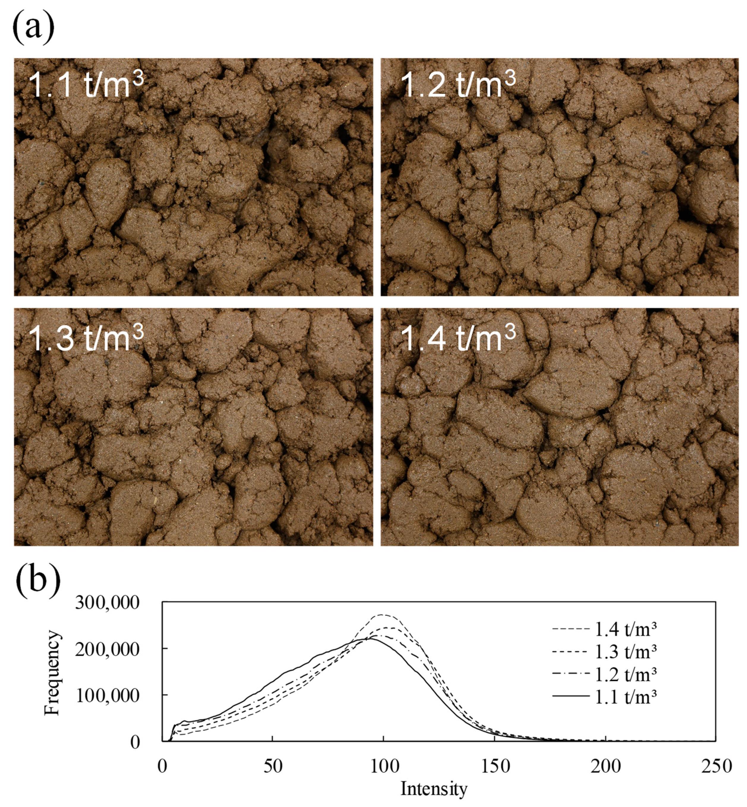
2.1. Image Acquisition for Soil Samples

The soil samples used in this study were collected from agricultural lands. The condition of the soil samples for image analysis is summarized in

Table 1. Condition of the soil samples for image analysis.

Soil Sample Condition			Repetition	Total Images
Texture	Dry Density (t/m3)	Water Content (%)
SL, L, SiL, SiCL	1.1, 1.2, 1.3, 1.4	5, 10, 15, 20, 25	3 times	240

. Soil samples were classified as sandy loam (SL), loam (L), silt loam (SiL), and silty clay loam (SiCL) by the USDA soil classification methods. From SL towards L and SiL, the content of sand gradually decreases and the content of silt increases. SiCL is a soil with a lower content of silt and a higher content of clay compared to SiL. Each soil was oven-dried at 110 ± 5 °C for 24 h and then water was added to adjust the water content to 5, 10, 15, 20, and 25%. The wet soil was then compacted into cylindrical acrylic molds to prepare samples for image acquisition. The size of the mold was 150 mm in diameter and 50 mm in height. The dry density of the soil in the mold was adjusted to 1.1, 1.2, 1.3, and 1.4 t/m³. The ranges of dry density and water content were determined in consideration of general field soil conditions. Each soil sample was prepared in triplicate under the same conditions. Therefore, the total number of samples was 240, 60 for each soil. A Canon EOS100d camera (Canon Inc., Tokyo, Japan) was installed in the vertical direction of the soil sample. The size of the image was 5184 horizontal pixels and 3456 vertical pixels, and the resolution was 0.018 mm/pixel. Digital images were acquired under a controlled constant light condition.

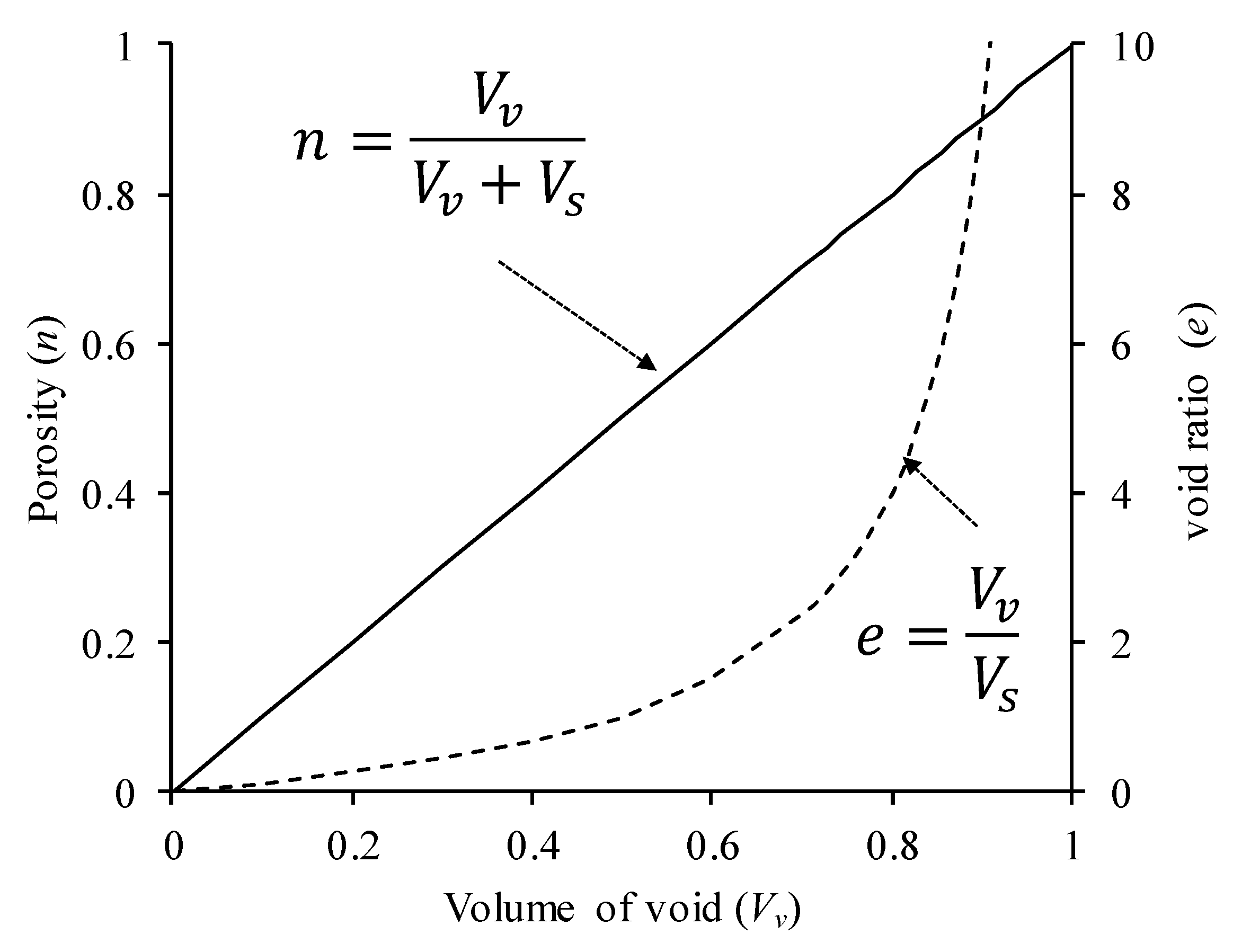
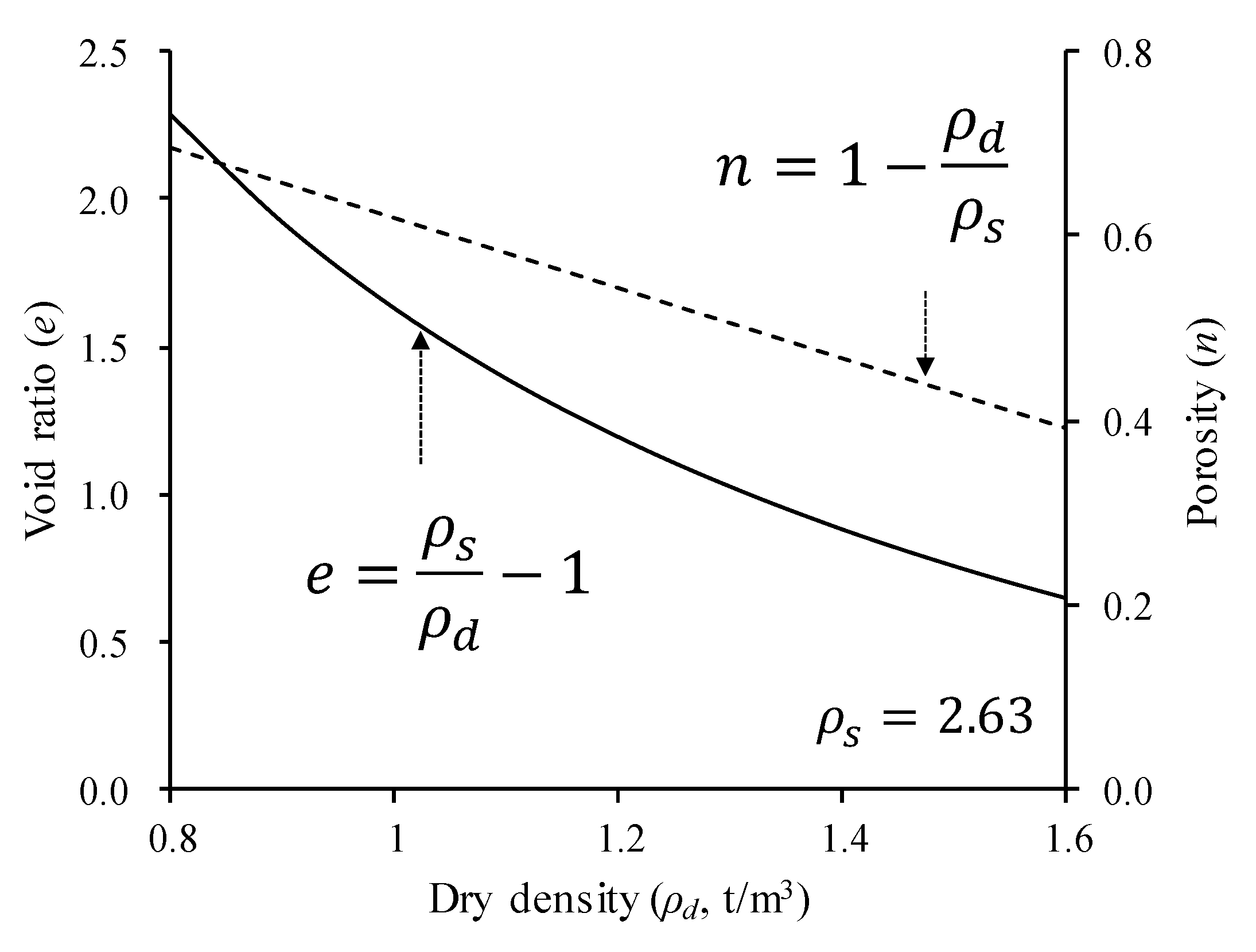
2.2. Void Area in the Soil Image

Soil mass comprises three phases: solids (soil particles), water, and air. The composition of the volume of the soil mass is shown in Equation (1) [39].

$$V_t=V_s+V_w+V_a=V_s+V_v$$

(1)

where $V_t$ is the total volume, $V_s$ is the volume of the solids, $V_w$ is the volume of the water, $V_a$ is the volume of the air, and $V_v$ is the volume of the void. The dry density of the soil is defined as the ratio of the total volume of soil ($V_t$) to the mass of soil particles ($W_s$) and represents the degree of compaction. When the soil is compacted, the dry density increases because the void and total volume of the soil decreases. Therefore, if the void of the soil can be quantified, the dry density can be predicted. The voids in the soil can be quantified as the void ratio ($e$) or porosity ($n$), which are expressed by Equations (2) and (3), respectively [39].

$$e=V_v/V_s=V_v/(V_t-V_v)=n/(1-n)$$

(2)

$$n=V_v/V_t=V_v/(V_v+V_s)=e/(1+e)$$

(3)

$V_t$ is a constant of the sum of $V_s$ and $V_v$. Figure 1 shows the change in $e$ and $n$ according to $V_v$ when $V_t$ is 1.

As $V_v$ increases, both $e$ and $n$ tend to increase. $n$ increases linearly with $V_v$, ranging from a minimum of 0 to a maximum of 1. $e$ increases exponentially with respect to $V_v$ and diverges as $V_v$ approaches 1. Equations (2) and (3) can be rewritten by the specific gravity of the soil (${\rho }_s$) and dry density (${\rho }_d$) as Equations (4) and (5).

$$e=\frac{n}{1-n}=\frac{1-\frac{{\rho }_d}{{\rho }_s}}{1-(1-\frac{{\rho }_d}{{\rho }_s})}=\frac{\frac{{\rho }_s-{\rho }_d}{{\rho }_s}}{\frac{{\rho }_d}{{\rho }_s}}=\frac{{\rho }_s-{\rho }_d}{{\rho }_d}=\frac{{\rho }_s}{{\rho }_d}-1$$

(4)

$$n=\frac{V_v}{V_t}=\frac{V_t-V_s}{V_t}=1-\frac{V_s}{V_t}=1-\frac{W_s{V}_s}{V_t{W}_s}=1-\frac{{\rho }_d}{{\rho }_s}$$

(5)

The changes of $e$ and $n$ according to ${\rho }_d$ are shown in Figure 2.

$n$ is linearly proportional to ${\rho }_d$ and $V_v$. Therefore, if $n$ can be quantified using soil $V_v$, ${\rho }_d$ can be predicted. However, because the volume cannot be obtained from a two-dimensional soil image, $n$ must be calculated indirectly through an area rather than a volume [40]. The porosity in the digital image ($n^{\prime }$) based on the area of the void in the digital image rather than the volume is expressed in Equation (6).

$$n^{\prime }=A_v/A_t$$

(6)

$n^{\prime }$ is the porosity in the digital image, $A_v$ is the area of the void in the digital image, and $A_t$ is the total area of the digital image. The basic unit of area in a digital image is the pixel. Accordingly, Equation (6) can be rewritten as Equation (7).

$$n^{\prime }=A_v/A_t=N_{void}/N_{total}$$

(7)

where $N_{void}$ is the number of pixels of the void and $N_{total}$ is the total number of pixels in the digital image.

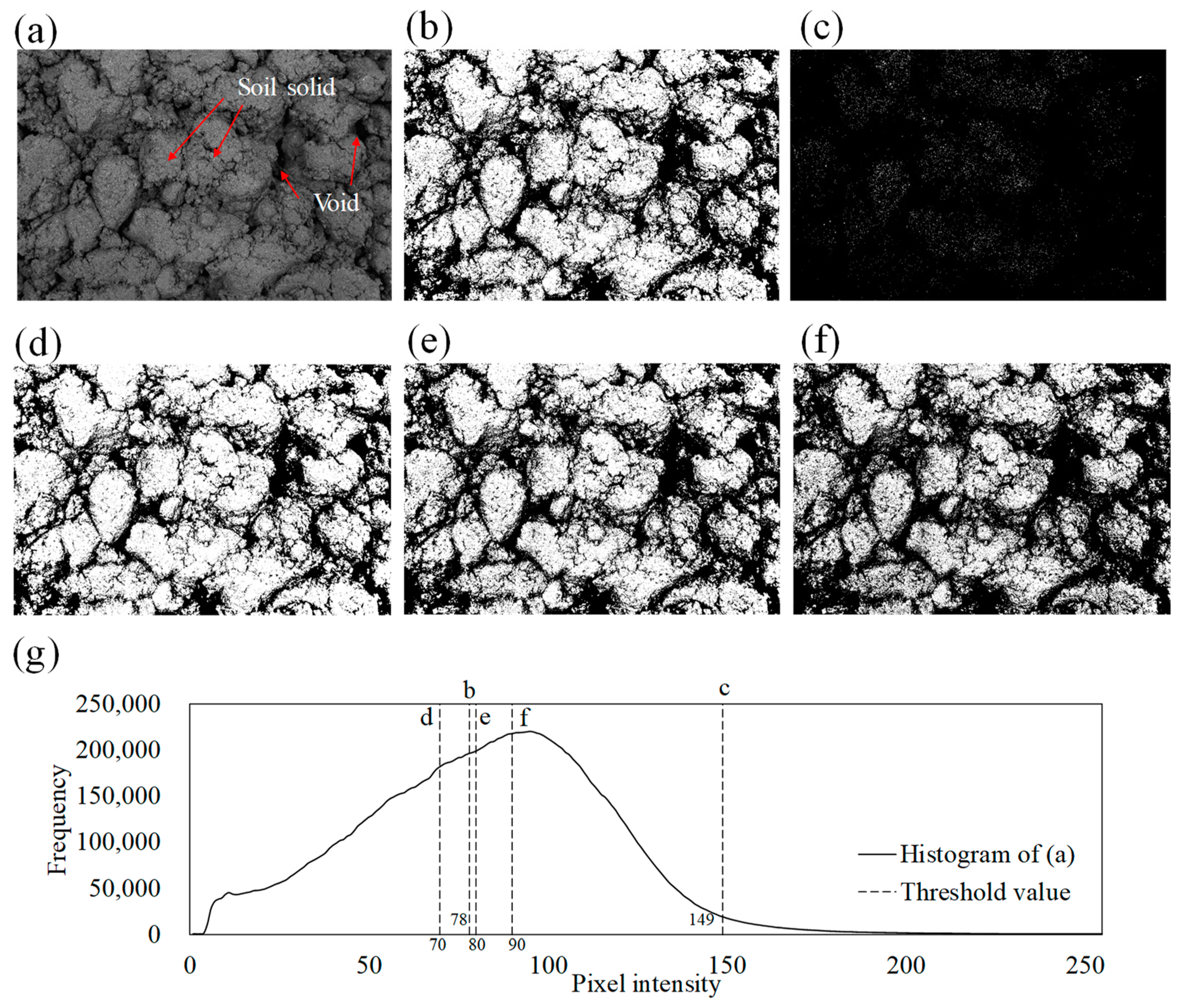
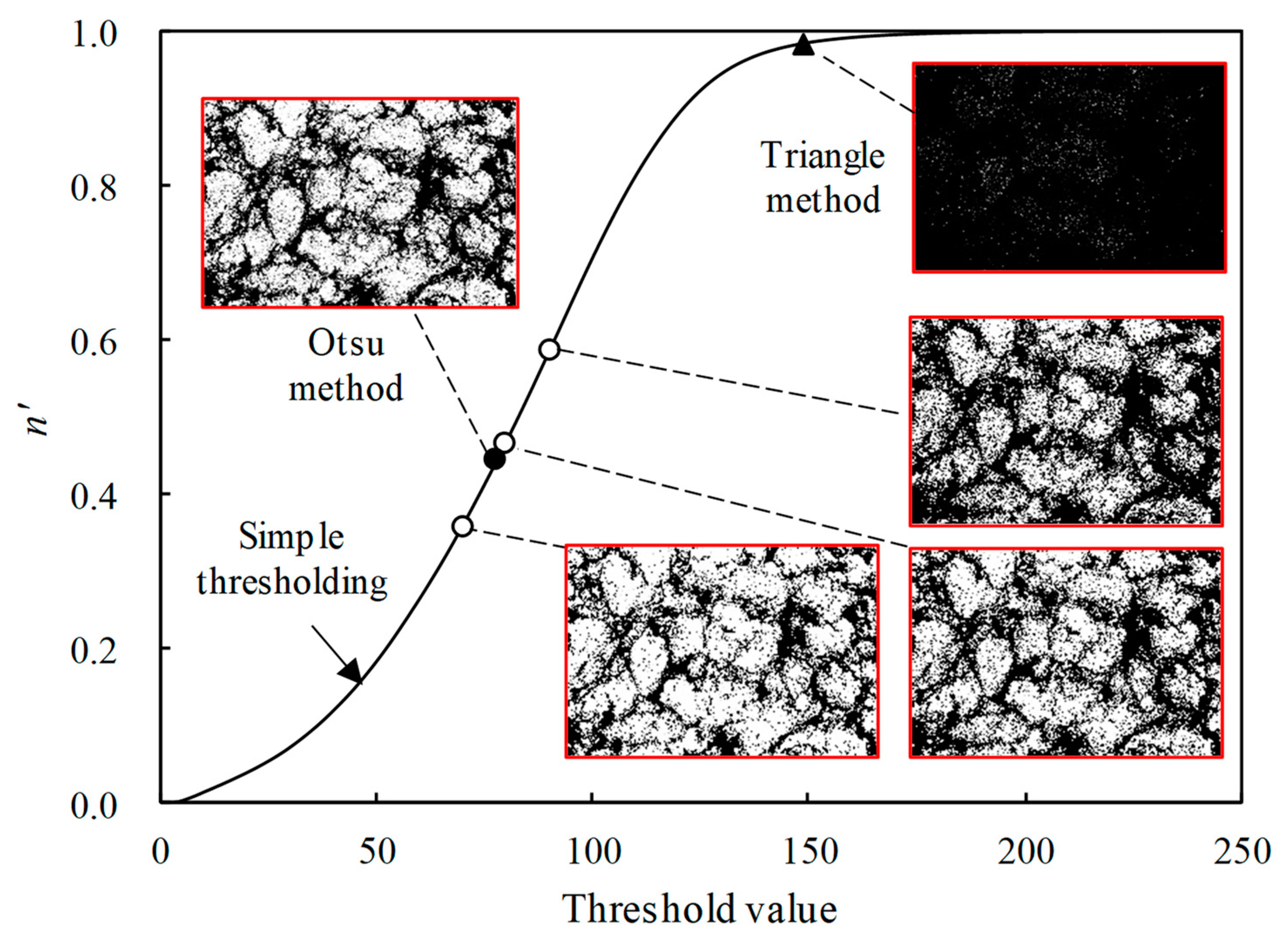
2.3. Image Thresholding

Image thresholding is one of the image segmentation methods. The image thresholding method divides an image into two regions based on a threshold value. The threshold value is an image intensity value between 0 and 255. After thresholding, if the intensity value of the image is greater than the threshold value, it is replaced with 255 (max value). If it is less than the threshold value, it is replaced with 0 (min value) [40]. Therefore, a threshold image is a binary image that has only two values of 255 (white) and 0 (black) for each pixel intensity [41]. It is important to determine the appropriate threshold value to achieve the desired result because the threshold value determines the outcome of the image thresholding. Image thresholding can be classified as simple thresholding or automatic thresholding. In simple thresholding, the threshold value is determined manually. Alternatively, automatic thresholding is a method of determining the threshold value according to preset algorithms.

In this study, image thresholding was used to distinguish between the soil solid and the void. Three thresholding methods were used to threshold the soil images: simple thresholding, the Otsu method, and the Triangle method. The Otsu method and the Triangle method are representative automatic thresholding methods. The Otsu method is a famous automatic thresholding method that returns a single threshold value determined by minimizing the intraclass intensity variance, or equivalently, by maximizing the interclass variance [42]. The Triangle method is an algorithm for finding the end of an image histogram and it determines the threshold value by normalizing the height and dynamic range of the histogram [43].

2.4. Image Processing

The binary image obtained as a result of image thresholding is used to compute $n^{\prime }$. The calculation process of $n^{\prime }$ is as follows. For image processing, we used the OpenCV (Open Computer Vision) library in Python (www.python.org). The OpenCV library includes many functions for image processing, and it also includes the three thresholding methods used in this study [44,45]. The original digital image is an RGB image comprising three channels of red, green, and blue. The original digital image was converted into an 8-bit grayscale image. The converted grayscale image was used for thresholding. Image thresholding is performed based on the determined threshold value. In simple thresholding, the threshold value is determined with an arbitrary value, and in the Otsu and Triangle method, it is determined according to each algorithm. Pixels with an image intensity of 255 are a soil solid, and pixels with an image intensity of 0 are a void. Then, $N_{void}$ is determined by counting the pixels with image intensity = 0. Additionally, $N_{void}$ can be computed as the sum of the frequencies in the histogram of a grayscale image that are less than a threshold value. The digital image used in this study has a total of 17,915,904 pixels, 5184 horizontal and 3456 vertical. Therefore, $N_{total}$ is fixed at 17,915,904. Finally, $n^{\prime }$ can be calculated according to Equation (7).

3. Results

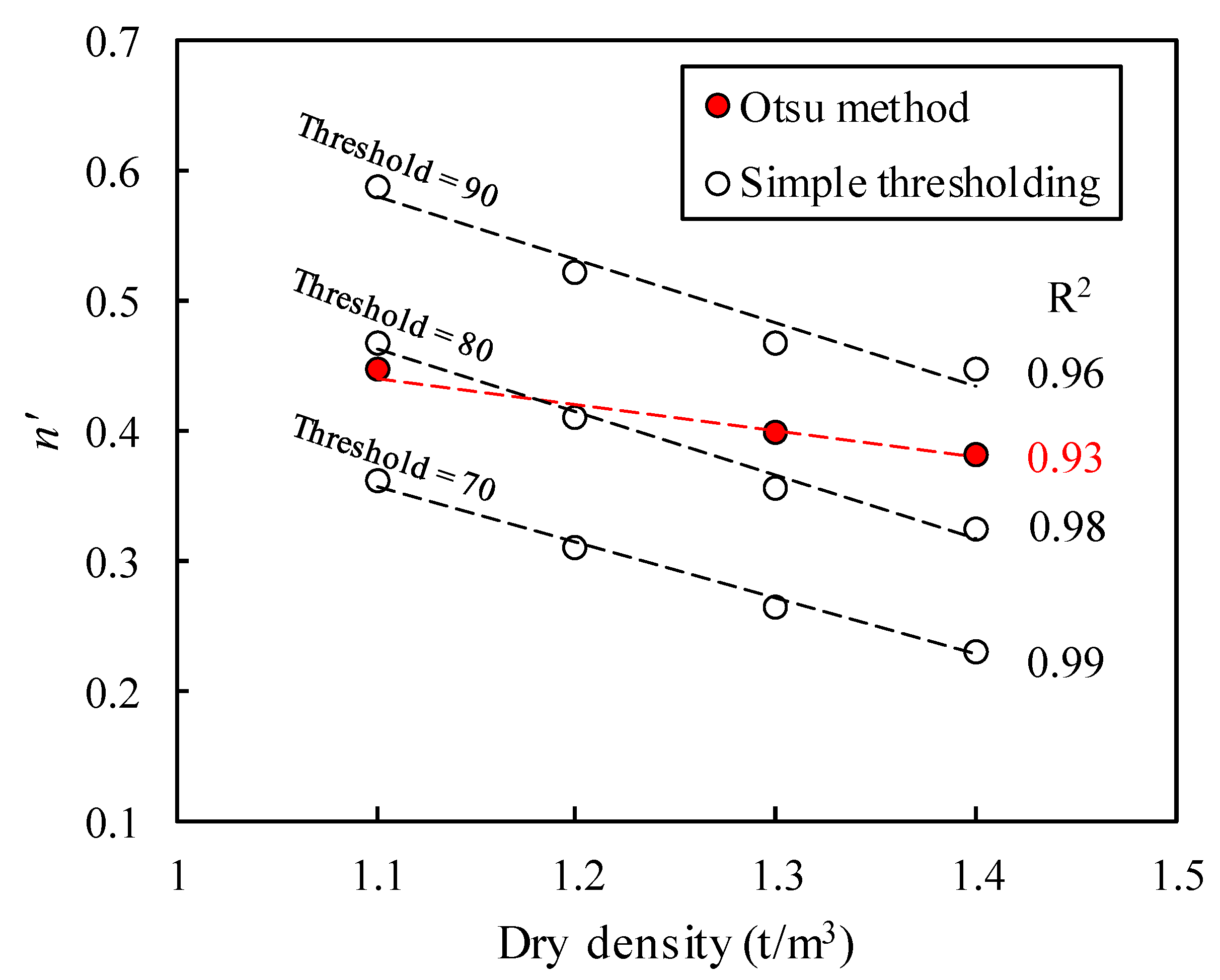
3.1. Dry Density Prediction by Thresholding of Soil Images

Figure 3 shows how the soil surface image and histogram change as the ${\rho }_d$ increases.

The soil texture is SiL and the water content is 25%. Soil solids are visible in Figure 3a, and voids, which are dark spaces between soil solids, are also present. Under the condition of low ${\rho }_d$, numerous voids are distributed, and as the ${\rho }_d$ increases, the distribution of the voids decreases. Figure 3b shows the histogram after converting the color image of Figure 3a to grayscale. The histogram is bell shaped, skewed to the right with one peak. For the intensity of the digital images and its histogram, 0 means black and 255 means white. As the ${\rho }_d$ increases, the frequency of the low intensity decreases and the frequency of the high intensity increases in the histogram. The average intensities of the histogram were 81.4, 85.5, 89.7, and 91.3, respectively. Comparing Figure 3a,b, the voids were distributed at a low intensity and the soil solid was distributed at a high intensity.

Figure 4 shows the result of thresholding a soil image.

Figure 4a is an image with a ${\rho }_d$ of 1.1 t/m³ in Figure 3a converted to grayscale. Figure 4b–f are threshold binary images, which are easier to distinguish between soil solids and voids than in the original grayscale image. Figure 4b,c show thresholding results using the Otsu method and Triangle method, respectively. Because both methods are automatic thresholding, the threshold value was automatically determined by the algorithm. In the case of the Otsu method, the soil solid and voids were well distinguished; however, it was difficult to distinguish them from the results of the Triangle method because the threshold value selected by the Triangle method was 149, which is far from the median value of the histogram. As a result, most of the pixels were classified as a void. Figure 4d–f show the results of simple thresholding with threshold values of 70, 80, and 90, respectively. Increasing the threshold value from 70 to 90 appears to noticeably increase the area of the voids displayed in black pixels on the image. Specifically, as the threshold value increases, $N_{void}$ and $n^{\prime }$ increase. Therefore, the accuracy of the density prediction will vary according to the threshold value.

Figure 5 shows the calculation results of $n^{\prime }$ according to the threshold value.

As the threshold value increased, $n^{\prime }$ increased from 0 to 1. This is the same as the possible range of $n$ values as shown in Figure 1. $n^{\prime }$ is almost close to 1 for threshold values of 170 and above. This is because the pixel intensity of a grayscale image is mostly below 170, as shown in Figure 4g. If the threshold value is the same, the result of the thresholding is the same. The threshold values determined by the Otsu method and the Triangle method were 78 and 149, respectively. So, the $n^{\prime }$ calculated from the binary images obtained by the Otsu method and the Triangle method showed the same value as the result of performing simple thresholding at the threshold values 78 and 149. Therefore, the thresholding results in Figure 4 all exist on the curve in Figure 5. Because the value of $n^{\prime }$ is determined by the threshold value, it is necessary to verify whether $n^{\prime }$ has a correlation with ${\rho }_d$ under various threshold values. According to the thresholding method, the result of the $n^{\prime }$ extracted from the same soil image was different, indicating that it is essential to determine an appropriate thresholding method for evaluating soil voids.

Figure 6 shows the relationship of ${\rho }_d$ and $n^{\prime }$ calculated with the images of Figure 1.

In the Otsu method, as the ${\rho }_d$ increases from 1.1 t/m³ to 1.2, 1.3, and 1.4 t/m³, the threshold values of 78, 80, 84, and 85 were selected, respectively. The coefficient of determination ($R^2$) of simple thresholding was greater than that of the Otsu method. As a result of this example image set, using a single threshold value gave better results than automatically determined by the Otsu method. However, results may vary in other soil conditions.

The correlation coefficients of ${\rho }_d$ and $n^{\prime }$ under various soil conditions are summarized in

Table 2. Correlation coefficient of the dry density and $n^{\prime }$ under various soil conditions.

Soil Condition		$\mathbf{Correlation}\mathbf{Coefficients}\mathbf{of}{\mathit{\rho }}_{\mathit{d}}$$\mathbf{and}{\mathit{n}}^{\mathbf{\prime }}$
Texture	Water Content (%)	Simple Thresholding			Otsu Method	Triangle Method
		70	80	90
SL	5	−0.69	−0.73	−0.77	0.94	−0.45
	10	−0.98	−0.98	−0.98	0.63	−0.95
	15	−0.97	−0.97	−0.97	−0.86	−0.86
	20	−0.99	−0.99	−0.99	−0.99	−0.83
	25	−0.97	−0.96	−0.95	−0.86	−0.85
L	5	−0.82	−0.84	−0.87	0.33	−0.77
	10	−0.91	−0.93	−0.94	0.76	−0.82
	15	−0.97	−0.98	−0.98	−0.89	−0.95
	20	−0.98	−0.98	−0.97	−0.96	−0.15
	25	−0.99	−0.99	−0.99	−0.97	−0.83
SiL	5	−0.91	−0.93	−0.94	0.24	−0.87
	10	−0.97	−0.98	−0.98	−0.69	−0.86
	15	−0.97	−0.96	−0.95	0.30	−0.95
	20	−0.97	−0.97	−0.96	−0.93	−0.94
	25	−0.90	−0.88	−0.84	−0.90	−0.80
SiCL	5	−0.55	−0.56	−0.59	0.21	−0.22
	10	−0.78	−0.79	−0.80	0.92	−0.81
	15	−0.61	−0.64	−0.67	0.80	−0.72
	20	−0.98	−0.98	−0.97	−0.97	−0.71
	25	−0.98	−0.98	−0.98	−0.98	−0.95
Average		-0.89	−0.90	−0.90	−0.24	−0.77

.

Twelve digital images were used to calculate one correlation coefficient. Each set of 12 images was produced by triplicate soil samples with dry densities of 1.1, 1.2, 1.3, and 1.4 t/m³ under one water content condition. For the Otsu method and Triangle method, $n^{\prime }$ was calculated according to the threshold value automatically selected according to the algorithm. According to Equation (5), $n$ and ${\rho }_d$ have a proportional relationship with −1 as the proportionality constant. Therefore, the closer the correlation coefficient is to −1, the better the ${\rho }_d$ prediction using $n^{\prime }$. Table 2 shows that ${\rho }_d$ and $n^{\prime }$ show a strong negative correlation in all thresholding methods at a water content of 20% or greater, indicating that ${\rho }_d$ can be predicted using $n^{\prime }$. However, when the water content is less than 15%, there is no correlation or a positive correlation, which means that these threshold methods cannot be used robustly for soil density prediction. Additionally, the determination of most proper threshold values for simple thresholding is still a problem. Therefore, it is necessary to derive new predictors of ${\rho }_d$.

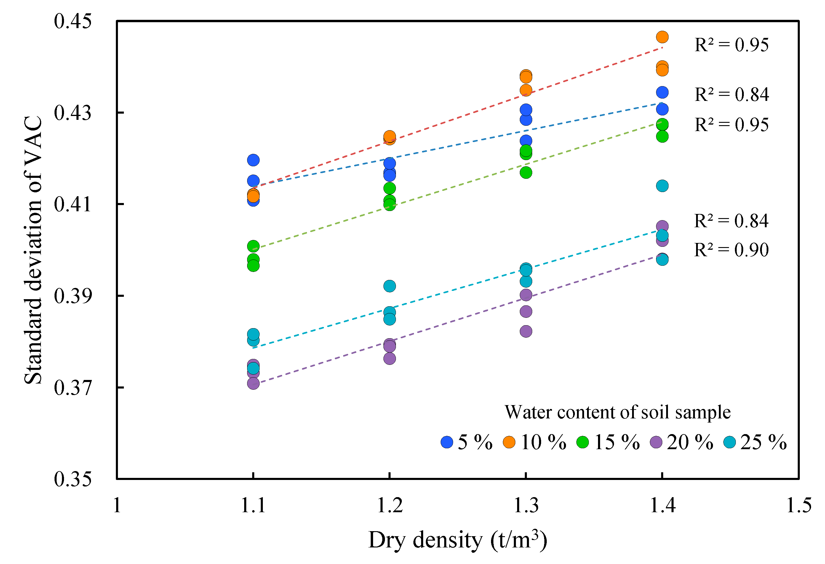
3.2. New Approach for the Dry Density Prediction Using Soil Image Properties

The $n^{\prime }$ calculated with every threshold value through simple thresholding is shown in Figure 7.

Depending on the threshold value, $n\prime$ shows an increasing curve in the form of a cumulative distribution function (CDF). As the ${\rho }_d$ increases, the graph moves downward. At the same threshold value, the higher the ${\rho }_d$, the lower $n^{\prime }$. Because $n^{\prime }$ represents the void area in the soil image, the graph of the relationship between the threshold value and $n^{\prime }$ was named as the void area curve (VAC). A parameter representing the shape of the VAC was extracted based on the shape determinant factor of CDF. Standard deviation ($\sigma$) is the most representative parameter that determines the shape of the CDF. The standard deviation of VAC can be calculated by Equation (8).

$${\sigma }_{n^{\prime }}=\sqrt{\frac{\sum _{i=1}^N({n^{\prime }}_i-\overline{n^{\prime }}{)}^2}{N}}$$

(8)

where ${\sigma }_{n^{\prime }}$ is the standard deviation of VAC, ${n^{\prime }}_i$ is $n^{\prime }$ at the threshold value = i, $\overline{n^{\prime }}$ is the mean value of $n^{\prime }$, and $N$ is the sample size. The relationship between the standard deviation of VAC and the ${\rho }_d$ for soil SiL under various water content conditions is shown in Figure 8.

${\sigma }_{n^{\prime }}$ has a strong correlation with ${\rho }_d$. Compared with the results of simple thresholding, it is at a similar level of correlation; however, it is highly practical in that it does not require the determination of the threshold value. As a result of the analysis, the standard deviation represents the shape of the VAC well. However, it is necessary to verify that the correlation between the standard deviation of VAC and ${\rho }_d$ is consistently maintained under various soil conditions.

Table 3. RMSE of the dry density prediction by soil images under various soil conditions.

Soil Condition		RMSE (t/m3)
Texture	Water Content (%)	${\mathit{\sigma }}_{{\mathit{n}}^{\mathbf{\prime }}}$	Simple Thresholding			Otsu Method	Triangle Method
			70	80	90
SL	5	0.067	0.081	0.077	0.072	0.039	0.100
	10	0.016	0.023	0.022	0.024	0.087	0.034
	15	0.024	0.026	0.027	0.029	0.057	0.056
	20	0.011	0.015	0.016	0.017	0.012	0.063
	25	0.024	0.028	0.031	0.034	0.057	0.059
L	5	0.110	0.064	0.060	0.056	0.106	0.071
	10	0.041	0.045	0.042	0.039	0.072	0.064
	15	0.016	0.027	0.024	0.023	0.052	0.034
	20	0.024	0.022	0.023	0.025	0.030	0.111
	25	0.014	0.015	0.015	0.015	0.027	0.062
SiL	5	0.045	0.045	0.042	0.040	0.108	0.054
	10	0.026	0.025	0.023	0.022	0.081	0.057
	15	0.025	0.029	0.030	0.035	0.107	0.035
	20	0.036	0.027	0.027	0.030	0.041	0.038
	25	0.044	0.049	0.054	0.061	0.050	0.068
SiCL	5	0.077	0.094	0.093	0.090	0.109	0.109
	10	0.042	0.070	0.068	0.067	0.044	0.066
	15	0.061	0.089	0.086	0.083	0.067	0.078
	20	0.018	0.023	0.024	0.026	0.026	0.078
	25	0.020	0.021	0.021	0.021	0.023	0.034
Average		0.037	0.041	0.040	0.040	0.060	0.064

shows the root mean square error (RMSE) of the ${\rho }_d$ prediction using the soil images.

4. Discussion

4.1. Accuracy of the Density Prediction Using Void Area Curve

In this study, we aimed to improve the existing density prediction method that depends on the value of the threshold value. Therefore, instead of selecting a single threshold value, $n^{\prime }$ was calculated for all possible threshold values, which is called the void area curve. The shape of the histogram in Figure 4g is unimodal because the object (soil solid) and background (void) are not clearly distinguishable in the digital image of the soil. This study does not seek a thresholding method that can perfectly distinguish between a void and a soil solid, but rather predicts density using features from the relationship between $n^{\prime }$ and the threshold value. This is because the main goal is not to obtain an image with flawless void and soil solid separation, but to obtain a good estimation of the dry density. The void area curve method proposed in this study seems to serve this purpose well. The analysis showed that the standard deviation of the void area curve can be used to predict the ${\rho }_d$ with high accuracy. As shown in Table 3, the accuracy of ${\rho }_d$ prediction varies depending on the threshold value. A major advantage of the method proposed in this study is that it can perform robust analysis, unlike existing methods whose accuracy may vary depending on the threshold value.

The accuracy of the ${\rho }_d$ test and prediction results are summarized in

Table 4. Accuracy of the dry density test and prediction.

Method		RMSE (t/m3)	Range of Water Content (%)	Number of Tests	Texture
Field density test [6]	Sand Cone	0.025	8.3 to 13.3	49	Sandy loam
	Nuclear	0.042		253
	Drive Cylinder	0.057		60
Kim et al. [28]	Image analysis using convolutional neural network	0.044 to 0.107	5 to 25	80	Sandy loam, Loam, Silt loam and Silty clay loam
Kim et al. [29]	Image analysis using deep neural network	0.080	1.2 to 22.3	74	Loamy sand, Sandy loam, Silt loam
This study	Image analysis using void area curve	0.037	5 to 25	240	Sandy loam, Loam, Silt loam and Silty clay loam

. Noorany et al. [6] conducted a precise test using a large soil tank with a diameter of 122 cm and a height of 100 cm in laboratory conditions to verify the accuracy of the field density test. In addition, Kim et al. [28,29] performed digital image-based density prediction of soil via a convolutional neural network and deep neural network.

The RMSE of ${\rho }_d$ prediction using ${\sigma }_{n^{\prime }}$ was 0.037 t/m³, which was superior to other experimental methods except sand cone. Additionally, the range of water content during the ${\rho }_d$ tests was 8.3–13.3%; however, in this study, soils with a water content from 5% to 25% were used. In particular, four textures of soil according to the USDA classification method were used. Therefore, the method has a high level of accuracy similar to that of the existing test method even when considering several water contents and soil textures.

As summarized in Table 4, it also showed better accuracy than studies that used deep learning to analyze images. The convolutional neural network had an RMSE of 0.044 to 0.107 t/m³, while the deep neural network had an RMSE of 0.080 t/m³. This shows that ${\sigma }_{n^{\prime }}$ is a better indicator for predicting ${\rho }_d$ than the image features used in the deep learning model. Therefore, the ${\rho }_d$ prediction method using ${\sigma }_{n^{\prime }}$ can be widely used as a method for predicting ${\rho }_d$ because it shows a similar level of accuracy to the existing test method and a higher accuracy than other analysis methods. In this study, only one variable (${\sigma }_{n^{\prime }}$) was used to predict ${\rho }_d$. Since various other features can be extracted from soil surface images, it is expected that a multivariate analysis with additional features will improve the accuracy.

Comparing the accuracy of the soil density analysis based on vis-NIR spectroscopy [32,33,34] with the results of this study, the RMSE is lower and the R² is higher, indicating good accuracy. Davari et al. [31] reported that vis-NIR spectroscopy and PLSR successfully predicted various soil properties, but the prediction accuracy was poor for bulk density with a validation R² of 0.35. The main advantage of the results of this study compared to the analysis based on vis-NIR spectroscopy is that a high level of density prediction is possible with a common digital camera. Given the widespread availability of digital cameras, this could have very broad applications. However, the digital images used in this study were acquired in a laboratory and their applicability in the field is still unknown. Therefore, further research in the field is needed to further enhance the versatility of this study.

4.2. Practical Considerations and Limitations

In this study, we proposed the VAC from a soil surface image that can be used to predict the ${\rho }_d$ in agricultural lands. The limitations of this study are summarized as follows.

Four soil textures, SL, L, SiL, and SiCL, were analyzed, ranging from SL with a high sand content to SiCL with a high clay and silt content, but the prediction performance may vary in soils with different textures. In particular, it is considered that the accuracy may decrease in soil textures such as sandy clay, silty clay, and clay where the clay content is higher than SiCL. This is because macropores may not be well represented at higher clay contents.

It is also likely that the accuracy of the prediction will decrease if the digital image quality is poor. The histogram of the sample image presented in Figure 3b shows that the intensity of the pixels is well distributed. If the pixels were over- or under-lighted due to a camera or lighting setup mistake, the histogram would show peaks skewed towards 0 or 255. In this case, the shape of the VAC may be distorted, which will reduce its accuracy.

The study was conducted on soil surface images; therefore, the data acquisition for subsurface soils was limited. Similar to the conventional in situ density test method, image analysis can be attempted after removing the upper soil; however, verification is required. In agricultural soil management, soil properties in the root zone directly affect crop growth [46]. Therefore, it is necessary to verify the applicability of the image analysis method to the subsoil region.

Regarding the compaction of the sample, the entire surface layer was compacted in this study to make the surface layer even. In the soil surface layer, compaction may occur by the operation of agricultural machinery [47,48]. In addition, it may be difficult to obtain an image when the surface layer is obstructed by vegetation or other obstacles. Therefore, for field applications, it is necessary to exclude unnecessary regions from the surface layer image.

Cameras can show different colors of the same object according to settings such as color temperature and exposure. In this study, digital images were acquired under fixed lighting conditions in an indoor studio. Because the lighting conditions of the agricultural lands continuously change depending on the time of day and weather conditions, it would be desirable to install a darkroom to control the lighting conditions outside the camera. It is necessary to develop a method that can be used universally under various lighting conditions.

In addition, it is necessary to review the optimal resolution of the soil surface image. Unlike other objects, soil is a material whose size affects its properties. Even with the same camera, the size of an object varies depending on the working distance. When shooting from a close distance, the soil solid and void space can be observed in more detail. Conversely, when shooting from a distance, even though a relatively larger area of soil surface can be observed, the resolution is reduced. As a result, a review of the optimal resolution for soil density prediction is needed.

5. Conclusions

In this study, we introduced the void area curve (VAC) as an innovative approach for accurately predicting soil density based on digital image analysis. The VAC methodology represents a significant departure from conventional techniques, offering a novel perspective on soil density prediction. While our investigation highlighted the Otsu method as the optimal choice among automatic thresholding methods, it was the simplicity and robustness of the $n^{\prime }$ metric calculated through simple thresholding that demonstrated a superior correlation with soil density. Recognizing the inherent complexities associated with threshold value selection, our research addressed this challenge by introducing the VAC. This method not only enhances the precision of soil density predictions but also eliminates the need for manual threshold determination.

A remarkable outcome of our study was the remarkable accuracy achieved in predicting the dry density of soil, through the standard deviation of the VAC. However, it is essential to acknowledge some limitations. The applicability of the VAC method may vary depending on soil types, and further research is needed to explore its performance under diverse geological conditions. Additionally, while the VAC simplifies threshold selection, fine-tuning for specific applications might still be necessary in some cases. In conclusion, the standard deviation of the VAC emerges as a powerful tool with the potential to revolutionize soil density prediction, offering a universally applicable approach. Future analyses should aim to refine the VAC’s applicability across soil types and investigate additional factors that may influence its predictive capabilities.

References

1. Logsdon, S.D.; Karlen, D.L. Bulk density as a soil quality indicator during conversion to no-tillage. Soil Tillage Res. 2004, 78, 143–149. [Google Scholar] [CrossRef]
2. Tang, A.M.; Cui, Y.-J.; Richard, G.; Défossez, P. A study on the air permeability as affected by compression of three French soils. Geoderma 2011, 162, 171–181. [Google Scholar] [CrossRef]
3. Tracy, S.R.; Black, C.R.; Roberts, J.A.; Mooney, S.J. Soil compaction: A review of past and present techniques for investigating effects on root growth. J. Sci. Food Agric. 2011, 91, 1528–1537. [Google Scholar] [CrossRef] [PubMed]
4. Czyż, E.A. Effects of traffic on soil aeration, bulk density and growth of spring barley. Soil Tillage Res. 2004, 79, 153–166. [Google Scholar] [CrossRef]
5. Watson, G.W.; Kelsey, P. The impact of soil compaction on soil aeration and fine root density of Quercus palustris. Urban For. Urban Green. 2006, 4, 69–74. [Google Scholar] [CrossRef]
6. Noorany, I.; Gardner, W.S.; Corley, D.J.; Brown, J.L. Variability in field density tests. ASTM Spec. Tech. Publ. 2000, 1384, 58–71. [Google Scholar]
7. Lampurlanés, J.; Cantero-Martínez, C. Soil bulk density and penetration resistance under different tillage and crop management systems and their relationship with barley root growth. Agron. J. 2003, 95, 526–536. [Google Scholar] [CrossRef]
8. Liu, J.; Shi, B.; Sun, M.-Y.; Zhang, C.-C.; Guo, J.-Y. In-situ soil dry density estimation using actively heated fiber-optic FBG method. Measurement 2021, 185, 110037. [Google Scholar] [CrossRef]
9. Brewer, R. Fabric and mineral analysis of soils. Soil Sci. 1965, 100, 73. [Google Scholar] [CrossRef]
10. Van den Akker, J.; Soane, B. Compaction. In Encyclopedia of Soils in the Environment; Hillel, D., Ed.; Elsevier: Oxford, UK, 2005; pp. 285–293. [Google Scholar]
11. Ruser, R.; Sehy, U.; Weber, A.; Gutser, R.; Munch, J. Main driving variables and effect of soil management on climate or ecosystem-relevant trace gas fluxes from fields of the FAM. In Perspectives for Agroecosystem Management; Elsevier: Amsterdam, The Netherlands, 2008; pp. 79–120. [Google Scholar]
12. Ravikumar, R.; Arulmozhi, D.V. Digital image processing—A quick review. Int. J. Intell. Comput. Technol. (IJICT) 2019, 2, 11–19. [Google Scholar]
13. Adderley, W.P.; Simpson, I.A.; Davidson, D.A. Colour description and quantification in mosaic images of soil thin sections. Geoderma 2002, 108, 181–195. [Google Scholar] [CrossRef]
14. Bruneau, P.M.; Davidson, D.A.; Grieve, I.C. An evaluation of image analysis for measuring changes in void space and excremental features on soil thin sections in an upland grassland soil. Geoderma 2004, 120, 165–175. [Google Scholar] [CrossRef]
15. Peng, X.; Horn, R.; Peth, S.; Smucker, A. Quantification of soil shrinkage in 2D by digital image processing of soil surface. Soil Tillage Res. 2006, 91, 173–180. [Google Scholar] [CrossRef]
16. Prats-Montalbán, J.M.; de Juan, A.; Ferrer, A. Multivariate image analysis: A review with applications. Chemom. Intell. Lab. Syst. 2011, 107, 1–23. [Google Scholar] [CrossRef]
17. Chitradevi, B.; Srimathi, P. An overview on image processing techniques. Int. J. Innov. Res. Comput. Commun. Eng. 2014, 2, 6466–6472. [Google Scholar]
18. Ren, J.; Li, X.; Zhao, K. Quantitative analysis of relationships between crack characteristics and properties of soda-saline soils in Songnen Plain, China. Chin. Geogr. Sci. 2015, 25, 591–601. [Google Scholar] [CrossRef]
19. Aydemir, S.; Keskin, S.; Drees, L. Quantification of soil features using digital image processing (DIP) techniques. Geoderma 2004, 119, 1–8. [Google Scholar] [CrossRef]
20. O’Donnell, T.K.; Goyne, K.W.; Miles, R.J.; Baffaut, C.; Anderson, S.H.; Sudduth, K.A. Identification and quantification of soil redoximorphic features by digital image processing. Geoderma 2010, 157, 86–96. [Google Scholar] [CrossRef]
21. Ohm, H.-S.; Hryciw, R.D. Size distribution of coarse-grained soil by sedimaging. J. Geotech. Geoenviron. Eng. 2014, 140, 04013053. [Google Scholar] [CrossRef]
22. Idowu, K.A.; Olaleye, B.M.; Saliu, M.A. Analysis of blasted rocks fragmentation using digital image processing (Case study: Limestone quarry of Obajana Cement Company). Min. Miner. Depos. 2021, 15, 34–42. [Google Scholar] [CrossRef]
23. Elliot, T.R.; Heck, R.J. A comparison of optical and X-ray CT technique for void analysis in soil thin section. Geoderma 2007, 141, 60–70. [Google Scholar] [CrossRef]
24. Abd El-Halim, A. Image processing technique to assess the use of sugarcane pith to mitigate clayey soil cracks: Laboratory experiment. Soil Tillage Res. 2017, 169, 138–145. [Google Scholar] [CrossRef]
25. Li, H.-D.; Tang, C.-S.; Cheng, Q.; Li, S.-J.; Gong, X.-P.; Shi, B. Tensile strength of clayey soil and the strain analysis based on image processing techniques. Eng. Geol. 2019, 253, 137–148. [Google Scholar] [CrossRef]
26. Pham, D.L.; Xu, C.; Prince, J.L. A survey of current methods in medical image segmentation. Annu. Rev. Biomed. Eng. 2000, 2, 315–337. [Google Scholar] [CrossRef] [PubMed]
27. Landis, E.N.; Keane, D.T. X-ray microtomography. Mater. Charact. 2010, 61, 1305–1316. [Google Scholar] [CrossRef]
28. Kim, D.; Kim, T.; Jeon, J.; Son, Y. Convolutional Neural Network-Based Soil Water Content and Density Prediction Model for Agricultural Land Using Soil Surface Images. Appl. Sci. 2023, 13, 2936. [Google Scholar] [CrossRef]
29. Kim, D.; Kim, T.; Jeon, J.; Son, Y. Soil-Surface-Image-Feature-Based Rapid Prediction of Soil Water Content and Bulk Density Using a Deep Neural Network. Appl. Sci. 2023, 13, 4430. [Google Scholar] [CrossRef]
30. Yang, J.; Wang, X.; Wang, R.; Wang, H. Combination of convolutional neural networks and recurrent neural networks for predicting soil properties using Vis–NIR spectroscopy. Geoderma 2020, 380, 114616. [Google Scholar] [CrossRef]
31. Davari, M.; Karimi, S.A.; Bahrami, H.A.; Hossaini, S.M.T.; Fahmideh, S. Simultaneous prediction of several soil properties related to engineering uses based on laboratory Vis-NIR reflectance spectroscopy. Catena 2021, 197, 104987. [Google Scholar] [CrossRef]
32. Lobsey, C.; Viscarra Rossel, R. Sensing of soil bulk density for more accurate carbon accounting. Eur. J. Soil Sci. 2016, 67, 504–513. [Google Scholar] [CrossRef]
33. Xu, D.; Ma, W.; Chen, S.; Jiang, Q.; He, K.; Shi, Z. Assessment of important soil properties related to Chinese Soil Taxonomy based on vis–NIR reflectance spectroscopy. Comput. Electron. Agric. 2018, 144, 1–8. [Google Scholar] [CrossRef]
34. Katuwal, S.; Knadel, M.; Norgaard, T.; Moldrup, P.; Greve, M.H.; de Jonge, L.W. Predicting the dry bulk density of soils across Denmark: Comparison of single-parameter, multi-parameter, and vis–NIR based models. Geoderma 2020, 361, 114080. [Google Scholar] [CrossRef]
35. Askari, M.S.; Cui, J.; O’Rourke, S.M.; Holden, N.M. Evaluation of soil structural quality using VIS–NIR spectra. Soil Tillage Res. 2015, 146, 108–117. [Google Scholar] [CrossRef]
36. Sezgin, M.; Sankur, B. Survey over image thresholding techniques and quantitative performance evaluation. J. Electron. Imaging 2004, 13, 146–165. [Google Scholar]
37. Passoni, S.; Borges, F.d.S.; Pires, L.F.; Saab, S.d.C.; Cooper, M. Software Image J to study soil pore distribution. Ciência E Agrotecnologia 2014, 38, 122–128. [Google Scholar] [CrossRef]
38. Smet, S.; Plougonven, E.; Leonard, A.; Degré, A.; Beckers, E. X-ray µCT: How soil pore space description can be altered by image processing. Vadose Zone J. 2018, 17, 1–14. [Google Scholar] [CrossRef]
39. Lambe, T.W.; Whitman, R.V. Soil Mechanics; John Wiley & Sons: Hoboken, NJ, USA, 1991; Volume 10. [Google Scholar]
40. de Faria Borges, L.P.; de Moraes, R.M.; Crestana, S.; Cavalcante, A.L.B. Geometric features and fractal nature of soil analyzed by X-ray microtomography image processing. Int. J. Geomech. 2019, 19, 04019088. [Google Scholar] [CrossRef]
41. Jaber, A.G.; Eesa, A.M.; Jasim, B.S. Image segmentation by using thresholding technique in two stages. Period. Eng. Nat. Sci. 2021, 9, 531–541. [Google Scholar] [CrossRef]
42. Otsu, N. A threshold selection method from gray-level histograms. IEEE Trans. Syst. Man Cybern. 1979, 9, 62–66. [Google Scholar] [CrossRef]
43. Zack, G.W.; Rogers, W.E.; Latt, S.A. Automatic measurement of sister chromatid exchange frequency. J. Histochem. Cytochem. 1977, 25, 741–753. [Google Scholar] [CrossRef]
44. Xie, G.; Lu, W. Image edge detection based on opencv. Int. J. Electron. Electr. Eng. 2013, 1, 104–106. [Google Scholar] [CrossRef]
45. Yaru, Y.; Jialin, Z. Algorithm of fingerprint extraction and implementation based on OpenCV. In Proceedings of the 2017 2nd International Conference on Image, Vision and Computing (ICIVC), Chengdu, China, 2–4 June 2017; pp. 163–167. [Google Scholar]
46. Zhao, P.-F.; Wang, Y.-Q.; Yan, S.-X.; Fan, L.-F.; Wang, Z.-Y.; Zhou, Q.; Yao, J.-P.; Cheng, Q.; Wang, Z.-Y.; Huang, L. Electrical imaging of plant root zone: A review. Comput. Electron. Agric. 2019, 167, 105058. [Google Scholar] [CrossRef]
47. Ungureanu, N.; Croitoru, Ş.; Biriş, S.; Voicu, G.; Vlăduţ, V.; Selvi, K.; Boruz, S.; Marin, E.; Matache, M.; Manea, D. Agricultural soil compaction under the action of agricultural machinery. In Proceedings of the Symposium “Actual Tasks on Agricultural Engineering”, Opatija, Croatia, 24–25 February 2015. [Google Scholar]
48. Kenarsari, A.E.; Vitton, S.J.; Beard, J.E. Creating 3D models of tractor tire footprints using close-range digital photogrammetry. J. Terramechanics 2017, 74, 1–11. [Google Scholar] [CrossRef]
Figure 1. Changes in the void ratio and porosity according to the volume composition of the soil mass.
Applsci 13 10484 g001
Figure 2. Changes in the void ratio and porosity according to dry density.
Applsci 13 10484 g002
Figure 3. Soil images and histogram under various dry densities: (a) original color images and (b) histogram of grayscale images.
Applsci 13 10484 g003
Figure 4. The thresholding of the sample image: (a) grayscale image, (b) result of the Otsu method, (c) result of the Triangle method, and (df) results of simple thresholding. (g) Histogram of (a) and threshold values.
Applsci 13 10484 g004
Figure 5. n of the threshold soil images. The soil images are the same as in Figure 4b–f. n of the simple thresholding is calculated at one interval of the threshold values from 0 to 255.
Applsci 13 10484 g005
Figure 6. The relationship of ρ d and n according to thresholding methods.
Applsci 13 10484 g006
Figure 7. n of soil images with various dry densities.
Applsci 13 10484 g007
Figure 8. The relationship between the dry density and standard deviation of VAC.
Applsci 13 10484 g008