Hybrid LSTM Model to Predict the Level of Air Pollution in Montenegro

Abstract

Air pollution is a critical environmental concern that poses significant health risks and affects multiple aspects of human life. ML algorithms provide promising results for air pollution prediction. In the existing scientific literature, Long Short-Term Memory (LSTM) predictive models, as well as their combination with other statistical and machine learning approaches, have been utilized for air pollution prediction. However, these combined algorithms may not always provide suitable results due to the stochastic nature of the factors that influence air pollution, improper hyperparameter configurations, or inadequate datasets and data characterized by great variability and extreme dispersion. The focus of this paper is applying and comparing the performance of Support Vector Machine and hybrid LSTM regression models for air pollution prediction. To identify optimal hyperparameters for the LSTM model, a hybridization with the Genetic Algorithm is proposed. To mitigate the risk of overfitting, the bagging technique is employed on the best LSTM model. The proposed predicitive model aims to determine the Common Air Quality Index level for the next hour in Niksic, Montenegro. With the hybridization of the LSTM algorithm and by applying the bagging technique, our approach aims to significantly enhance the accuracy and reliability of hourly air pollution prediction. The major contribution of this paper is in the application of advanced machine learning analysis and the combination of the LSTM, Genetic Algorithm, and bagging techniques, which have not been previously employed in the analysis of air pollution in Montenegro. The proposed model will be made available to interested management structures, local governments, national entities, or other relevant institutions, empowering them to make effective pollution level predictions and take appropriate measures.

1. Introduction

Air pollution is a concerning global issue, with approximately 1.3 million annual deaths attributed to it, according to the World Health Organization (WHO) [1]. Air quality assessment plays a vital role in monitoring and managing pollution levels. WHO data reveal that air pollution exceeding the recommended limits affects nearly the entire global population (99%), with a significant impact in low- and middle-income countries. It is crucial to anticipate and prepare for fluctuations in pollution levels to effectively mitigate the adverse effects of air pollution. Improving air quality not only enhances public health but also contributes to mitigating climate change, as air quality is closely interconnected with our planet’s climate and the health of its ecosystems. By reducing air pollution, we can alleviate the burden of diseases associated with air pollution and make long-term contributions to climate change mitigation efforts.

Since 2005, the Common Air Quality Index (CAQI) has been employed in Europe as a comprehensive and standardized metric to evaluate and communicate air quality levels to the general public [2]. It provides a simplified and easily understandable representation of air pollution levels, making it easier for individuals to make informed decisions regarding their health and well-being. The CAQI is based on the measurement of several air pollutants that are known to have detrimental effects on human health, including particulate matter (PM_2.5 and PM₁₀), nitrogen dioxide (NO₂), ozone (O₃), carbon monoxide (CO), and sulfur dioxide (SO₂) [3]. These pollutants are commonly monitored by air quality monitoring stations located in various regions. The CAQI is designed to provide a numerical value or color-coded scale that corresponds to the air quality level.

Typically, the CAQI scale ranges from 0 to 100 and it is divided into several categories, such as very low, low, medium, high, and very high [4], and the visual color scale is presented from green to red. To calculate the CAQI value, individual pollutant concentrations are first converted into indexes using predefined equations that are based on value interpolation. These indexes are then combined, weighted, and transformed into a single CAQI value. The weighting factors assigned to each pollutant are determined based on their relative health impacts.

The CAQI is a valuable tool in terms of raising awareness about air pollution and its potential health risks. It enables policymakers, environmental agencies, and the general public to monitor and address air quality issues effectively. Additionally, the CAQI facilitates the comparison of air quality between different locations and allows for long-term trend analysis, aiding in the formulation of targeted strategies for air pollution control and mitigation.

The advancement of machine learning (ML) techniques, including deep learning, has opened up new opportunities to enhance air quality research [5]. Among these techniques, the Support Vector Machine (SVM) has demonstrated promising outcomes in diverse domains. As a supervised learning algorithm, SVM is designed in the manner that it can identify optimal hyperplanes to enable the formation of data classes. In the context of air pollution prediction, SVM can learn complex patterns and relationships from historical pollution data and meteorological variables [6]. On the other hand, LSTM represents a type of recurrent neural network known for its effectiveness in modeling sequential data [7]. It can capture long-term dependencies and temporal patterns, making it suitable for time series forecasting tasks such as air pollution prediction.

The hybridization of ML algorithms with other techniques yields good results, especially when it comes to metaheuristic algorithms. Hybridization allows the faster convergence of algorithms and increases the prediction accuracy of ML algorithms. There is a wide range of metaheuristic algorithms [8] and one of the most commonly used is the Genetic Algorithm (GA), which is inspired by the process of natural selection [9]. It can effectively search for optimal or suboptimal solutions in a large solution space.

Bagging is an ensemble learning technique that enhances predictions by consolidating multiple models trained on diverse subsets of data. By aggregating the predictions of individual models, bagging reduces overfitting and increases the stability and robustness of the algorithms. It helps to capture different patterns and relationships present in the data, increasing the model’s overall performance by enhancing accuracy, handling data noise, and increasing robustness [10].

This paper focuses on the development of an advanced hourly CAQI prediction model through the hybridization of metaheuristics, ML algorithms, and ensemble learning techniques. More precisely, three different techniques are combined: GA, the LSTM algorithm, and a bagging approach. To our knowledge, this combination of techniques has not been applied yet to air pollution analysis in Montenegro. Regarding the numerical results, a comparison with standard ML prediction algorithms (SVM) is made. Our results show that the proposed hybrid model significantly outperforms the SVM model in terms of accuracy and convergence.

2. Related Work

Recent studies have been focusing on sophisticated learning algorithms to enhance air quality evaluation and air pollution prediction. Drewil and Al-Bahadili [11] used the LSTM model in conjunction with GA to enhance the performance of air prediction models. The performance of the GA-LSTM model was evaluated and compared with models employing manual criteria. The results showed a significant improvement in LSTM performance with the integration of GA. Waseem et al. [12] chose to perform only PM_2.5 forecasting by applying deep learning techniques, among which the LSTM encoder–decoder variant showed promising results. In another study, Xayasouk et al. [13] examined the methods of predicting PM levels and showed that LSTM combined with deep autoencoder techniques showed slightly better performance than the typical LSTM model.

Triana and Osowski [14] employed bagging and boosting techniques for PM prediction. Their experiments demonstrated significant improvements in result quality when using bagging and boosting ensembles with weak predictors. The Mean Absolute Error was reduced by more than 30% for PM₁₀ and 20% for PM_2.5 compared to individual predictors. Liang et al. [15] developed multiple ML models, including adaptive boosting (AdaBoost), an artificial neural network (ANN), random forest (RF), a stacking ensemble, and SVM, for the prediction of air quality index levels over different time intervals (1 h, 8 h, and 24 h). The stacking ensemble, AdaBoost, and RF models showed the best prediction performance, although their forecasting accuracy varied across geographical regions. Madhuri et al. [16] used linear regression, SVM, decision tree, and RF models for air quality prediction. The RF model achieved the highest accuracy among the tested algorithms. Kumar and Pande [17] applied five different ML models to predict air quality. The authors showed that the strongest correlation between predicted and actual data was achieved by the XGBoost model. Sanjeev [18] conducted a study where a few standard classification models were applied to a dataset that included pollutant concentrations and meteorological data. Due to its robustness against overfitting, the RF classifier demonstrated superior performance compared to other classifiers.

In their review, Rybarczyk and Zalakeviciute [19] examined a collection of 46 highly relevant journal papers. The authors found that there were more studies focused on pollutants such as O₃, NO₂, PM₁₀, and PM_2.5, while fewer studies covered CAQI prediction. We refer interested readers to a comprehensive review [20] of 155 papers that provides a detailed analysis of air quality prediction using ML techniques.

3. Implementation Methodology

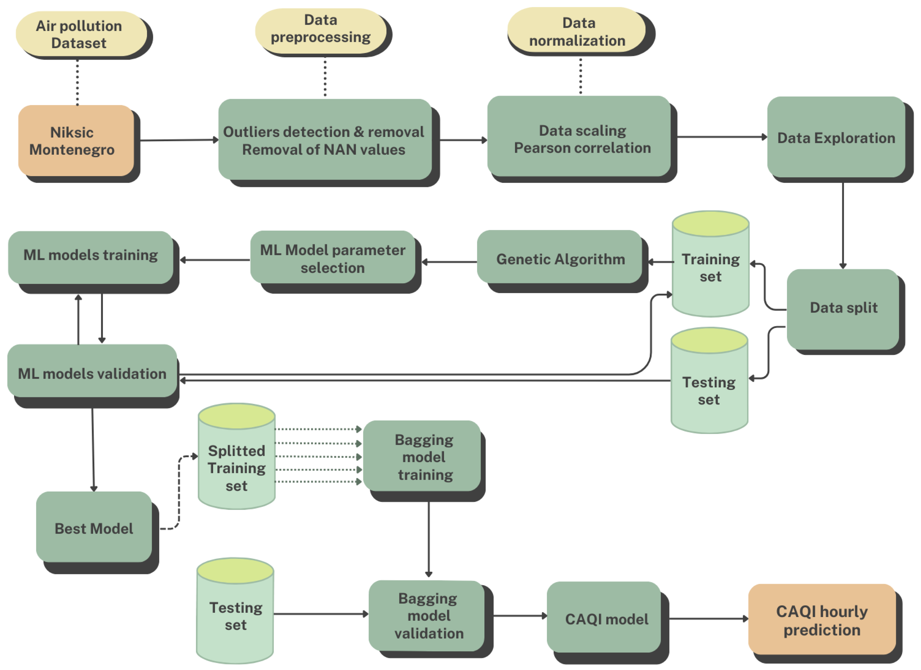
This paper focuses on the hybridization of multiple algorithms. To develop our hybrid model, the Python libraries Keras and Scikit-Learn and their modules $keras.optimizers$ and $sklearn.model\_selection$ were used, as well as the necessary functions and algorithms contained in these modules. A comprehensive description of the proposed system architecture is represented in Figure 1. The various phases employed to obtain hourly air pollution predictions in Niksic, Montenegro are presented. The first step involves collecting air quality data from an air monitoring station. The collected data undergo preprocessing and feature engineering procedures to ensure better training and testing results. After this, the data are partitioned, scaled, and fed into the proposed hybrid LSTM model for further analysis and prediction. In order to enhance the performance of the LSTM model, a GA is employed for parameter selection. This hybridization with the metaheuristic algorithm helps to find the best combination of hyperparameters for LSTM, resulting in the improved predictive capabilities of the model. The bagging technique is applied to the best-performing LSTM model. This approach involves training multiple instances of the LSTM model on distinct subsets of the data and combining their predictions, leading to improved overall accuracy and robustness. Based on its predictive performance, the implemented hybrid LSTM model is thoroughly tested and compared with the SVM approach. These two final models are evaluated and analyzed to provide insights into their suitability for air quality prediction.

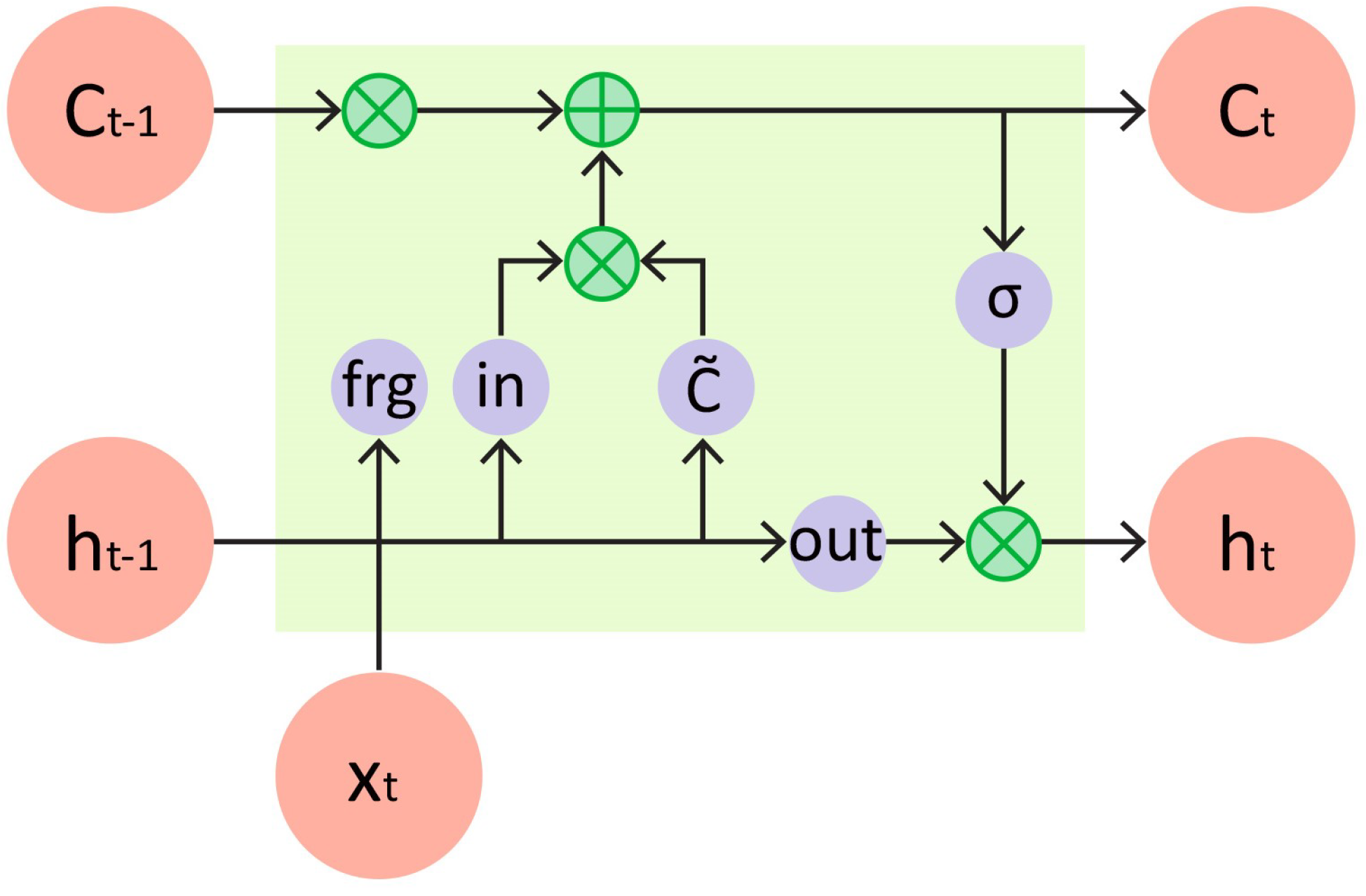
The LSTM algorithm is a type of RNN architecture specifically designed to handle sequential data and effectively capture long-term dependencies [21]. LSTM networks use specialized memory cells and gates to effectively manage and control the flow of information at various time steps. This enables them to effectively model and retain important patterns and dependencies in the input data. The LSTM algorithm addresses the vanishing gradient problem that occurs in RNN algorithms, where gradients become too small to update weights effectively over long sequences. By using memory cells and gates, LSTM allows gradients to flow through time more easily. Figure 2 illustrates the architecture of the LSTM unit, while the corresponding Equations (1)–(6) for the LSTM algorithm are provided below:

$$i{n}_t=\sigma (V_{in}{x}_t+{\omega }_{in}{h}_{t-1}+{\beta }_{in}),$$

(1)

$$fr{g}_t=\sigma (V_{frg}{x}_t+{\omega }_{frg}{h}_{t-1}+{\beta }_{frg}),$$

(2)

$$ou{t}_t=\sigma (V_{out}{x}_t+{\omega }_{out}{h}_{t-1}+{\beta }_{out}),$$

(3)

$${\tilde{\mathcal{C}}}_t=tanh(V_c{x}_t+{\omega }_c{h}_{t-1}+{\beta }_c),$$

(4)

$${\mathcal{C}}_t=fr{g}_t\otimes {\mathcal{C}}_{t-1}+i{n}_{t-1}\otimes {\tilde{\mathcal{C}}}_t,$$

(5)

$$h_t=ou{t}_t\otimes tanh\left({\mathcal{C}}_{t-1}\right),$$

(6)

where the input gate ($i{n}_t$), forget gate ($fr{g}_t$), and output gate ($ou{t}_t$) are controlled by the weights ($V_{in}$, $V_{frg}$, $V_{out}$) connecting them to the input. The weights (${\omega }_{in}$, ${\omega }_{frg}$, ${\omega }_{out}$) connect the input, forget, and output gates to the hidden layer. The bias vectors (${\beta }_{in}$, ${\beta }_{frg}$, ${\beta }_{out}$) are associated with the input, forget, and output gates, respectively. The state of the cell at the previous time point is denoted by ${\tilde{\mathcal{C}}}_t$ and the current state of the cell by ${\mathcal{C}}_t$. The outputs of the cell at the previous and current time points are denoted by $h_{t-1}$ and $h_t$, respectively [22].

The GA is an evolutionary-based metaheuristic algorithm that employs the principles of natural adaptation and selective breeding [8]. It operates on a population of individuals, where each individual represents a potential solution to a specific problem. These individuals are characterized by a genetic code, which is a sequence of characters (genes) from some alphabet. By decoding each individual and assessing its fitness value, the algorithm determines the quality of solutions within the population. Through iterative processes of selection, crossover, and mutation, the GA seeks to optimize the solutions until a specific stopping criterion is met. This criterion can be a fixed number of generations or a condition where the algorithm terminates if there is no improvement in the best individual over a defined number of generations.

The SVM algorithm belongs to the class of well-known supervised ML algorithms. It shows good performance when it is required to fit functions to the training data and at the same time to minimize produced errors. To handle the demanding relationships between the input features and the target variable, and to ensure the detection of linear decision boundaries, SVM incorporates kernel functions, allowing the mapping of the input data into a multidimensional feature space. The optimization process in SVM involves minimizing the loss function, which consists of a margin violation error and a regularization term [23]. The regularization term maintains a trade-off between the complexity of the model and the training error, thus mitigating the risk of overfitting. The SVM function is defined by Equation (7):

$$f\left(x_i\right)=v\phi \left(x_i\right)+\beta ,$$

(7)

where $\phi \left(x_i\right)$ describes the non-linear mapping function, $x_i$ represents the input vector, and $z_i$ represents the corresponding target value. The values v and $\beta$ are the weight factor and bias, respectively [24]. The estimation of the parameters w and b is achieved through the minimization of the regularized risk function $\rho \left(v\right)$, as denoted by Equation (8):

$$\rho \left(v\right)={\displaystyle \frac{1}{2}}{\parallel v\parallel }^2+P\sum _{i=1}^n{\mathcal{L}}_e(z_i,f\left(x_i\right)).$$

(8)

The regularization term $\frac{1}{2}{\parallel v\parallel }^2$ balances the trade-off between the empirical risk and model flatness. The penalty coefficient P determines the extent of this trade-off. The e-insensitive loss function ${\mathcal{L}}_e(z_i,f\left(x_i\right))$ is defined by Equation (9) and is used to handle errors within a tolerance level e:

$${\mathcal{L}}_e(z_i,f\left(x_i\right))=max\left\{0,|z_i-f\left(x_i\right)|-e\right\}.$$

(9)

If the predicted value falls within the threshold, its contribution to the loss function will be ignored. However, if the predicted value exceeds the threshold, the loss function will take on a value greater than e. To measure the distance between the actual values and the corresponding boundary values of the e-tube, two positive slack variables, $\delta$ and ${\delta }^{*}$, are introduced. This transformation results in the constrained form of Equation (8),

$$minf(v,\delta ,{\delta }^{*})={\displaystyle \frac{1}{2}}{\parallel v\parallel }^2+P\sum _{i=1}^n(\delta +{\delta }^{*}),$$

subject to

$$\left\{\begin{array}{cc}{z}_i-v\phi \left(x_i\right)-\beta \le e+\delta ,\hfill & \delta \ge 0\hfill \\ v\phi \left(x_i\right)+\beta -z_i\le e+{\delta }^{*},\hfill & {\delta }^{*}\ge 0.\hfill \end{array}\right.$$

(10)

The Lagrangian function, defined by Equation (11), is used to solve the previously defined optimization problem (10),

$$\begin{array}{cc}\hfill maxF({\lambda }_i,{\lambda }_i^{*})=& -{\displaystyle \frac{1}{2}}\sum _{i=1}^n\sum _{j=1}^n({\lambda }_i-{\lambda }_i^{*})({\lambda }_j-{\lambda }_j^{*})\kappa (x_i,x_j)\hfill \\ \hfill & +\sum _{i=1}^n{z}_i({\lambda }_i-{\lambda }_i^{*})-e\sum _{i=1}^n{z}_i({\lambda }_i+{\lambda }_i^{*})\hfill \end{array}$$

subject to

$$\sum _{i=1}^n{\lambda }_i-{\lambda }_i^{*}=0,{\lambda }_i,{\lambda }_i^{*}\in \left[0,P\right].$$

(11)

Equation (12) describes the method of calculating the regression function $f\left(x\right)$,

$$f\left(x\right)=\sum _{i=1}^n({\lambda }_i-{\lambda }_i^{*})\kappa (x_i,x_j)+\beta ,$$

(12)

where the Lagrangian multipliers satisfy the constraints ${\lambda }_i\ge 0$ and ${\lambda }_i^{*}\ge 0$. The kernel function $\kappa (x_i,x_j)$ allows for the non-linear mapping of the original data into a higher-dimensional feature space.

3.1. Data Collection and Preprocessing

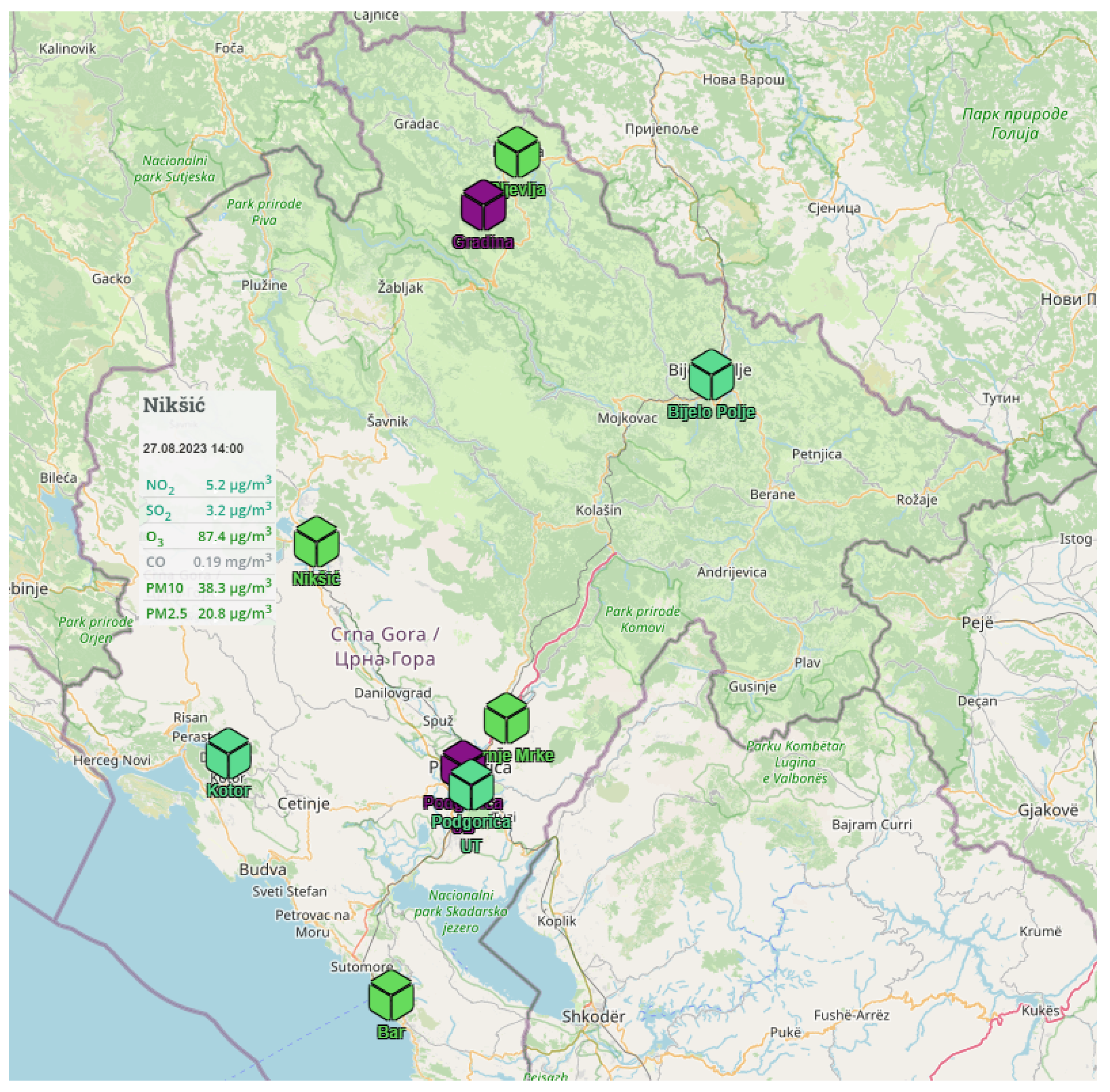
In the analysis described in this paper, data were provided by the Environmental Protection Agency (EPA) of Montenegro. The data were collected from the air quality monitoring station located in Niksic, Montenegro and are freely downloadable from the EPA website [25]. There are 9 monitoring stations in Montenegro, located in Podgorica UT, Podgorica UB, Niksic, Bar, Pljevlja, Bijelo Polje, Kotor, Gornje Mrke, and Gradina, as shown in Figure 3. The focus of the analysis was Niksic, since this town is recognized as one of Montenegro’s urban areas that consistently experiences high pollution levels throughout the year. Our selection was additionally guided by the fact that the datasets obtained from air monitoring stations in other cities in Montenegro were either incomplete or insufficient for our analysis. The air pollutant data from Niksic were recorded from 21 August 2019 until 17 December 2022, and consisted of hourly values of $P{M}_{2.5}$, $P{M}_{10}$, $N{O}_2$, $O_3$, $S{O}_2$, and $CO$.

In general, data collected from monitoring stations, sensors, and other sources cannot be readily utilized for analysis without undergoing necessary preparatory steps. The raw data often contain inconsistencies, outliers, missing values, and other imperfections that need to be addressed. To ensure the accuracy and reliability of subsequent analyses and predictions of our model, multiple preprocessing techniques, including data cleaning, data scaling, and the removal of NAN values, were applied to the collected data. Invalid data (missing data) were simply ignored. To unify data on a common scale, we used a MinMax scaler. It works by transforming each feature independently, maintaining the relationships between the features while ensuring that they all fall within the interval $\left[0,1\right]$. For each feature value x, the scaled value $x_{scaled}$ is calculated using Equation (13):

$$x_{scaled}={\displaystyle \frac{x-x_{min}}{x_{max}-x_{min}}}.$$

(13)

The initial dataset had $\mathrm{28,142}$ values, which was reduced to $\mathrm{17,007}$ after missing data elimination. With the outlier detection and removal, the dataset was additionally reduced to $\mathrm{16,913}$ values. As with other ML techniques, our approach also requires a phase of training and testing. The final dataset of $\mathrm{16,890}$ values, which is the number of continuous 24 h time series, was divided into training and testing datasets, with $\mathrm{12,672}$ ($75\%$) and 4218 ($25\%$) data values, respectively.

3.2. Feature Engineering

The CAQI value is based on the measurement of several air pollutants: $P{M}_{2.5}$, $P{M}_{10}$, $N{O}_2$, $O_3$, $O_2$, and $CO$. It provides a numerical value or color-coded scale that corresponds to the air quality level, i.e., very low, low, medium, high, and very high, as shown in

Table 1. CAQI scale representation. Concentrations of all pollutants are presented in μg/m³.

CAQI Scale	Index	${\mathit{PM}}_{2.5}$ (1 h)	${\mathit{PM}}_{2.5}$ (24 h)	${\mathit{PM}}_{10}$ (1 h)	${\mathit{PM}}_{10}$ (24 h)	${\mathit{NO}}_2$	${\mathit{O}}_3$	${\mathit{SO}}_2$	$\mathit{CO}$
Very low	0–25	0–15	0–10	0–25	0–15	0–50	0–60	0-50	0–5000
Low	25–50	15–30	10–20	25–50	15–30	50–100	60–120	50–100	5000–7500
Medium	50–75	30–55	20–30	50–90	30–50	100–200	120–180	100–350	7500–10,000
High	75–100	55–110	30–60	90–180	50–100	200–400	180–240	350–500	10,000–20,000
Very high	>100	>110	>60	>180	>100	>400	>240	>500	>20,000

.

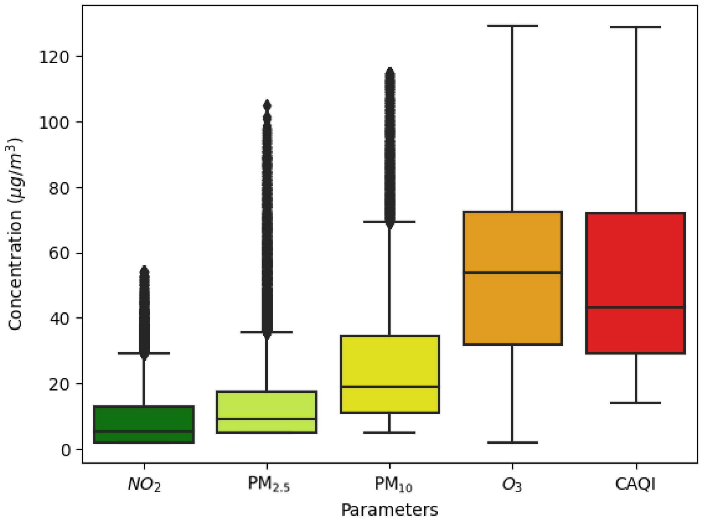
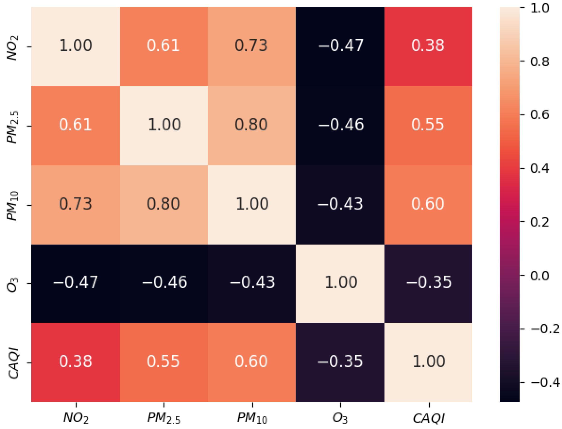
CAQI values are not available on the Montenegro EPA website; only the specific pollutant concentration values are provided, such as $P{M}_{2.5}$, $P{M}_{10}$, $N{O}_2$, $O_3$, $S{O}_2$, and $CO$. Based on the preliminary statistical analysis, 4 pollutants were selected: $P{M}_{2.5}$, $P{M}_{10}$, $N{O}_2$, and $O_3$. The selected pollutants were considered to be equally harmful. Consequently, their weighted factors were set to 1. Due to the low statistical significance, $S{O}_2$ and $CO$ were excluded from further analysis.

The CAQI values were calculated by applying Equation (14) to the 4 selected input parameters:

$$CAQI=max\left\{I_{O_3},I_{P{M}_{2.5}},I_{P{M}_{10}},I_{N{O}_2}\right\},$$

(14)

where the pollutant concentration $\left(C_i\right)$ is mapped to pollutant index $\left(I_i\right)$ by applying the following equation:

$$I_i=I_{low}+{\displaystyle \frac{C_i-C_{low}}{C_{high}-C_{low}}}(I_{high}-I_{low}),$$

(15)

where i denotes the air pollutant. Values $C_{low}$ and $C_{high}$ denote the minimal and maximal 1-h concentration values of the CAQI category that corresponds to the concentration of the specific pollutant, while $I_{low}$ and $I_{high}$ denote the minimal and maximal air quality index values of the category shown in the second column of Table 1. The following calculations are used in our work: maximum mean hourly values for $N{O}_2$, $O_3$ (in μg/m³) and calculated daily mean value for $P{M}_{10}$, $P{M}_{2.5}$ (in μg/m³).

In addition, based on the EPA recommendation, in order for the measurement to be considered valid, it is necessary that there are at least three measured values of the input parameters at the same time, and that among them there is at least one measured value for $N{O}_2$, $P{M}_{10}$, or $O_3$, which we also took into account.

As an example, based on the CAQI system provided by the Montenegro EPA website [4], if the concentration of $P{M}_{10}$ is $C_{P{M}_{10}}$= 82.2 μg/m³, it will fall within the concentration interval of 50 and 90 and the index interval of 50 and 75, corresponding to a moderate pollutant level. The index value $I_{P{M}_{10}}$ is then calculated based on Equation (15) as follows:

$$I_{P{M}_{10}}=50+{\displaystyle \frac{82.2-50}{90-50}}(75-50)=70.125,$$

(16)

It is important to note that, while one pollutant may have the highest concentration value, another pollutant could be dominant, meaning it has the highest index value. This ambiguity comes from different concentrations of certain input quantities that are considered dangerous.

3.3. Performance Evaluation

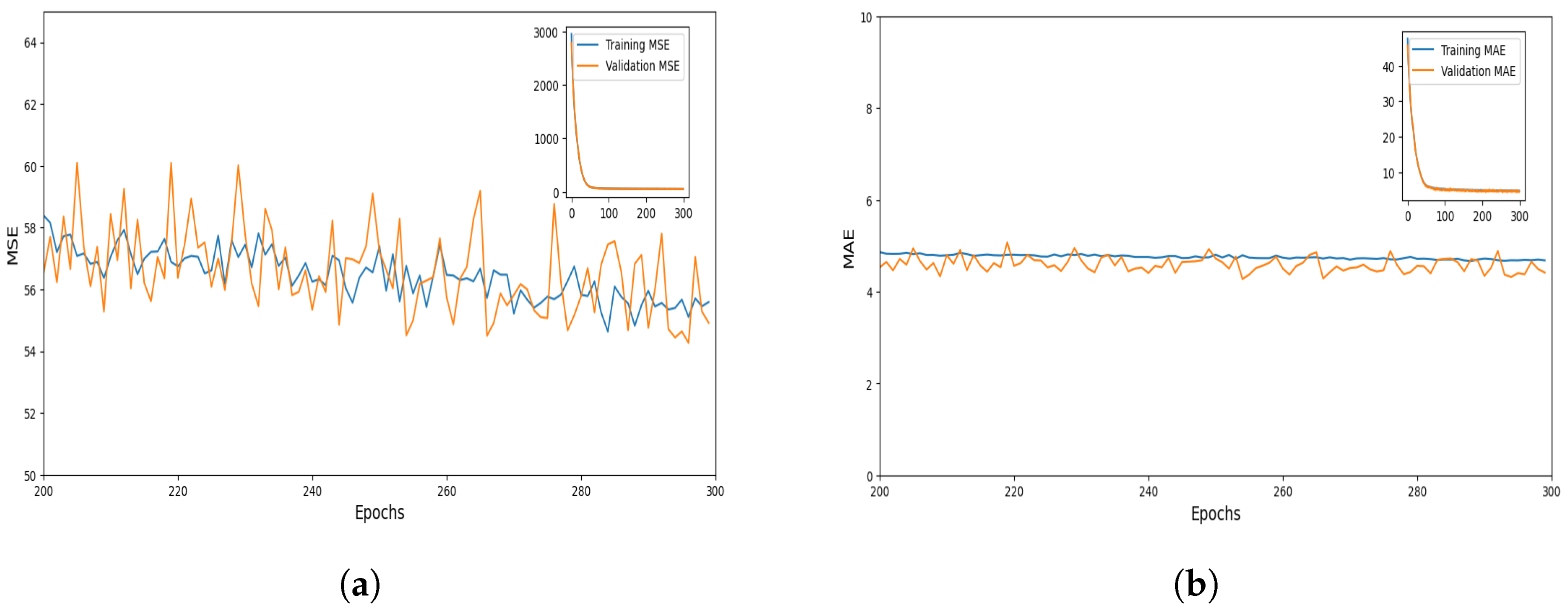
In order to provide a baseline for comparative analysis and to assess the proposed model’s performance, four standard evaluation metrics were applied: Mean Square Error (MSE), Mean Absolute Error (MAE), Mean Absolute Percentage Error (MAPE), and Coefficient of Determination $R^2$.

MSE is a measure used to quantify the extent of deviation between the predicted values (${\widehat{z}}_i$) and measured values ($z_i$). A lower MSE value indicates a smaller deviation. The MSE value is computed using Equation (17):

$$MSE={\displaystyle \frac{1}{n}}\sum _{i=1}^n{\left(z_i-{\widehat{z}}_i\right)}^2.$$

(17)

MAE measures the extent of error between the predicted value and the measured value. The MAE value can be obtained by Equation (18):

$$MAE={\displaystyle \frac{1}{n}}\sum _{i=1}^n|z_i-{\widehat{z}}_i|.$$

(18)

MAPE quantifies the error between the predicted and measured values as a percentage of the measured values. The MAPE value is computed based on Equation (19):

$$MAPE={\displaystyle \frac{1}{n}}\sum _{i=1}^n\left|{\displaystyle \frac{z_i-{\widehat{z}}_i}{{\widehat{z}}_i}}\right|100\%.$$

(19)

The $R^2$ measure indicates how well the air pollutant values in a regression model explain the variation in the CAQI value. It quantifies the proportion of the total variation in the CAQI values that can be accounted for by the air pollutants. The $R^2$ value ranges from 0 to 1, and a higher $R^2$ value indicates a better fit, meaning that a larger proportion of the variation in the CAQI values is captured by the air pollutants. The $R^2$ measure is calculated as shown in Equation (20):

$$R^2=1-{\displaystyle \frac{{\sum }_{i=1}^n{\left(z_i-{\widehat{z}}_i\right)}^2}{{\sum }_{i=1}^n{\left(z_i-\overline{z}\right)}^2}},$$

(20)

where $\overline{z}$ represents the mean of the measured values and n is the number of samples.

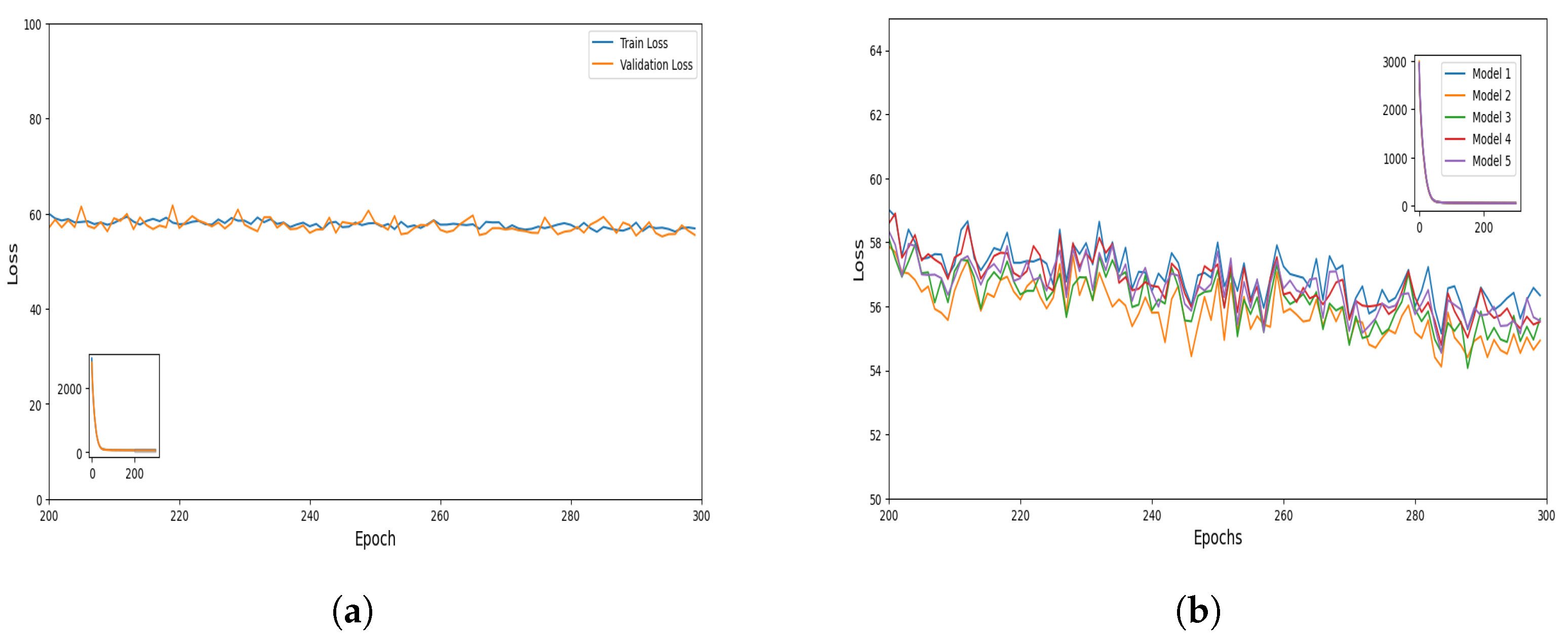
The issue of bias can arise in performance validation when the dataset is split, trained, and tested only once [26]. This implies that the validity of the results obtained from the testing dataset may be affected when the testing subset is altered. To address this problem, each model in our work was rebuilt five times using different random subsets of training and testing samples, while maintaining a consistent splitting proportion of 75:25.

4. Results and Discussion

4.1. Data Summary

After the necessary eliminations and reductions of the initial measurement set, the CAQI values were calculated by applying Equation (14) for the remaining $\mathrm{16,913}$ readings of each pollutant. The descriptive statistics (Count, Mean, Standard Deviation (Std), Minimum (Min), First Quartile (Q1), Median (Q2), Third Quartile (Q3), and Maximum (Max)) of the input dataset are shown in the first column of

Table 2. Descriptive statistics of the dataset.

Metric	${\mathit{NO}}_2$ (μg/m3)	${\mathit{PM}}_{2.5}$ (μg/m3)	${\mathit{PM}}_{10}$ (μg/m3)	${\mathit{O}}_3$ (μg/m3)	CAQI
Count	16,913	16,913	16,913	16,913	16,913
Mean	9.30	16.04	26.78	52.61	51.01
Std	9.74	17.48	22.58	25.69	26.14
Min	2.00	5.00	5.00	2.00	14.00
Q1	2.00	5.00	11.10	31.90	29.00
Q2	5.20	9.00	18.70	53.90	43.00
Q3	12.90	17.20	34.40	72.20	72.00
Max	54.30	104.80	114.90	129.40	129.00

. Columns two to five correspond to the input features of our model and the last column presents the calculated values of CAQI. CAQI represents the output variable that our model aims to predict based on the known input feature concentrations, $O_3$, $P{M}_{2.5}$, $P{M}_{10}$, and $N{O}_2$, displayed in μg/m³.

A concise summary of the dataset is presented with the boxplot displayed in Figure 4. The boxplot illustrates the distribution of concentrations for four pollutants: $P{M}_{2.5}$, $P{M}_{10}$, $N{O}_2$, and $O_3$, and CAQI values. Figure 4 reveals that $P{M}_{2.5}$ and $P{M}_{10}$ exhibit similar distributions, with both pollutants showing positively skewed tendencies. The $P{M}_{2.5}$ interquartile range (IQR) is narrower than the IQR for $P{M}_{10}$, suggesting that $P{M}_{2.5}$ concentrations are relatively less variable. Both pollutants display many outliers, indicating extreme pollution events. The percentage of outliers in $P{M}_{2.5}$ is $11.87\%$ and that in $P{M}_{10}$ is $7.15\%$. The $N{O}_2$ dataset shows a moderately positively skewed distribution with a narrow IQR and the percentage of outliers in $N{O}_2$ is $5.87\%$. The median concentration of $O_3$ indicates a lower central tendency, and there are no outliers in $O_3$. The range of CAQI values is considerably extensive and these values have the greatest dispersion, resulting in a challenge for modeling. Additionally, there are no outliers within the CAQI dataset.

Figure 5 shows the Pearson correlation coefficients between selected air pollutants, $P{M}_{2.5}$, $P{M}_{10}$, $N{O}_2$, $O_3$, and the CAQI values. The strength and direction of the linear correlation between the CAQI values and the measured pollutants are shown as values falling between −1 and $+1$. The correlation coefficient of $0.8$ between $P{M}_{2.5}$ and $P{M}_{10}$ indicates a strong positive correlation between the two pollutants. The correlation coefficient between $P{M}_{2.5}$ and $N{O}_2$ is $0.61$, indicating a moderate positive correlation. On the other hand, the correlation coefficient between $O_3$ and $P{M}_{2.5}$ is $-0.46$, and that between $O_3$ and $N{O}_2$ is $-0.47$, indicating a moderate negative correlation. There is a moderate positive correlation between the CAQI values and $P{M}_{2.5}$ ($0.55$), as well as between the CAQI values and $P{M}_{10}$ ($0.6$). The correlation coefficient between the CAQI values and $O_3$ (−0.35) indicates a moderate negative correlation.

Figure 6 presents the values of four air pollutants ($P{M}_{2.5}$, $P{M}_{10}$, $N{O}_2$, and $O_3$) collected over the 3-year period, together with five CAQI levels. The most frequent CAQI levels in relation to $P{M}_{2.5}$ and $P{M}_{10}$ are high and very high. In relation to $N{O}_2$ and $O_3$, low, medium, and high CAQI levels are equally distributed. In the legends of the plots shown in Figure 6, we provide percentages that describe how many measurements of the parameter shown on the y-axis influenced some of the CAQI levels. For example, a very high level of CAQI was reached due to the maximal $P{M}_{2.5}$ in $0.12\%$ of the data, $69.22\%$ due to the maximal $P{M}_{10}$, and $30.66\%$ of cases due to the maximal $O_3$, while $N{O}_2$ did not cause a very high level of CAQI in any measurement. Observing Figure 6, it is evident that the dataset used is characterized by $14.32\%$ of very low CAQI values, $46.05\%$ of low CAQI values, $16.33\%$ of medium CAQI values, $18.44\%$ of high CAQI values, and $4.86\%$ of very high CAQI values.

In order to gain better insights and visually depict the relationships between the features and the calculated values of CAQI, a pairplot is presented in Figure 7. This allows for a comprehensive visualization of the associations between different variables. The main diagonal of the pairplot represents the distributions of the pollutant concentrations. The concentrations of $N{O}_2$, $P{M}_{2.5}$, and $P{M}_{10}$ show the similarities in their behavior, with heavily rightly skewed tendencies and a narrow spread of values. This indicates the higher concentrations of these pollutants in the dataset. Observing the pairplot, it is evident that there exists a strong positive correlation between $P{M}_{2.5}$ and $P{M}_{10}$, suggesting that an increase in one pollutant is associated with an increase in the other one. There is no obvious relationship among the other pollutants. The color points represented in the scatter plot show different CAQI levels. It is observable from Figure 6 and Figure 7 that very high CAQI values imply higher concentrations of $P{M}_{2.5}$, $P{M}_{10}$, and $N{O}_2$. Conversely, CAQI shows a negative correlation with $O_3$. From Figure 5, Figure 6 and Figure 7 it can be concluded that the concentration levels of $P{M}_{2.5}$, $P{M}_{10}$, and $N{O}_2$ considerably impact the air quality, i.e., the CAQI levels.

4.2. CAQI Prediction Model Implementation

The proposed system aims to create advanced hourly air pollution predictions by implementing a hybrid LSTM model. Hybridization in this paper involves the use of the GA, given the advantageous characteristics of this algorithm. The GA metaheuristic is applied to elevate the LSTM’s accuracy and aims to find the best combination of a suitable time step number and the number of LSTM units in each layer. The GA parameter settings are displayed in

Table 3. GA parameter setting.

Parameter	Value
Crossover probability	0.9
Number of generations	4
Mutation probability	0.3
Population size	4
Fitness function	MSE

. The fitness function is the same as the MSE of the model produced by each individual. To create the next generation, one-point crossover was performed, with a crossover probability of $0.9$. The selection of individuals was performed using tournament selection, with a tournament size of 3. Mutation was applied on the offspring with a mutation probability of $0.3$. The mutation uniformly modified both genes, and it could either increase or decrease the values within the given ranges. In our GA, individuals distinguished by a chromosome composed of two genes represented as integers were used. The first gene determines the number of hidden layers, while the second gene determines the number of time steps. These values are tailored for the effective implementation of the LSTM hybrid model. The values of the first gene (the first parameter) were randomly taken from the interval 7–15 and the values of the second gene (the second parameter) were randomly taken from the interval 24–40. The range of $(24,40)$ was considered for the selection of the optimal number of time steps, while the range of $(7,15)$ was examined to choose the best number of units. Bearing in mind that the GA was used for the LSTM model parameters’ fine-tuning, a GA search was applied to find the most favorable combination of values for the time step and hidden layer size, while other parameters that characterized the GA itself were taken as fixed values and were not subjected to detailed analysis.

The best hyperparameter settings for the LSTM model are presented in

Table 4. LSTM hyperparameter setting.

Hyperparameter	Value
Number of features	4
Number of outputs	1
Number of time steps (selected by GA)	24
Hidden layer size (selected by GA)	15
Batch size	8
Number of epochs	300
Dropout rate	0.2
Recurrent dropout	0.2
Learning rate	0.0001
Optimizer	Adam
Activation	Relu
Number of bags	5

. While there are certain guidelines for the setting of hyperparameters, it is necessary to optimize them as their values rely on the quality of the data. The chosen set of hyperparameters affect the ML algorithm’s performance, especially the CPU time necessary for training and testing and the memory usage to store model and intermediate results. In the literature [11], it has been demonstrated that taking a relatively small number of time steps is sufficient to obtain good performance of the algorithm. The time step value is related to the number of time steps in the input sequences used to train the LSTM model. The input data to the LSTM model are organized into value sequences, each containing 24 consecutive observations, and the LSTM model processes these sequences to learn patterns and relationships in the data over time. During training, the input data are divided into sets of 24 consecutive observations. The model takes these sequences as input and is trained to predict the next value in the sequence (i.e., the 25th observation) as an output. In essence, the model learns the relationships between an input string and the individual output value that follows it. The choice of 24 time steps as the lower bound of the interval was made based on the assumption that CAQI values exhibit relatively periodic changes, considering daily human activity. However, larger values were also allowed, considering the tendency shown by numerical results addressing similar issues. By increasing the upper bounds of the intervals, we enabled the model to better learn patterns from the dataset. It was found that the best accuracy and convergence were achieved for 15 hidden units in the LSTM layer and 24 time steps. Preliminary tests showed that Adam demonstrated the best performance among all observed optimizers. The training model was configured with a total of 300 epochs and a batch size of 8.

The performance of the best LSTM model with applied GA for hyperparameter tuning was evaluated using the MSE, MAE, MAPE, and $R^2$ evaluation metrics, as shown in the third column of

Table 5. SVM, best LSTM, and ensemble model evaluation results in hourly CAQI prediction.

Performance Metric	SVM Model	Best LSTM Model	Ensemble Model
MSE	428.2885	58.8046	56.5810
MAE	13.8739	4.6657	4.5560
MAPE	0.2685	0.0923	0.0912
$R^2$	0.3820	0.9135	0.9168

. The learning curve is displayed in Figure 8a, showing the decreasing trend of the loss function with each epoch. This rapid decline in loss is attributed to the high quality of the model and the well-tuned model parameters. The convergence graph for the five models in the bagging ensemble is shown in Figure 8b. The training and testing MSE and MAE history for the ensemble model with bagging are presented in Figure 9.

The performance of the ensemble model with bagging was evaluated using four evaluation metrics, as presented in the fourth column of Table 5. The actual and predicted values on a subset of the test dataset for the ensemble model with bagging are displayed in Figure 10.

In our analysis, the performance difference between the LSTM model and the ensemble model was assessed, revealing a reduced MSE difference value of −9.3688, indicating improved algorithm performance in terms of lower error and better prediction. As a result, the quality of the model was increased. The performance difference between the best LSTM model without bagging and the ensemble model was also assessed, resulting in an MSE difference of −2.2236 (see

Table 6. Best model (without bagging) and ensemble model comparison.

Performance Metric Difference	Value
MSE Difference	−2.2236
MAE Difference	−0.1097
MAPE Difference	−0.0010
$R^2$ Difference	0.0033

).

Regarding the SVM model, preliminary tests to adjust its hyperparameters were performed. The best-performing SVM model, which was used for the comparison with the ensemble model with bagging, had the following hyperparameters: the radial basis function was used as the kernel function, the parameter that represented the penalty factor was set to 1, and the regularization parameter was set to 2. This value of the penalty factor enabled the resulting SVM model to be less sensitive to outliers and focus more on the general patterns of the data. Additionally, a relatively large value of the regularization parameter ensured that the model had a wider margin of tolerance for errors. This enabled the comparison between the best-performing SVM model and the ensemble model with bagging.

The performance evaluation of the best-performing SVM model yielded a high value of MSE ($428.2885$) and a low $R^2$ measure ($0.3820$), as shown in the second column of Table 5. These low performance results of the SVM model can also be seen in Figure 11, where the actual and predicted values on a subset of the test dataset for the SVM model are presented. The comparison between the SVM and the ensemble model with bagging yielded an MSE difference of $-371.7075$ and an $R^2$ difference of $0.5348$ (see

Table 7. SVM model and ensemble model comparison.

Performance Metric Difference	Value
MSE Difference	−371.7075
MAE Difference	−9.3180
MAPE Difference	−0.1773
$R^2$ Difference	0.5348

). The actual values and predicted values for the SVM and the ensemble model on a subset of the test dataset are presented in Figure 12. Our model demonstrates improved performance compared to the SVM model. It achieves a more than five-times improvement in terms of MSE, indicating better accuracy in predicting the output variable. There is a $67\%$ reduction in terms of MAE, reflecting the enhanced accuracy of the proposed model. The MAPE is also reduced by a factor of three, indicating more reliable predictions. The $R^2$ value is increased from $0.3820$ to $0.9168$, showing a stronger correlation between the predicted and actual values. These results highlight the superior quality of our ensemble model with bagging compared to standard ML techniques, such as SVM.

4.3. Statistical Analysis

A comparative statistical analysis was conducted on the calculated MAE values obtained from the training and testing of three models: the LSTM model, the best LSTM model without bagging, and the ensemble model with bagging. The summary statistics for the calculated MAE values obtained from the training and testing of the models are presented in

Table 8. Summary statistics for the calculated MAE values obtained from training and testing of the LSTM model, the best LSTM model without bagging, and the ensemble model.

Dataset	Model	Minimum	Maximum	Mean	Std. Deviation
	LSTM	4.909	48.593	8.861	8.2130
MAE training set	Best LSTM without bagging	4.751	47.253	7.186	6.599
	Ensemble model	4.665	47.614	7.112	6.578
	LSTM	4.695	47.434	8.921	8.484
MAE testing set	Best LSTM without bagging	4.410	45.694	7.049	6.636
	Ensemble model	4.274	45.639	6.953	6.610

.

In order to examine whether datasets are following Gaussian distribution the following hypotheses were tested: the null hypothesis ($H_0$) assuming that the data is normally distributed and the alternative hypothesis ($H_a$) assuming that the data is not normally distributed. The Shapiro–Wilk normality test was performed for the calculated MAE values obtained from the training and testing of the models. The test statistics (W) were low, below 1, and the p-values were less than $0.0001$, indicating that the observed data significantly deviated from a normal distribution, as is shown in

Table 9. Shapiro–Wilk test for the calculated MAE values obtained from training and testing of the LSTM model, the best LSTM model without bagging, and the ensemble model.

Dataset	Model	W	p-Value	$\mathit{\alpha }$
	LSTM	0.540	<0.0001	0.05
MAE training set	Best LSTM without bagging	0.400	<0.0001	0.05
	Ensemble model	0.404	<0.0001	0.05
	LSTM	0.547	<0.0001	0.05
MAE testing set	Best LSTM without bagging	0.409	<0.0001	0.05
	Ensemble model	0.412	<0.0001	0.05

. A probability–probability (P-P) plot was generated to illustrate that the calculated MAE values obtained from the training and testing of the three models did not adhere to a normal distribution. As can be seen in Figure 13, the points deviated significantly from the equality line, strongly suggesting that the examined datasets did not follow a normal distribution.

Checking the normality (Shapiro–Wilk test) of the MAE distribution helps in selecting the appropriate statistical tests and in ensuring the validity of the conclusions drawn from these tests. Assuming normality is often a prerequisite for certain parametric tests like ANOVA or t-tests. If the MAE data is normally distributed, it implies that the underlying errors are evenly distributed around the mean error and that the ANOVA test would be appropriate for further statistical analysis. If the MAE data is not normally distributed, tests that do not assume a specific distribution of data (non-parametric tests like the Kruskal–Wallis test) are more appropriate.

We further performed the non-parametric Kruskal–Wallis test [27] with a significance level ($\alpha$) set at $0.05$ and 2 degrees of freedom. This test is employed to compare k samples when dealing with non-Gaussian distributions. The null hypothesis tested whether the samples came from the same population. For the calculated MAE values obtained from the training of the models, the calculated K statistic was $109.245$, while the critical value was $5.991$. The calculated two-tailed p-value was found to be less than $0.0001$, indicating significant differences in the performance of the models under consideration. Consequently, the null hypothesis was rejected with a confidence level exceeding $99.99\%$. In the case of calculated MAE values obtained from the testing of the models, the calculated K statistic was $117.872$, while the critical value was $5.991$. The calculated two-tailed p-value was found to be less than $0.0001$, indicating that the null hypothesis had to be rejected.

To determine which models resulted in the rejection of the null hypothesis, it was essential to conduct multiple pairwise comparison procedures. In this research, we employed the two-tailed Steel–Dwass–Critchlow–Fligner test [28] on the calculated MAE values obtained from the training and testing of the three models. Based on the rank values for the models according to the calculated MAE values obtained from training and testing, as displayed in

Table 10. Multiple pairwise comparisons using the Steel–Dwass–Critchlow–Fligner procedure. Two-tailed test on the calculated MAE values obtained from training and testing of the LSTM model, the best LSTM model without bagging, and the ensemble model.

Dataset	Sample	Sum of Ranks	Mean of Ranks	Groups
	Ensemble model	107,205.000	357.350	A
MAE training set	Best LSTM without bagging	126,283.000	420.943	$B$
	LSTM	171,962.000	573.207	$C$
	Ensemble model	107,352.000	357.840	A
MAE testing set	Best LSTM without bagging	124,245.000	414.150	$B$
	LSTM	173,853.000	579.510	$C$

, the models were categorized into three distinct groups. It is not necessarily the group with the smallest mean of ranks that caused the rejection of the null hypothesis. Since p-values are lower than $0.0001$ (the significance level is $0.05$), we can conclude that all three models are responsible for rejecting the null hypothesis. The groups in the last column indicate that all three algorithms are classified according to their performance into separate units and, if they are compared in pairs, no two algorithms are similar. The first group consisted of the ensemble model exhibiting similar performance, the best LSTM model without bagging was placed in the second group, and the LSTM model was placed in the third.

Finally, the Kolmogorov–Smirnov test was conducted to compare the distribution between the LSTM without bagging and the ensemble model. The null hypothesis assumed that both models had the same distribution. The significance level for this test was set at $\alpha =0.05$. For the calculated MAE values obtained from the training of the models, the resulting D-value statistic was $0.250$ and the p-value was less than $0.0001$, leading to the rejection of the null hypothesis with a risk lower than $0.01\%$. For the calculated MAE values obtained from the testing of the models, the resulting D-value statistic was $0.153$ and the p-value was $0.001$, leading to the rejection of the null hypothesis with a risk lower than $0.15\%$. Hence, for the calculated MAE values obtained from the training and testing of the models, the LSTM model without bagging and the ensemble model exhibited differences in the distribution of their respective values. Based on our comprehensive statistical analysis, it is evident that the ensemble model outperformed the LSTM and the best LSTM model without bagging.

5. Conclusions

Air pollution is a global issue that affects countries and regions around the world. It has wide-ranging impacts on various aspects of the environment, public health, and the global climate system. This problem has been further aggravated due to the increase in the global population, urbanization, industrialization, and climate change. There is an urgent need to provide precise predictions of air pollution levels, which will contribute to improving public health and overall quality of life.

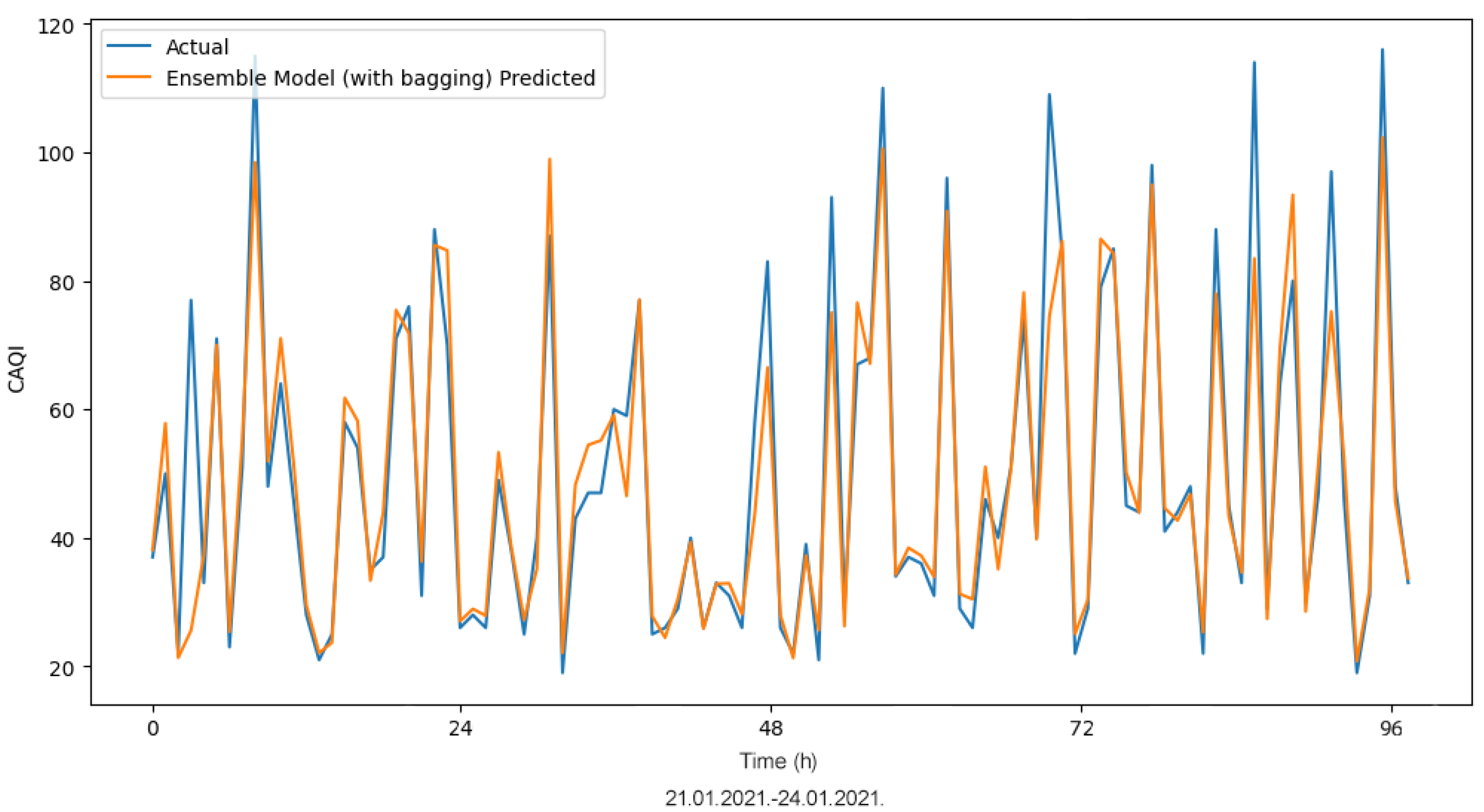
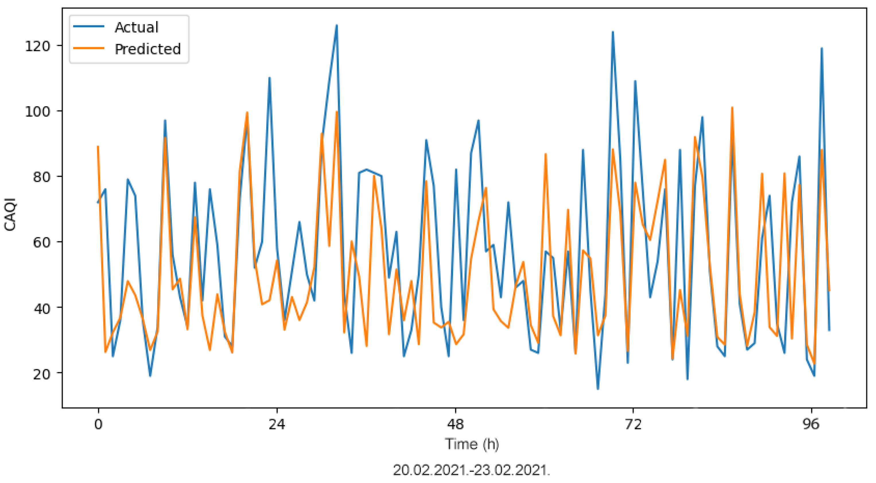
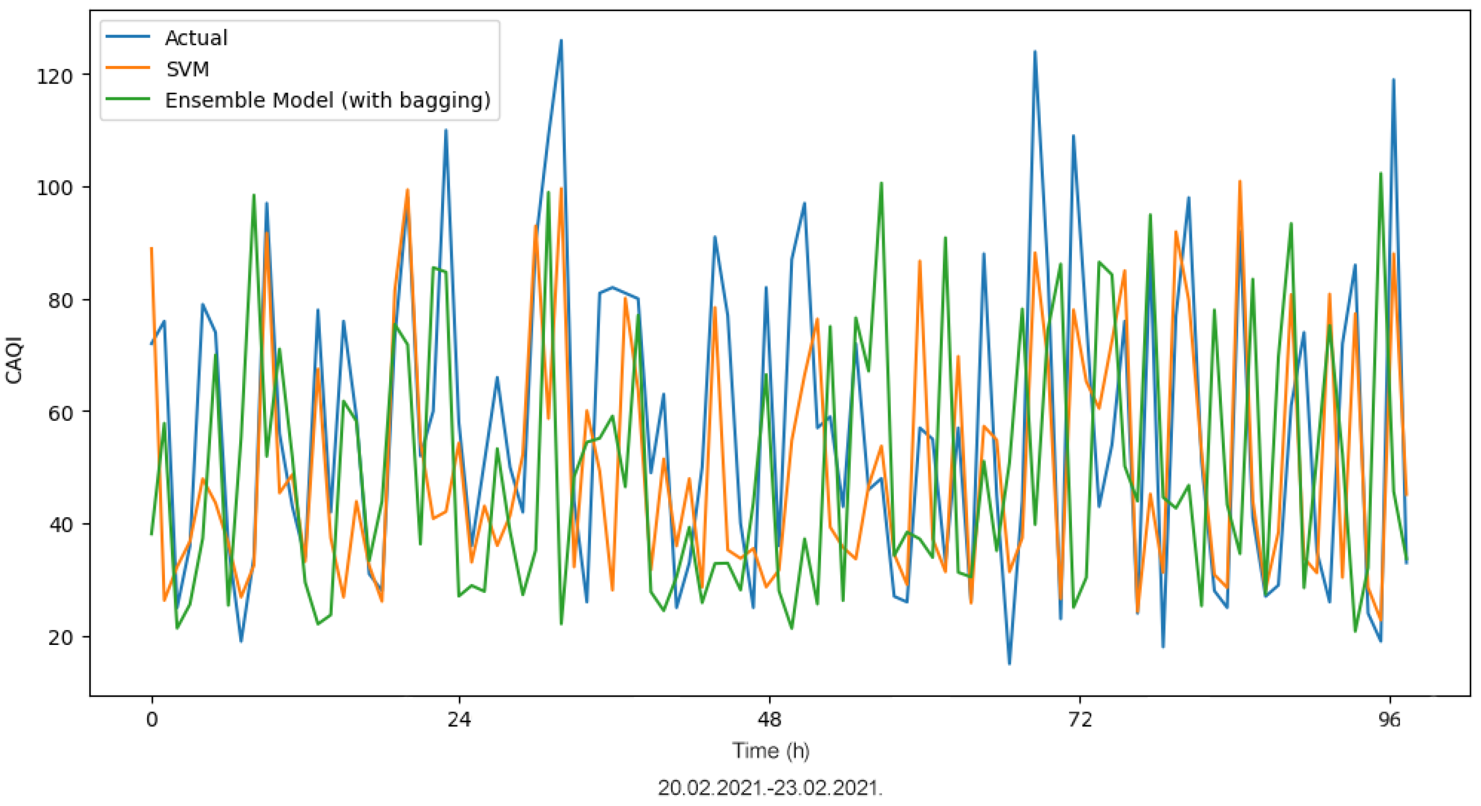
The application of ML algorithms provides promising results for CAQI prediction. The focus of this paper was to propose an advanced hybrid ML model for hourly CAQI prediction in the region of Niksic, Montenegro. The proposed hybrid LSTM model with bagging (i.e., the ensemble model) delivered significantly better performance when compared to the SVM model. A comprehensive statistical analysis was conducted on the calculated MAE values obtained from the training and testing of the LSTM model, the best LSTM model without bagging, and the ensemble model. The results showed that the ensemble model outperformed the other two compared models. This novel hybrid model can be considered as a new and superior alternative for hourly CAQI prediction. The application of such advanced ML analysis using the hybrid approach has not been previously employed in the context of air pollution in Montenegro.

Although our analysis showed that the ensemble model outperformed SVM as a technique to predict CAQI values, we draw the reader’s attention to the fact that SVM is still a promising technique that is worth considering. In particular, it has been shown in the literature that SVM is applicable to CAQI classification problems [29] as well as to regression problems [30], while, in some other papers [31], as in our analysis, SVM has shown slightly worse results. It is evident that the prediction of CAQI values is an extremely complex problem and that the performance of the applied algorithms depends significantly on the characteristics of the dataset; thus, it is important to apply various ML algorithms in modeling, without a priori assumptions that some are inefficient and inapplicable.

The findings of this paper open up several possibilities for future research, such as exploring alternative optimization techniques, incorporating additional variables, considering long-term predictions, conducting comparative studies, and validating the proposed models in different regions, which could contribute to advancing the accuracy and applicability of air quality prediction models. Our future research will also explore the performance of the suggested model in the context of diverse data patterns.

In particular, the potential of other metaheuristic algorithms can be investigated, as well as the hybridization of the existing techniques with additional optimization strategies. Future research could consider incorporating additional variables such as meteorological data (temperature, humidity, wind speed) to enhance the precision and robustness of the predictive models. Predictions with larger time steps, such as 8 h and 24 h predictions, can be considered as well. Further extending the analysis to long-term predictions, such as weekly or monthly forecasts, could provide valuable insights for air quality management and policy planning. Long-term predictions can help to identify patterns, trends, and potential mitigation strategies for sustained improvements in air quality. While this paper compared the performance of the hybrid LSTM, GA, and bagging approach with the SVM model, there may be other ML algorithms or hybrid models that could be included in comparative studies. Assessing the strengths and weaknesses of different models can help to identify the most effective techniques for air pollution prediction. Finally, future works could validate the proposed hybrid model in other regions of Montenegro with varying air pollution characteristics, to assess its transferability and performance in diverse settings.

Monitoring air quality, raising awareness, and implementing effective policies are essential in safeguarding public health and preserving the environment. The proposed model can support efforts to mitigate and reduce air pollution, including the adoption of pollution control measures, the promotion of cleaner energy sources, the improvement of industrial processes, and the adoption of sustainable transportation systems.

References

1. World Health Organization. Air Pollution. Available online: https://www.who.int/health-topics/air-pollution#tab=tab_1/ (accessed on 1 June 2023).
2. van den Elshout, S.; Léger, K.; Nussio, F. Comparing urban air quality in Europe in real time, a review of existing air quality indices and the proposal of a common alternative. Environ. Int. 2008, 34, 720–726. [Google Scholar] [PubMed]
3. van den Elshout, S.; Léger, K.; Heich, H. CAQI Common Air Quality Index–update with PM2.5 and sensitivity analysis. Sci. Total Environ. 2014, 488, 461–468. [Google Scholar] [CrossRef] [PubMed]
4. Environmental Protection Agency of Montenegro. Available online: http://www.epa.org.me/vazduh/caqi (accessed on 1 June 2023).
5. Li, Y.; Sha, Z.; Tang, A.; Goulding, K.; Liu, X. The application of machine learning to air pollution research: A bibliometric analysis. Ecotoxicol. Environ. Saf. 2023, 257, 114911. [Google Scholar] [CrossRef] [PubMed]
6. Wang, W.; Men, C.; Lu, W. Online prediction model based on support vector machine. Neurocomputing 2008, 71, 550–558. Available online: https://www.sciencedirect.com/science/article/abs/pii/S0925231207002883 (accessed on 7 August 2023). [CrossRef]
7. Gul, S.; Khan, G.M. Forecasting Hazard Level of Air Pollutants Using LSTM’s. Artif. Intell. Appl. Innov. 2020, 584, 143–153. [Google Scholar] [CrossRef]
8. Reeves, C.R. Genetic algorithms. In Handbook of Metaheuristics; Gendreau, M., Potvin, J.Y., Eds.; Springer: Berlin/Heidelberg, Germany, 2010; pp. 109–139. [Google Scholar]
9. Eiben, A.E.; Smith, J.E. Introduction to Evolutionary Computing, 2nd ed.; Springer: Berlin/Heidelberg, Germany, 2015. [Google Scholar]
10. Breiman, L. Bagging predictors. Mach. Learn. 1996, 24, 123–140. [Google Scholar] [CrossRef]
11. Drewil, G.; Al-Bahadili, R. Air pollution prediction using LSTM deep learning and metaheuristics algorithms. Meas. Sensors 2022, 10, 100546. [Google Scholar] [CrossRef]
12. Waseem, K.H.; Mushtaq, H.; Abid, F.; Abu-Mahfouz, A.M.; Shaikh, A.; Turan, M.; Rasheed, J. Forecasting of Air Quality Using an Optimized Recurrent Neural Network. Processes 2022, 10, 2117. [Google Scholar] [CrossRef]
13. Xayasouk, T.; Lee, H.; Lee, G. Air Pollution Prediction Using Long Short-Term Memory (LSTM) and Deep Autoencoder (DAE) Models. Sustainability 2020, 12, 2570. [Google Scholar] [CrossRef]
14. Triana, D.; Osowski, S. Bagging and boosting techniques in prediction of particulate matters. Bull. Pol. Acad. Sci. 2020, 68, 1207–1215. [Google Scholar]
15. Liang, Y.-C.; Maimury, Y.; Chen, A.H.-L.; Juarez, J.R.C. Machine Learning-Based Prediction of Air Quality. Appl. Sci. 2020, 10, 9151. [Google Scholar] [CrossRef]
16. Madhuri, V.M.; Samyama, G.H.; Kamalapurkar, S. Air pollution prediction using machine learning supervised learning approach. Int. J. Sci. Technol. Res. 2020, 9, 118–123. [Google Scholar]
17. Kumar, K.; Pande, B.P. Air pollution prediction with machine learning: A case study of Indian cities. Int. J. Environ. Sci. Technol. 2023, 20, 5333–5348. [Google Scholar] [CrossRef]
18. Sanjeev, D. Implementation of machine learning algorithms for analysis and prediction of air quality. Int. J. Eng. Res. Technol. 2021, 10, 533–538. [Google Scholar]
19. Rybarczyk, Y.; Zalakeviciute, R. Machine Learning Approaches for Outdoor Air Quality Modelling: A Systematic Review. Appl. Sci. 2018, 8, 2570. [Google Scholar] [CrossRef]
20. Méndez, M.; Merayo, M.G.; Núñez, M. Machine learning algorithms to forecast air quality: A survey. Artif. Intell. Rev. 2023, 56, 10031–10066. [Google Scholar] [CrossRef] [PubMed]
21. Hochreiter, S.; Schmidhuber, J. Long short-term memory. Neural Comput. 1997, 9, 1735–1780. [Google Scholar] [CrossRef]
22. Rahimzad, M.; Moghaddam Nia, A.; Zolfonoon, H.; Soltani, J.; Danandeh Mehr, A.; Kwon, H. Performance Comparison of an LSTM-based Deep Learning Model versus Conventional Machine Learning Algorithms for Streamflow Forecasting. Water Resour. Manag. 2021, 35, 4167–4187. [Google Scholar] [CrossRef]
23. Cortes, C.; Golowich, S.E.; Smola, A. Support vector method for function approximation, regression estimation, and signal processing. In Advances in Neural Information Processing Systems; MIT Press: Cambridge, MA, USA, 1997; pp. 281–287. [Google Scholar]
24. Cortes, C.; Vapnik, V. Support-vector networks. Mach. Learn. 1995, 20, 273–297. [Google Scholar] [CrossRef]
25. Environmental Protection Agency of Montenegro. Available online: http://www.epa.org.me/vazduh/arhiv/2 (accessed on 1 June 2023).
26. Varma, S.; Simon, R. Bias in error estimation when using cross-validation for model selection. BMC Bioinform. 2006, 7, 1–8. [Google Scholar] [CrossRef]
27. Smith, M.J. Statistical Analysis Handbook: A Comprehensive Handbook of Statistical Concepts, Techniques and Software Tools; The Winchelsea Press: Winchelsea, UK, 2018. [Google Scholar]
28. Critchlow, E.D.; Fligner, A.M. On distribution-free multiple comparisons in the one-way analysis of variance. Commun. Stat.—Theory Methods 1991, 20, 127–139. [Google Scholar]
29. Kulkarni, M.; Raut, A.; Chavan, S.; Rajule, N.; Pawar, S. Air Quality Monitoring and Prediction using SVM. In Proceedings of the 6th International Conference on Computing, Communication, Control And Automation, ICCUBEA, Pune, India, 26–27 August 2022; pp. 1–4. [Google Scholar]
30. Leong, W.C.; Kelani, R.O.; Ahmad, Z. Prediction of air pollution index (API) using support vector machine (SVM). J. Environ. Chem. Eng. 2020, 8, 103208. [Google Scholar] [CrossRef]
31. Zhoul, L.; Chenl, M.; Ni, Q. A hybrid Prophet-LSTM Model for Prediction of Air Quality Index. In Proceedings of the IEEE Symposium Series on Computational Intelligence, Canberra, ACT, Australia, 1–4 December 2020; pp. 595–601. [Google Scholar]
Figure 1. Proposed system architecture for hourly CAQI prediction in Montenegro.
Applsci 13 10152 g001
Figure 2. The structure of the memory unit in the LSTM layer.
Applsci 13 10152 g002
Figure 3. Air monitoring stations in Montenegro.
Applsci 13 10152 g003
Figure 4. Summary of the air pollution dataset used.
Applsci 13 10152 g004
Figure 5. Pearson correlation values.
Applsci 13 10152 g005
Figure 6. Scatterplot of four observed features and the calculated CAQI.
Applsci 13 10152 g006
Figure 7. Visual representation of pairwise feature relationships.
Applsci 13 10152 g007
Figure 8. Convergence graphs representing (a) the best LSTM model without bagging, (b) the five models in the bagging ensemble.
Applsci 13 10152 g008
Figure 9. Training and testing performance metric history for the ensemble model with bagging: (a) MSE, (b) MAE.
Applsci 13 10152 g009
Figure 10. Actual and predicted values for the ensemble model with bagging on a subset of the test dataset.
Applsci 13 10152 g010
Figure 11. Actual and predicted values for the SVM model on a subset of the test dataset.
Applsci 13 10152 g011
Figure 12. Actual values, prediction of the SVM model, and prediction of the ensemble model on a subset of the test dataset.
Applsci 13 10152 g012
Figure 13. Probability plot. (a) Calculated MAE values obtained from training of the LSTM model. (b) Calculated MAE values obtained from testing of the LSTM model. (c) Calculated MAE values obtained from training of the best LSTM model without bagging. (d) Calculated MAE values obtained from testing of the best LSTM model without bagging. (e) Calculated MAE values obtained from training of the ensemble model. (f) Calculated MAE values obtained from testing of the ensemble model.
Applsci 13 10152 g013