Deep Representation of EEG Signals Using Spatio-Spectral Feature Images

Abstract

Modern deep neural networks (DNNs) have shown promising results in brain studies involving multi-channel electroencephalogram (EEG) signals. The representations produced by the layers of a DNN trained on EEG signals remain, however, poorly understood. In this paper, we propose an approach to interpret deep representations of EEG signals. Our approach produces spatio-spectral feature images (SSFIs) that encode the EEG input patterns that activate the neurons in each layer of a DNN. We evaluate our approach using the PhyAAt dataset of multi-channel EEG signals for auditory attention. First, we train the same convolutional neural network (CNN) architecture on 25 separate sets of EEG signals from 25 subjects and conduct individual model analysis and inter-subject dependency analysis. Then we generate the SSFI input patterns that activate the layers of each trained CNN. The generated SSFI patterns can identify the main brain regions involved in a given auditory task. Our results show that low-level CNN features focus on larger regions and high-level features focus on smaller regions. In addition, our approach allows us to discern patterns in different frequency bands. Further SSFI saliency analysis reveals common brain regions associated with a specific activity for each subject. Our approach to investigate deep representations using SSFI can be used to enhance our understanding of the brain activity and effectively realize transfer learning.

1. Introduction

Brain–computer interface (BCI) systems are becoming increasingly popular. The ease of recording electroencephlogram (EEG) signals has facilitated devising and launching new BCI systems for day-to-day applications, ranging from medical uses [1] to gaming [2,3]. However, BCI systems that are trained on EEG signals from one subject alone might not perform well when applied to other subjects. This inability to generalize well is commonly ascribed to individual differences in the brain folding structure, which would result in EEG signals that follow different distributions [4]. Consequently, BCI systems might need to be re-trained on each future subject, which requires collecting and processing new EEG data and is a time-consuming activity. Several frameworks that use the principles of transfer learning have been proposed to calibrate pre-trained EEG-based systems, including filter banks [5], adaptive feature extraction [6], transfer component analysis [7], common spatial pattern [8,9,10], regularized covariance matrix [8,11], canonical correlation analysis [12], and convolutional neural networks (CNNs) [13]. The time-consuming nature of the calibration process remains a major obstacle, and hence, strategies have been proposed to reduce the calibration time on new subjects [11,14].

Transfer learning and re-calibration in EEG studies can be improved by identifying suitable invariant features in EEG signals [15], i.e., EEG patterns that are common across subjects. However, unlike conventional data such as images of physical objects, speech signals, or text, raw EEG signals do not offer an obvious choice of interpretable features. Common options to define EEG features include spectral domain approaches [16]. By including EEG signals from multiple recording sites, richer spatio-spectral features that account for the spatial activity of the brain can also be defined, as in [17]. Given a set of existing features, new sets of derived features can be defined by adding further processing stages. Using this angle, the resulting processing pipeline can be seen as a system that produces multiple representations of the input EEG signals. Such processing pipelines can be hand-crafted or learned by training a model of a predefined architecture.

Deep neural networks (DNNs) are trainable processing pipelines and have become a popular machine learning approach in neuroscience and brain studies. Systematic reviews that focus on the application of DNNs to brain studies can be found in [18,19,20,21]. These reviews discuss the main predictive tasks where DNNs are commonly used, examine their internal architecture, and provide a comparison of the performance of different DNN models. An analysis of the reviewed literature reveals that the majority of the existing proposals consider CNN architectures that take as an input one-dimensional data structures, such as temporal EEG segments or spectral domain representations of EEG signals, or two-dimensional data structures, for instance, spectrograms or scalograms. In a limited number of cases, spatio-spectral inputs are considered. For instance, spatio-temporal representations of EEG signals were used as input in [22,23], who used multi-channel EEG signals as the input of their proposed DNN [24].

As processing pipelines, DNNs internally produce multiple representations of their input, which are known as deep representations. A small fraction of the literature reviewed in [18], where DNN approaches were used in brain studies, considered model inspection, which is needed to interpret the sequence of processing stages in a DNN pipeline. For instance, [23,25] analyzed the weights of a DNN trained on EEG signals. Occlusion and activation maximization have also been used, for instance, in [26,27,28,29,30,31]. Specifically, in [26], spectral and spatial information of EEG signals were combined in a three-channel RGB image and used for training a DNN, and deep representations were analyzed. Finally, some studies have used transfer learning approaches based on deep representations for domain adaptation [32,33]. Despite these efforts, deep representations of EEG signals remain poorly understood due to the lack of interpretability. Improving our understanding of EEG deep representations would be useful not only for explaining the decision process of a trained model, but also for effectively realizing transfer learning and in general gaining insight into the mechanisms of the brain. In this paper, we propose an approach for analyzing deep representations of EEG signals. We base our approach on the common assumption that different frequency bands in EEG signals and brain areas are associated with different brain activities. For each deep representation in a DNN, our approach produces a spatio-spectral feature image (SSFI) which is visualized as a topographic map and identifies the brain areas and different frequency bands associated with the target deep representation. We evaluate our approach on DNN models trained on EEG signals from the Physiology of Auditory Attention (PhyAAt) dataset [34] and in addition carry out an inter-subject dependency (ISD) analysis to explore generalized representations across subjects [35,36].

This paper is organized as follows. Section 2 introduces the PhyAAt dataset, which we use to evaluate our proposed approach. In Section 3, we describe the methods used in this paper, which include generation of SSFIs from multi-channel EEG signals, CNN architecture definition and training, deep representation analysis, and ISD analysis. Section 4 presents the results from our analysis, and finally, Section 5 includes the conclusions and a discussion.

2. Dataset

In this study, we use the PhyAAt dataset [34] to evaluate our proposed approach to analyzing deep representations in DNNs. The PhyAAt dataset provides a collection of 14-channel EEG signals recorded from 25 healthy subjects (labelled as S1 to S25) who underwent a total of 144 trials of an auditory attention experiment. Each trial consisted of three tasks. First, participants were presented with an audio message reproduced under different auditory conditions (listening task); afterwards, the participants transcribed the audio message (writing task), and finally, they enjoyed a resting period before the beginning of the following trial (rest task).

The experimental auditory conditions included different levels of background noise, message lengths, and message semanticity, and the transcription of each audio message was used to define an auditory attention score. An Epoc-Emotiv device [37] was used to record 14-channel EEG signals from each participant. Electrodes were arranged following the standard 10–20 EEG electrode placement, the sampling rate was set to 128 Hz, and the average duration of the complete series of trials for a subject was 40 min. Finally, the time periods covering a single task were labeled according to the type of task, the auditory conditions, and the resulting attention score. The required ethical approval for the experiment was acquired.

3. Methods

We evaluate our approach to analyzing deep representations on DNN models trained to solve a ternary classification problem. This ternary classification problem is that of predicting whether a one-second long, 14-channel EEG segment from the PhyAAt dataset was recorded during a listening, a writing, or a resting task. The implemented prediction pipeline consists of two stages, as shown in Figure 1. First, one-second long 14-channel EEG segments are extracted and transformed into SSFI arrays. Then, each SSFI array is used as an input to a trained CNN model, which labels the segment as either listening, writing, or resting.

In this section, we first define SSFI structures and describe the method that we use to generate them from multi-channel EEG signals. Then, we present our chosen CNN architecture and outline how we use the PhyAAt dataset to train and test multiple CNN models and how we carry out our ISD analysis. Our approach to analyzing deep representations in terms of SSFIs is finally described.

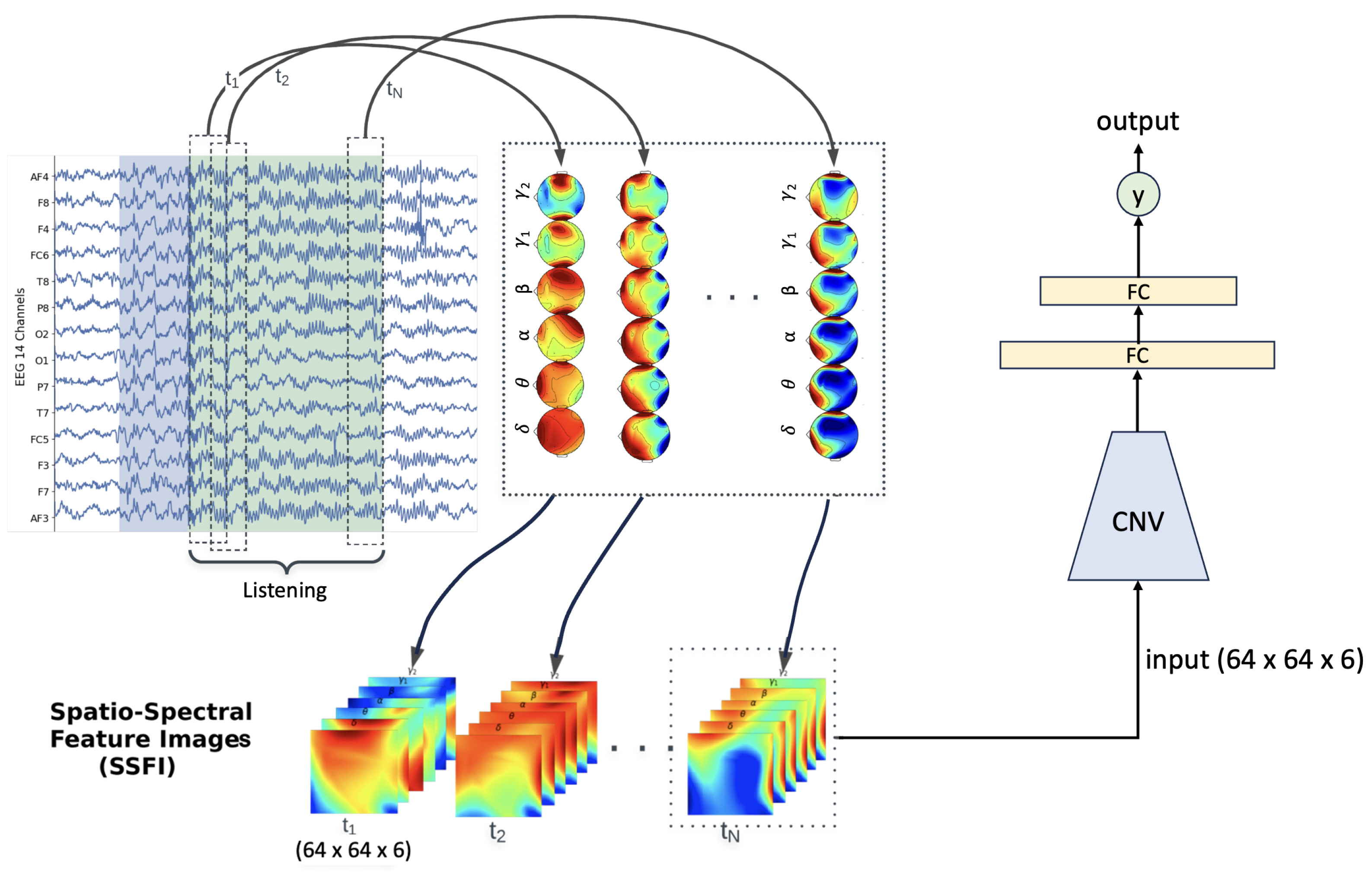
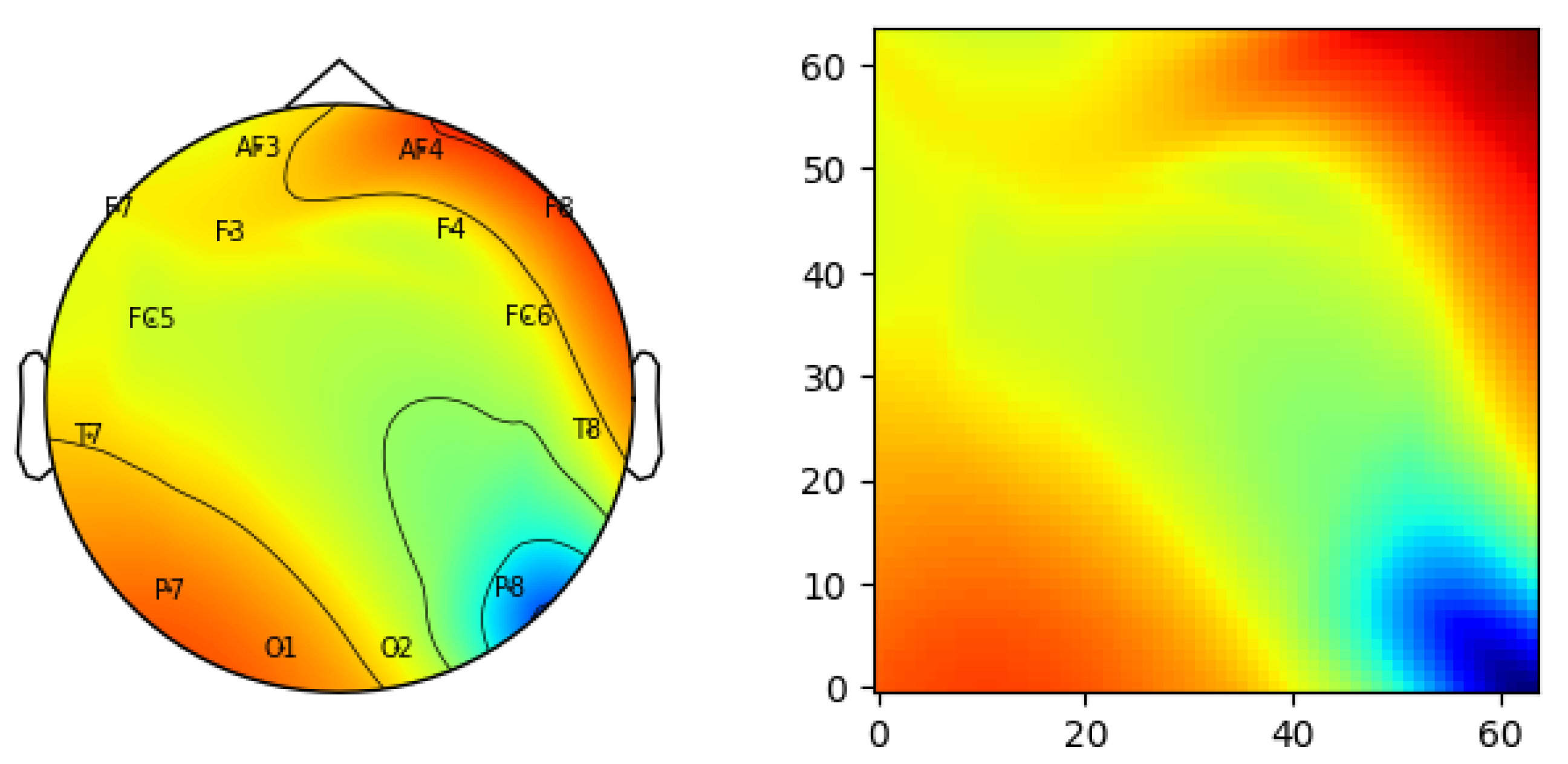
3.1. Spatio-Spectral Feature Image Definition and Generation

An SSFI is a set of images representing EEG data in the spatial and spectral domains. Each image in an SSFI corresponds to a spatio-spectral representation for a single band of frequencies. In EEG studies, there are well-established frequency bands associated with particular mental and emotional states of the brain. Accordingly, in this study, we considered the main EEG frequency bands. Raw 14-channel EEG segments are transformed into SSFI 3D arrays that represent the spatio-spectral distribution of power. The shape of the SSFI 3D array is $D_1\times D_2\times D_3$, where $D_1\times D_2$ is the size of a 2D grid representing the scalp topography and $D_3$ is the number of frequency bands. Preserving the scalp topography is important in multi-channel EEG studies, as spatially close scalp sites are in general affected by common brain sources.

Given a multi-channel EEG segment and a set of $D_3$ frequency bands of interest, an SSFI array is generated as follows. Rectangular grids are used to represent the spatial density of power within one frequency band and are constructed using spherical-to-polar coordinate conversion, so that the scalp locations corresponding to the recording electrodes are associated to one of the grid locations. Based on the power spectral density of each EEG channel, the power in each frequency band is computed and assigned to the electrode’s entry in the corresponding rectangular grid. The spatial density of power on the $D_1\times D_2$ grid is then obtained by interpolating and extrapolating the values computed from each electrode, by using a bicubic method adapted from the MNE library [37]. Figure 2 shows the spatial density of power for a single frequency band on a scalp topography and its corresponding rectangular grid. By stacking the $D_3$ spatial densities of power, we obtain the final SSFI array of dimensions $D_1\times D_2\times D_3$.

Prior to the generation of SSFI arrays, the 14-channel EEG signals were pre-processed as follows. First, each EEG channel was filtered with a fifth-order, highpass IIR filter with cascaded second-order sections and with cut-off frequency of 0.5 Hz. Then, artifacts were removed using the ATAR (automatic and tunable artifact removal) algorithm described in [38], with parameter $\beta =0.1$. After this pre-processing stage, one-second long (128 samples) segments were extracted, allowing 0.75 s (96 samples) overlap (shift 0.25 s, 32 samples) between consecutive segments.

The power spectral density of each segment channel was obtained using the Welch method with a Hamming window. Based on the estimated power spectral density, the power within the following six frequency bands was computed: 0.1–4 Hz (delta, $\delta$), 4–8 Hz (theta, $\theta$), 8–14 Hz (alpha, $\alpha$), 14–30 Hz (beta, $\beta$), 30–47 Hz (low gamma, ${\gamma }_1$), and 47–64 Hz (high gamma, ${\gamma }_2$). This process resulted in a feature vector F of 84 ($6\times 14$) dimensions, $F\in {\mathbb{R}}^{84}$, per EEG segment:

$$F=\left[\begin{array}{c}{F}_{\delta }\\ F_{\theta }\\ F_{\alpha }\\ F_{\beta }\\ F_{{\gamma }_1}\\ F_{{\gamma }_2}\end{array}\right]$$

(1)

where $F_i\in {\mathbb{R}}^{14}$ is the power of the 14 channels of an EEG segment within each band $i\in \{\delta ,\theta ,\alpha ,\beta ,{\gamma }_1,{\gamma }_2\}$. A $64\times 64$ rectangular grid was chosen for the scalp topography, resulting in a $64\times 64\times 6$ SSFI array. Figure 1 illustrates the process of extracting a sequence of SSFI arrays from consecutive 14-channel EEG segments from the PhyAAt dataset.

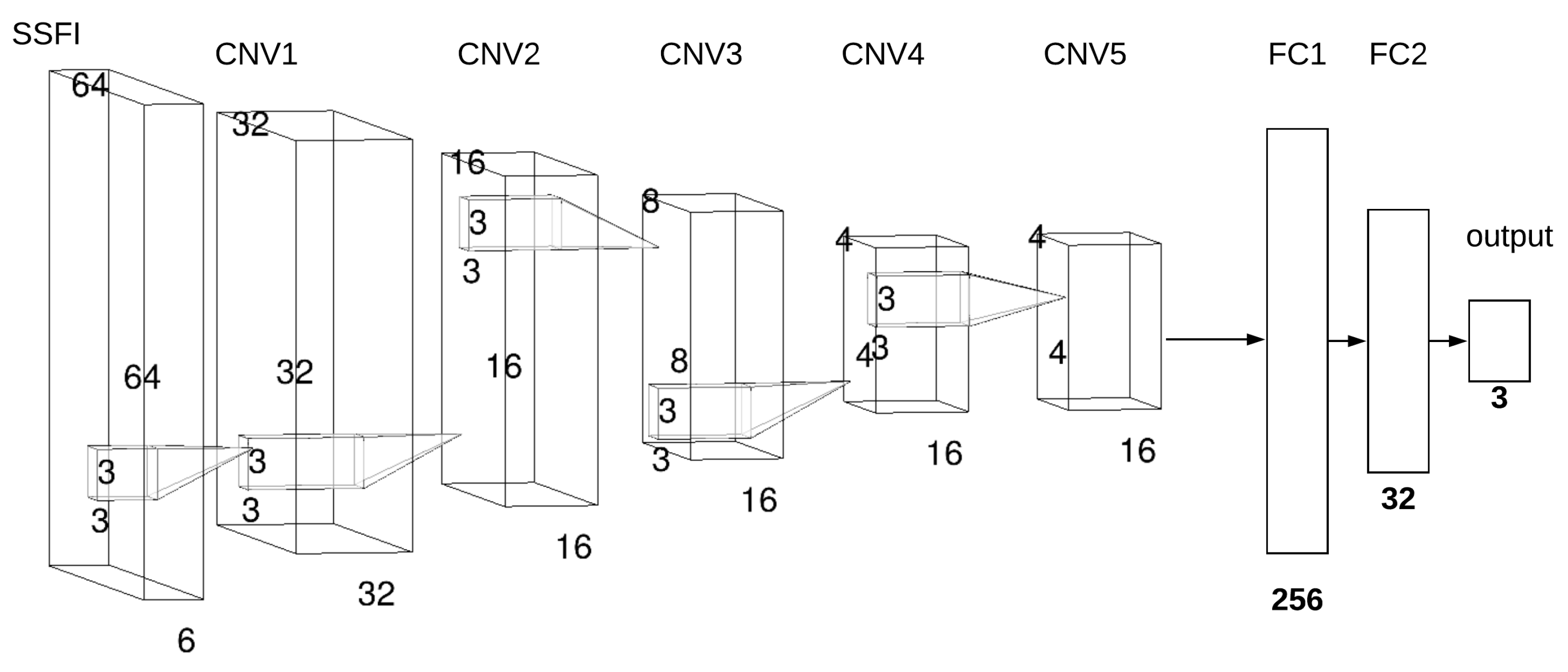
3.2. Neural Network Architecture, Training, and Test

A CNN architecture (Figure 3), consisting of five convolutional layers (CNV), two fully connected layers (FC), and one output layer with three output units, was used to solve the proposed ternary classification problem. The number of input channels in this architecture is six, which corresponds to the number of frequency bands in the input SSFI arrays. Each convolutional layer consists of a bank of filters of size $3\times 3$. The first four convolutional layers are followed by a $2\times 2$ max-pool layer, batch normalization, and dropout ($0.3$) layer. As shown in Figure 3, the first layer (CNV1) has 32 filters and the remaining CNV layers have 16. The activation function used for the output layer is softmax, whereas for the hidden layers, it is a rectified linear unit (ReLu) with $l_2=0.01$ regularization parameter. Dropout and L2 regularization are used to reduce the risk of over-fitting.

Since individual differences in the brain folding structures can result in participants producing different EEG distributions [4], we took a subject-specific approach and trained the proposed CNN architecture on each of the 25 participants separately, which resulted in 25 trained CNN models. In creating the training and test sets for each subject, we took into consideration the existing overlap between consecutive EEG segments, as it can potentially lead to information leak from the training to the test stage. For each subject, the EEG segments corresponding to the first 100 auditory tasks (first 100 trials) were used for training, whereas the EEG segments extracted from the remaining trials (i.e., 44) were used for evaluating the trained CNN models. This serial split of training and testing is used by taking into consideration the role of time in the design of the experiments in the PhyAAt dataset and to replicate a scenario where a model is trained on past data and evaluated in real-time. We used the classification accuracy to quantify the performance of the resulting CNN models. The categorical cross-entropy was chosen as a loss function during training [39] and the Adam (Adaptive Moment Estimation) method was used during optimization.

In order to understand differences of brain activity for the same task in different individuals, we carried out an ISD analysis. In ISD analysis, a trained model on one subject is tested on all the other subjects. For consistency of comparative results, each trained model is also tested on the data from the same subject, including training and test data (i.e., SSFI from all 144 trials).

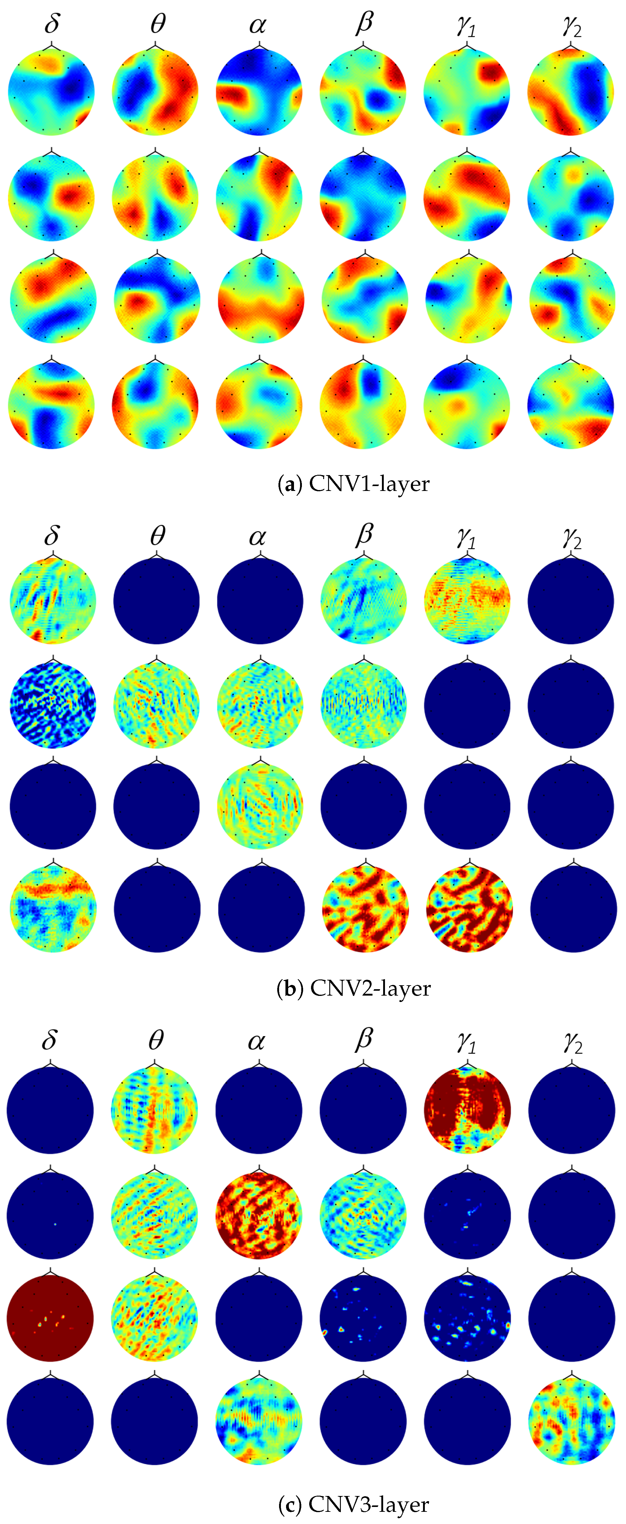
3.3. Deep Representation Analysis

Activation maximization is a common approach to investigating deep representations in DNNs and consists in identifying the input patterns that activate the neurons in each trained layer. The input patterns that activate the neurons in a given layer can be interpreted as those that the layer is focusing on. Therefore, a deep representation can be interpreted in terms of its corresponding maximization patterns. In problems involving images of the natural world, such as faces and objects, this approach produces patterns which can be meaningfully interpreted, such as eyes in a DNN model trained for face recognition, or wheels in a DNN model trained for object recognition. The application of activation maximization to problems involving EEG signals is more challenging, as they lack patterns that posses the interpretability available in images of physical objects, speech signals, or text.

Our approach to analyzing deep representations in a DNN trained on EEG signals produces SSFI patterns. In other words, in our approach, deep representations in a DNN are interpreted by identifying the areas of the brain and the frequency bands that activate the associated layers. We assume that a processing pipeline transforms multi-channel EEG signals into SSFI, which are then fed to a trained DNN, similar to the one presented in Figure 1. Therefore, rather than looking for temporal patterns in EEG signals that activate the layers of a DNN, our approach looks for spatio-spectral patterns. Given a DNN trained on SSFIs, activation maximization patterns are generated by feeding random, noisy images to a trained network and maximizing the activation of a selected deep neuron by updating the input image using the gradient ascent method [40]. Since our input image is not a conventional three-channel RGB image, we display a pattern for each input channel separately. In this study, we train 25 separate CNN models that share the same architecture on SSFI arrays from multi-channel EEG signals from 25 subjects. Comparing the SSFI patterns activating each layer allows us to explore which brain areas and frequency bands are involved in each auditory task for each subject, which can suggest opportunities for transfer learning and shed light into common and individual brain mechanisms.

A second approach to analyzing a trained DNN is to generate saliency maps [41]. In this approach, one of the input images is fed to the DNN, and by computing a gradient, a map is produced that indicates the spatial locations of an input image that are important for computing the output probability score. Saliency maps are usually overlaid on their corresponding input image to identify the areas of the image that are useful in producing the final prediction. Assuming that the input to a DNN consists of SSFIs generated from multi-channel EEG signals, in this study, we create SSFI saliency maps, which identify the brain areas that are relevant for each prediction. Specifically, we focus on those SSFI images from the training set that have the highest probability score for its true class and we generate averaged saliency maps to identify common brain regions that are associated with the listening task.

4. Results

In this section, we first present the performance of the CNN model trained on each subject. Then we use ISD analysis to explore how each model performs on other subjects. Finally, we present the results of the deep representation analysis.

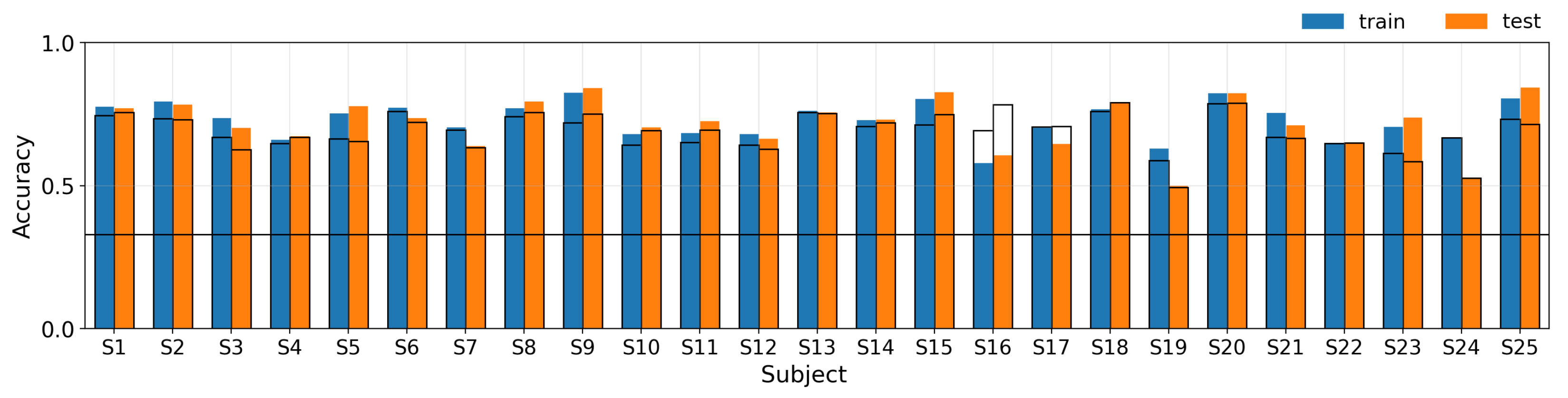
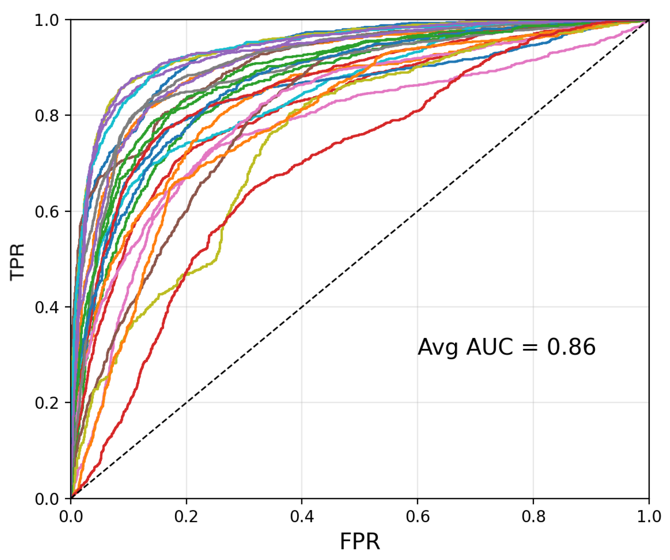
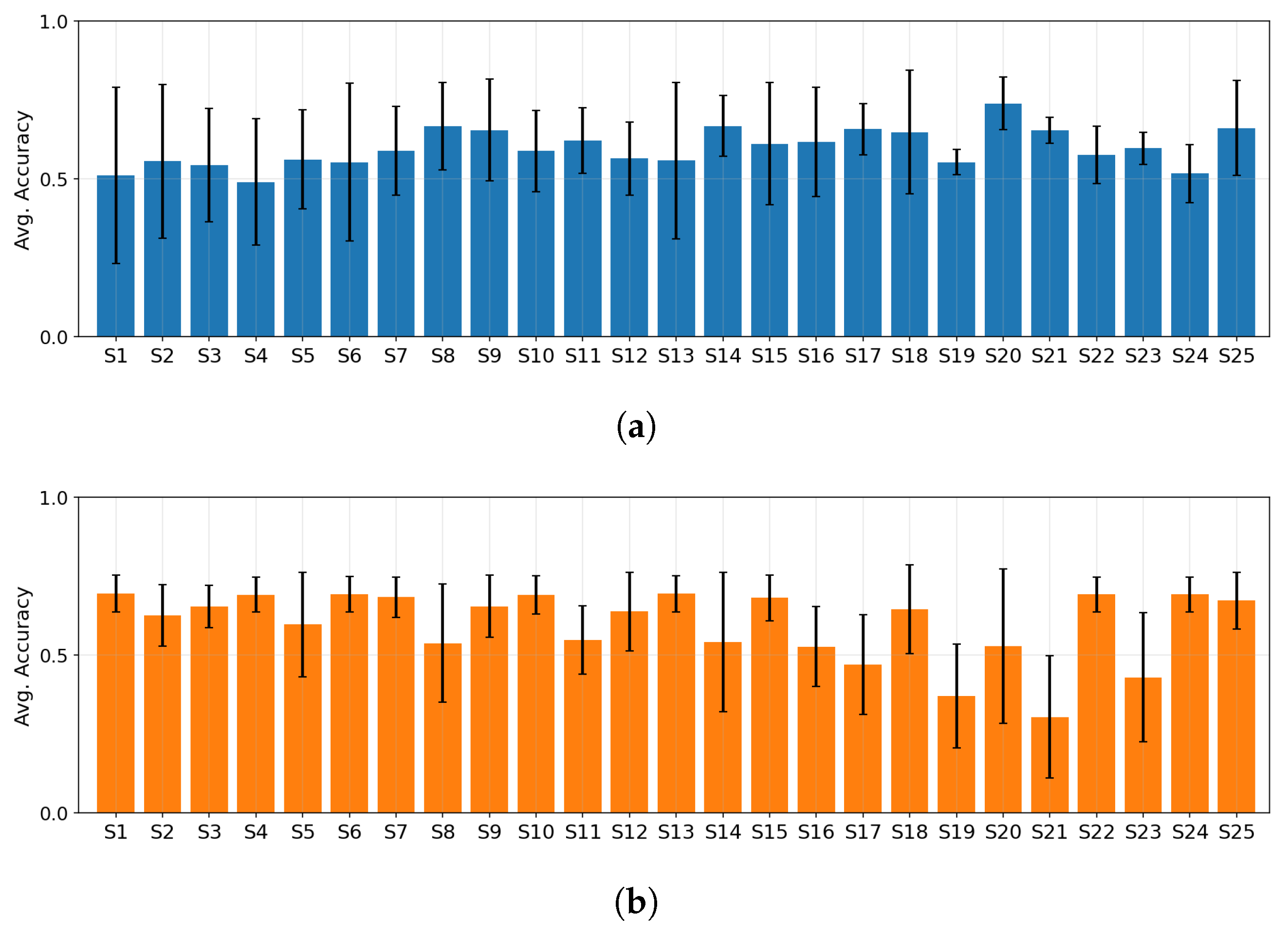
4.1. Individual Subject Model

The performance of each CNN model trained on data from each of the 25 individual subjects is shown in Figure 4. In addition to the random chance level performance (accuracy of 1/3), the performance of a naive model that builds a prediction based on the majority class is shown using empty bars. A naive model produces a constant output as it always predicts the class that has the highest prior probability. Since the time duration taken by each subject for writing and resting activity varies, the number of feature vectors extracted from each segments also varies, producing different prior probabilities. In this experiment, writing segments are longer than listening and resting for all subjects; thus, the writing class constitutes the majority class and a naive model always predicts the writing class for each input.

The test performance of every CNN model was found to be better than random chance. Compared to the naive model, the proposed CNN architecture performs well for all subjects except for subjects 16 and 17. It is interesting to observe that the same CNN architecture trained on different individuals performs differently. By optimizing the CNN architecture for individual subjects, the performance could have been improved. However, for comparative purposes, CNN models always followed the same architecture shown in Figure 3.

Figure 5 shows the Receiver Operating Characteristics (ROC) curves plot for all the models, which results in an average Area Under the Curve (AUC) of 0.86. This indicates that on average, models were performing well.

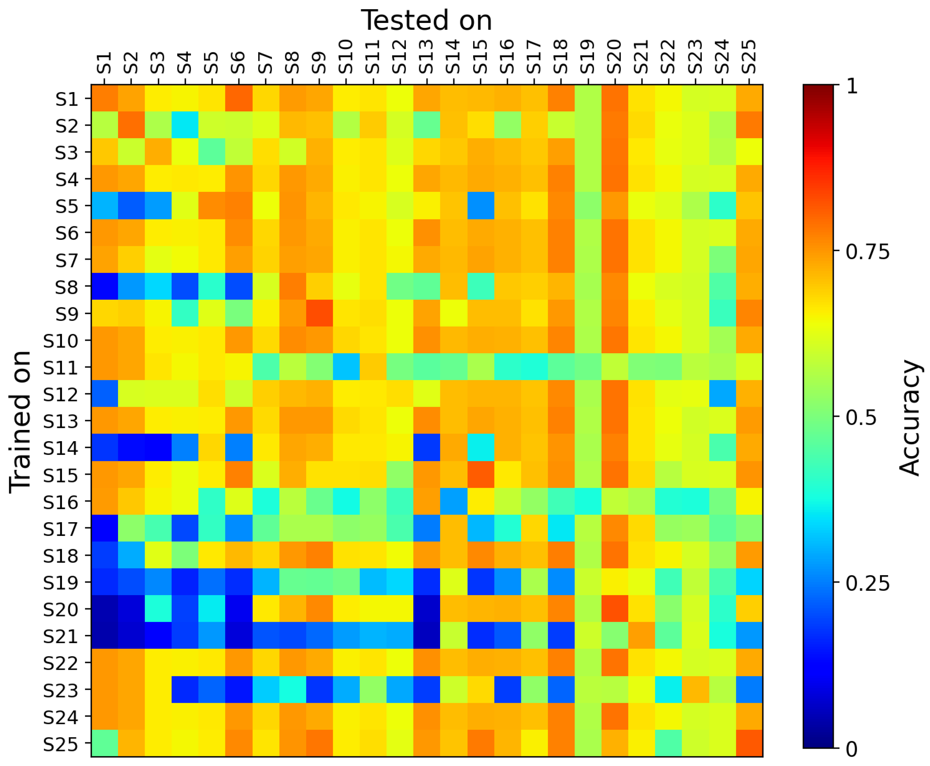
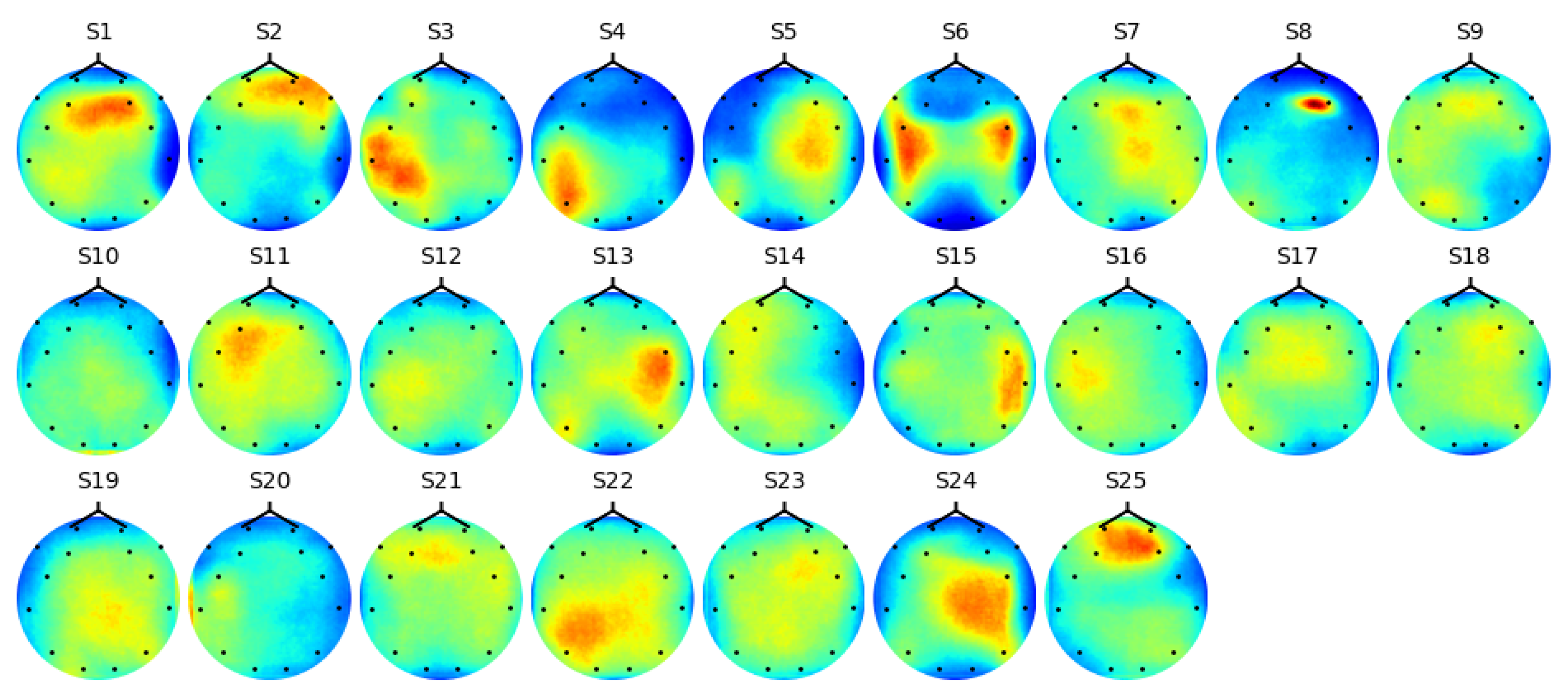
4.2. Inter-Subject Dependency Analysis

The results of the ISD analysis are shown in Figure 6 and Figure 7. Figure 6 shows a matrix representing the performance of the CNN models trained on each subject and tested on all 25 subjects. It is interesting to note that this matrix is not symmetric. Symmetry would have suggested that the performance of a model trained on subject A and tested on subject B is similar to the performance of a model trained on subject B and tested on subject A. It can be observed that compared to other models, the CNN model trained on subject S1 performs well on the other subjects. In contrast, the CNN model trained on subject S19 and S21 performs poorly on the other subjects. The results from Figure 6 can be summarized in two other plots, namely the average performance of all the trained models when tested on data from one single subject, as shown in Figure 7a, and the average performance of each model when tested on data from other subjects, as shown in Figure 7b. Figure 7b highlights that the model trained on S1 performs well on data from the other subjects, with a very low variability in performance. In contrast, Figure 7a indicates that the average performance of the models trained on every subject but S1 is low, with high variability when tested on data from S1. The performance of all the models tested on S19 and S21 is consistently higher than 0.5.

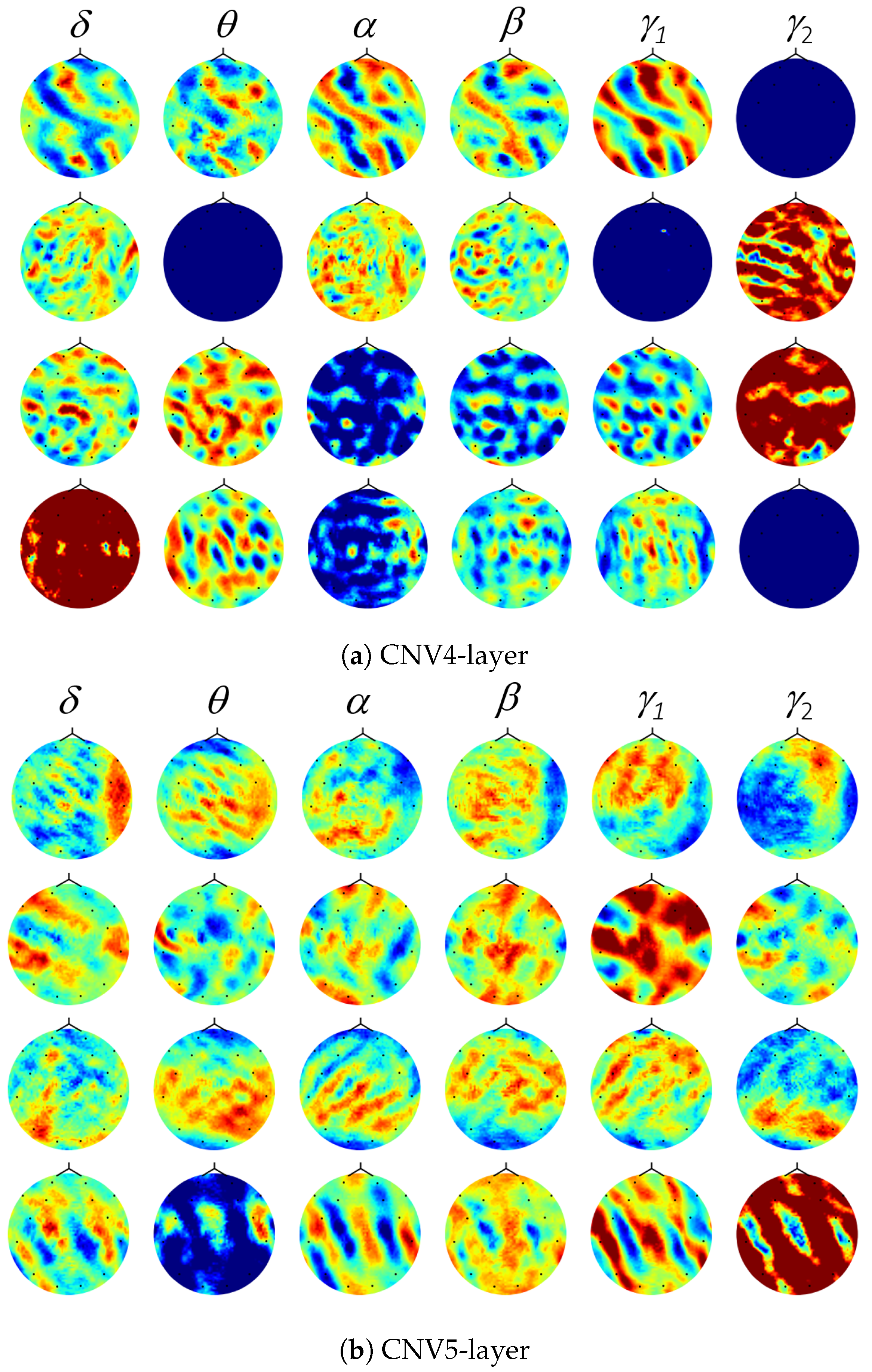
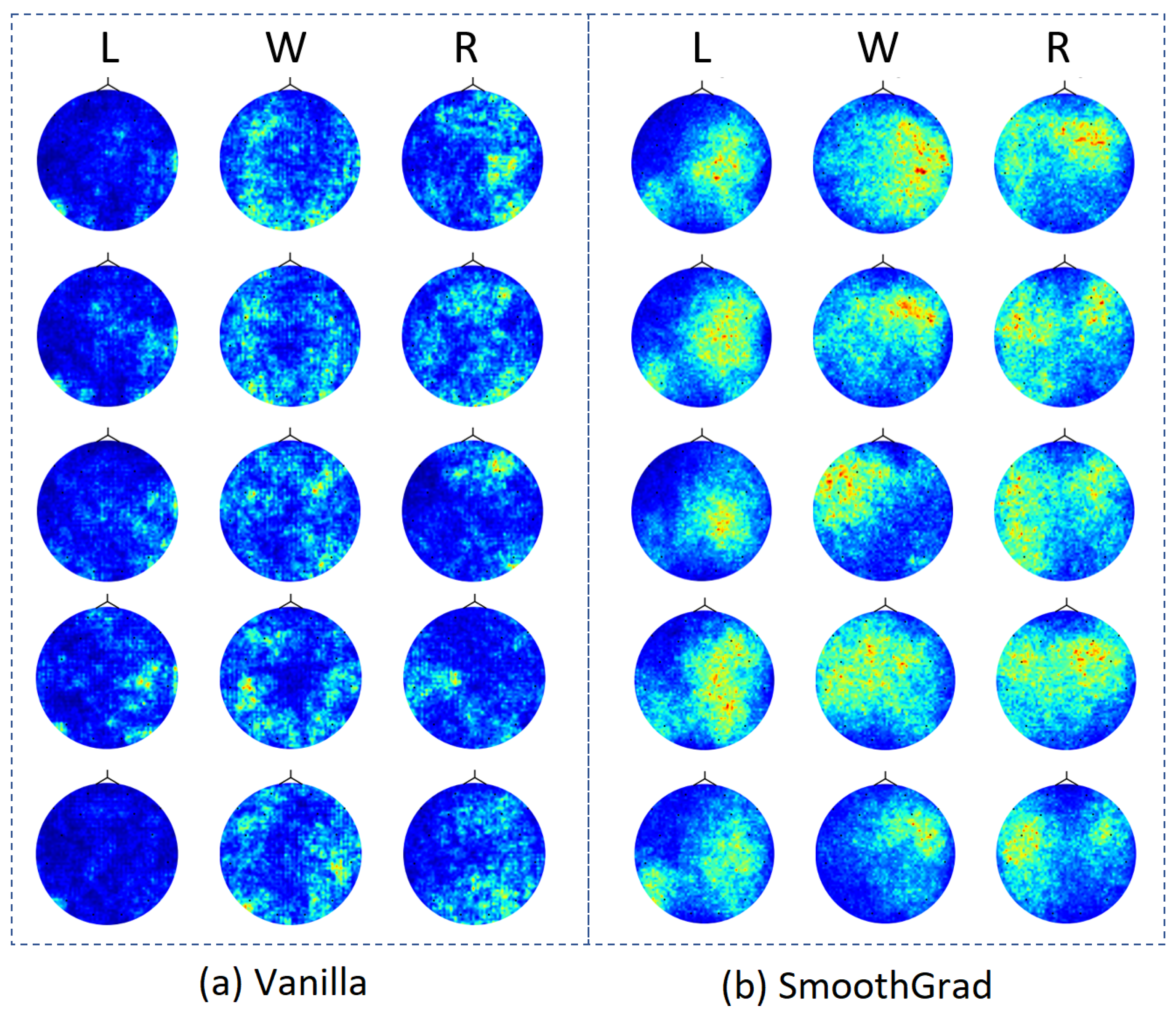
4.3. Deep Representation

A selection of four typical SSFI patterns associated with deep representations in each of the CNV layers in one of the trained CNN models is shown in Figure 8 and Figure 9. To facilitate their interpretation, each generated pattern is displayed as six separate topographical images corresponding to each of the frequency bands that define our SSFI structure.

It is interesting to observe that the SSFI patterns associated with layer CNV1 are focused on large brain regions in different frequency bands. For example, the first topographic map in the theta ($\theta$) frequency band (first row, second column) shown in Figure 8a reveals a comparison between two halves of the brain. More specifically, if the two halves of the brain exhibit opposite activities in the ($\theta$) frequency band, this particular pattern is activated, i.e., the respective neuron in the CVN1 layer is activated). As described in [42], the orientation of a pattern should not be interpreted as fixed. Therefore, the second map of the first pattern in Figure 8a should be interpreted as a comparison between any two halves of the brain. Specifically, if any two halves of the brain exhibit opposite activities in the ($\theta$) frequency band, this particular neuron in CNV1 will be activated. Similar patterns are seen across filters corresponding to different frequency bands. In general, the patterns from layer CNV1, also known as low-level features, compare the brain activity between large regions of the brain. The existing literature that analyzes deep representations, such as [42], suggests that the generated patterns can have any orientation. This statement would apply to conventional scenarios, such as those including images of natural objects. However, SSFIs have a fixed orientation corresponding to a constant topography; hence, this allows us to interpret SSFI patterns exactly as they are revealed and exclude changes in orientation. For instance, an SSFI pattern highlighting the left and right halves of the brain should not be interpreted as any two halves of the brain. The top first map in the alpha ($\alpha$) frequency band shown in Figure 8a (first row, third column) reveals that the associated neuron focuses on the temporal lobe activity, more on the left temporal lobe than the right. Another example worth observing is the third pattern of the delta ($\delta$) frequency band (third row, first column). This pattern reveals that the associated neuron is focusing on the high activity of the frontal side of brain (FC5, F3, AF4, F4, and F8) and the low activity of the parietal side of brain (P7, O1, T8). In general, similar patterns are seen across filters corresponding to different frequency bands. In summary, these patterns demonstrate that layer CNV1 produces low-level features that compare the brain activity between large regions of the brain. In contrast, low-level features produced by conventional CNN models for problems involving data structures such as images of the natural world correspond to edges and textures.

Compared to the SSFI patterns from layer CNV1, in layers CNV2 and CNV3, patterns are typically focused on very small regions. Layers CVN2 and CNV3 also present SSFIs that have dead channels. A dead channel is one which produces zero or constant response. Examples of dead channels are the ones producing the second, third, and sixth maps in the first pattern (first row) of Figure 8b. In an SSFI pattern, dead channels are useful for producing features that depend on a subset of frequency bands, while the others are excluded. For example, the first pattern in Figure 8b shows that the corresponding filter in layer CNV2 produces an output that uses information from the $\delta$, $\beta$, and ${\gamma }_1$ frequency bands only.

This suggests that layers CNV2 and CNV3 produce features that focus on different frequency bands. Interestingly, the number of dead channels decreases for layer CNV4 and there are almost none in layer CNV5, as shown in Figure 9. This indicates that CNV4 and CNV5 layers do combine features from all the channels in the previous layers, i.e., no channel is being filtered out. From Figure 9, it can be concluded that layers CNV4 and CNV5, which produce high-level features, focus on more localized areas of the brain. This contrasts with the low-level features produced by CNV1, which focus on larger regions.

To identify the association of brain regions and auditory task in the PhyAAt dataset, we further computed SSFI saliency maps using the Vanilla and SmoothGrad approaches. We extracted the top five SSFI arrays of subject S5 that were correctly classified by the CNN model trained on S5 and produced the saliency maps for each task (listening, writing, and resting). Saliency maps are shown in Figure 10. Unlike the conventional approach of displaying saliency maps over input images, Figure 10 displays SSFI saliency maps alone to highlight the relevant regions of the brain. This is a suitable visualization in our scenario, since the topography remains constant. Figure 10 reveals that the CNN model under investigation is looking into roughly the same region of the brain in each task, i.e., listening, writing, and resting, with slight variations. SmoothGrad saliency maps suggest that during a listening task, the CNN model focuses more on the right side of the brain.

To identify the common brain regions where each CNN model focuses to produce a correct prediction, we averaged SSFI saliency maps corresponding the top the 100 SSFI input arrays. A similar approach was used in [43] to localize the importance of an ECG signal in a DNN study. The averaged saliency maps during listening tasks for all the 25 subjects are shown in Figure 11, and allow us to identify the region of the brain that each CNN model is attending to during a listening task. Average saliency maps indicate that the brain regions associated with listening tasks are different in each subject, which might explain why models trained on one subject might perform poorly on other subjects [4]. Identifying subjects such that CNN models trained on them use common brain regions could be useful. Interestingly S1, S2, and S25 exhibit the same region of brain activity, and so do S3 and S4. A detailed analysis of these patterns could potentially reveal the reason why a CNN model trained on one subject performs differently on different subjects. This approach could also allow us to explore the association of brain regions with different brain activities.

5. Conclusions and Discussion

Modern DNNs have become a popular approach in EEG studies [18,19,20,21]. From a computational point of view, trained DNNs are pipelines that produce multiple representations of their input, which are known as deep representations. Each deep representation encapsulates a set of features describing the input. Representations close to the input of trained DNNs are associated with low-level features, whereas deeper representations close to the output correspond to high-level features and can identify complex patterns in the DNN input.

Despite the promising results shown by DNN approaches in EEG studies, our understanding of the computational pipelines that they implement remains limited. Understanding DNN pipelines and the deep representations that they produce can be useful. First, this would allow us to identify which EEG patterns are relevant for a specific prediction, which could shed light on the brain mechanisms involved. Second, by comparing deep representations from DNNs trained on EEG from different individuals, we can identify similarities and differences that could suggest different brain mechanisms. This would in turn allow us to cluster individuals according to the brain mechanisms that they exhibit. Third, understanding DNN pipelines and deep representations could contribute to realizing effective transfer learning and reduce training time. Transfer learning approaches can be used to retrain an existing DNN so that it can be used on other individuals or can be applied to predictive tasks different from the one for which the DNN was originally trained.

In this article, we have presented an approach that allows us to interpret the deep representations of DNN models trained on EEG multi-channel data. The proposed approach exploits the spatio-spectral relationship of EEG data and generates SSFI patterns revealing the frequency bands and the spatial region of brain that activate the neurons within each layer in a DNN model. The association between brain regions and frequency bands and physical, physiological, and psychological activities is widely accepted in neuroscience, and hence, SSFI patterns provide us with meaningful interpretations of the deep representations produced by DNN models. SSFI patterns interpreting deep representations can therefore enhance our understanding of the brain activity. With BCI systems in mind, SSFI patterns can also contribute to the design and realization of transfer learning.

To evaluate our approach, we used the PhyAAt dataset for auditory tasks. We trained 25 CNN models on EEG multi-channel signals from each subject in the dataset. First, we analyzed the performance of each individual CNN model on EEG signals from the subject it was trained on. Then we conducted ISD analysis, which allowed us to investigate how a model trained on one subject performs on others. The observed variation in performance demonstrates the importance of learning robust deep representations, which are necessary to implement transfer learning effectively.

We analyzed the SSFI patterns associated with the deep representation generated by neurons in each of the layers of the trained CNN models. To generate SSFI patterns, we used an activation maximization approach. SSFI saliency maps for listening, writing, and resting tasks were also produced and averaged saliency maps were obtained to highlight the common brain regions that are associated with listening tasks for all the subjects. Our approach and subsequent analysis reveals that, unlike conventional CNN scenarios such as those involving images of the natural world, SSFI low-level features represent the activities in larger brain regions and high-level features represent clusters of small brain regions. Interestingly, middle-level features are used to selectively combine different frequency bands. The common brain regions extracted by averaged SSFI saliency maps show different regions associated with listening tasks for different subjects, and reveal that a few subjects share similar brain regions.

We have applied our approach to investigating deep representations to CNN models trained on multi-channel EEG signals recorded during auditory tasks. Our approach could also be applied to explore deep representations in DNN models trained on EEG signals recorded during other brain tasks, for instance, visual tasks. The same methodology that we have implemented in this study could be followed to analyze similarities and differences between the brain activity in different individuals carrying out the same brain task.

References

1. Wolpaw, J.R.; Birbaumer, N.; McFarland, D.J.; Pfurtscheller, G.; Vaughan, T.M. Brain–Computer interfaces for communication and control. Clin. Neurophysiol. 2002, 113, 767–791. [Google Scholar] [CrossRef] [PubMed]
2. Bellotti, F.; Kapralos, B.; Lee, K.; Moreno-Ger, P.; Berta, R. Assessment in and of serious games: An overview. Adv. Hum. Comput. Interact. 2013, 2013, 136864. [Google Scholar] [CrossRef]
3. Paranthaman, P.K.; Bajaj, N.; Solovey, N.; Jennings, D. Comparative evaluation of the EEG performance metrics and player ratings on the virtual reality games. In Proceedings of the 2021 IEEE Conference on Games (CoG), Copenhagen, Denmark, 17–20 August 2021; IEEE: Piscataway, NJ, USA, 2021; pp. 1–8. [Google Scholar]
4. Lazar, N.A.; Luna, B.; Sweeney, J.A.; Eddy, W.F. Combining brains: A survey of methods for statistical pooling of information. Neuroimage 2002, 16, 538–550. [Google Scholar] [CrossRef]
5. Tu, W.; Sun, S. A subject transfer framework for EEG classification. Neurocomputing 2012, 82, 109–116. [Google Scholar] [CrossRef]
6. Sun, S.; Zhou, J. A review of adaptive feature extraction and classification methods for EEG-based brain-computer interfaces. In Proceedings of the 2014 International Joint Conference on Neural Networks (IJCNN), Vancouver, BC, Canada, 24–29 July 2016; IEEE: Piscataway, NJ, USA, 2014; pp. 1746–1753. [Google Scholar]
7. Zhang, Y.Q.; Zheng, W.L.; Lu, B.L. Transfer components between subjects for EEG-based driving fatigue detection. In Proceedings of the International Conference on Neural Information Processing, Istanbul, Turkey, 9–12 November 2015; Springer: Berlin/Heidelberg, Germany, 2015; pp. 61–68. [Google Scholar]
8. Kang, H.; Nam, Y.; Choi, S. Composite common spatial pattern for subject-to-subject transfer. IEEE Signal Process. Lett. 2009, 16, 683–686. [Google Scholar] [CrossRef]
9. Devlaminck, D.; Wyns, B.; Grosse-Wentrup, M.; Otte, G.; Santens, P. Multisubject learning for common spatial patterns in motor-imagery BCI. Comput. Intell. Neurosci. 2011, 2011, 8. [Google Scholar] [CrossRef] [PubMed]
10. Samek, W.; Meinecke, F.C.; Müller, K.R. Transferring subspaces between subjects in brain–computer interfacing. IEEE Trans. Biomed. Eng. 2013, 60, 2289–2298. [Google Scholar] [CrossRef] [PubMed]
11. Lotte, F.; Guan, C. Learning from other subjects helps reducing brain-computer interface calibration time. In Proceedings of the 2010 IEEE International Conference on Acoustics, Speech and Signal Processing, Dallas, TX, USA, 14–19 March 2010; IEEE: Piscataway, NJ, USA, 2010; pp. 614–617. [Google Scholar]
12. Yuan, P.; Chen, X.; Wang, Y.; Gao, X.; Gao, S. Enhancing performances of SSVEP-based brain–computer interfaces via exploiting inter-subject information. J. Neural Eng. 2015, 12, 046006. [Google Scholar] [CrossRef]
13. Völker, M.; Schirrmeister, R.T.; Fiederer, L.D.; Burgard, W.; Ball, T. Deep transfer learning for error decoding from non-invasive EEG. In Proceedings of the 2018 6th International Conference on Brain-Computer Interface (BCI), Gangwon, Republic of Korea, 15–17 January 2018; IEEE: Piscataway, NJ, USA, 2018; pp. 1–6. [Google Scholar]
14. Dalhoumi, S.; Dray, G.; Montmain, J. Knowledge transfer for reducing calibration time in brain-computer interfacing. In Proceedings of the 2014 IEEE 26th International Conference on Tools with Artificial Intelligence, Limassol, Cyprus, 10–12 November 2014; IEEE: Piscataway, NJ, USA, 2014; pp. 634–639. [Google Scholar]
15. Wan, Z.; Yang, R.; Huang, M.; Zeng, N.; Liu, X. A review on transfer learning in EEG signal analysis. Neurocomputing 2021, 421, 1–14. [Google Scholar] [CrossRef]
16. Sanei, S.; Chambers, J.A. EEG Signal Processing; John Wiley & Sons: Hoboken, NJ, USA, 2013. [Google Scholar]
17. Lemm, S.; Blankertz, B.; Curio, G.; Muller, K.R. Spatio-spectral filters for improving the classification of single trial EEG. IEEE Trans. Biomed. Eng. 2005, 52, 1541–1548. [Google Scholar] [CrossRef]
18. Roy, Y.; Banville, H.; Albuquerque, I.; Gramfort, A.; Falk, T.H.; Faubert, J. Deep learning-based electroencephalography analysis: A systematic review. J. Neural Eng. 2019, 16, 051001. [Google Scholar] [CrossRef] [PubMed]
19. Altaheri, H.; Muhammad, G.; Alsulaiman, M.; Amin, S.U.; Altuwaijri, G.A.; Abdul, W.; Bencherif, M.A.; Faisal, M. Deep learning techniques for classification of electroencephalogram (EEG) motor imagery (MI) signals: A review. Neural Comput. Appl. 2023, 35, 14681–14722. [Google Scholar] [CrossRef]
20. Al-Saegh, A.; Dawwd, S.A.; Abdul-Jabbar, J.M. Deep learning for motor imagery EEG-based classification: A review. Biomed. Signal Process. Control. 2021, 63, 102172. [Google Scholar] [CrossRef]
21. Craik, A.; He, Y.; Contreras-Vidal, J.L. Deep learning for electroencephalogram (EEG) classification tasks: A review. J. Neural Eng. 2019, 16, 031001. [Google Scholar] [CrossRef]
22. Zhang, D.; Yao, L.; Zhang, X.; Wang, S.; Chen, W.; Boots, R. EEG-based intention recognition from spatio-temporal representations via cascade and parallel convolutional recurrent neural networks. arXiv 2017, arXiv:1708.06578. [Google Scholar]
23. Nurse, E.S.; Karoly, P.J.; Grayden, D.B.; Freestone, D.R. A generalizable brain-computer interface (BCI) using machine learning for feature discovery. PLoS ONE 2015, 10, e0131328. [Google Scholar] [CrossRef]
24. Nurse, E.; Mashford, B.S.; Yepes, A.J.; Kiral-Kornek, I.; Harrer, S.; Freestone, D.R. Decoding EEG and LFP signals using deep learning: Heading TrueNorth. In Proceedings of the ACM International Conference on Computing Frontiers, New York, NY, USA, 16–19 May 2016; ACM: New York, NY, USA, 2016; pp. 259–266. [Google Scholar]
25. Stober, S.; Sternin, A.; Owen, A.M.; Grahn, J.A. Deep feature learning for EEG recordings. arXiv 2015, arXiv:1511.04306. [Google Scholar]
26. Bashivan, P.; Rish, I.; Yeasin, M.; Codella, N. Learning representations from EEG with deep recurrent-convolutional neural networks. arXiv 2015, arXiv:1511.06448. [Google Scholar]
27. Chambon, S.; Galtier, M.N.; Arnal, P.J.; Wainrib, G.; Gramfort, A. A deep learning architecture for temporal sleep stage classification using multivariate and multimodal time series. IEEE Trans. Neural Syst. Rehabil. Eng. 2018, 26, 758–769. [Google Scholar] [CrossRef] [PubMed]
28. Sors, A.; Bonnet, S.; Mirek, S.; Vercueil, L.; Payen, J.F. A convolutional neural network for sleep stage scoring from raw single-channel EEG. Biomed. Signal Process. Control. 2018, 42, 107–114. [Google Scholar] [CrossRef]
29. Tjepkema-Cloostermans, M.C.; de Carvalho, R.C.; van Putten, M.J. Deep learning for detection of focal epileptiform discharges from scalp EEG recordings. Clin. Neurophysiol. 2018, 129, 2191–2196. [Google Scholar] [CrossRef]
30. Thodoroff, P.; Pineau, J.; Lim, A. Learning robust features using deep learning for automatic seizure detection. In Proceedings of the Machine Learning for Healthcare Conference, Los Angeles, CA, USA, 19–20 August 2016; PMLR: New York, NY, USA, 2016; pp. 178–190. [Google Scholar]
31. Ruffini, G.; Ibañez, D.; Castellano, M.; Dubreuil-Vall, L.; Soria-Frisch, A.; Postuma, R.; Gagnon, J.F.; Montplaisir, J. Deep learning with EEG spectrograms in rapid eye movement behavior disorder. Front. Neurol. 2019, 10, 806. [Google Scholar] [CrossRef]
32. Zhao, H.; Zheng, Q.; Ma, K.; Li, H.; Zheng, Y. Deep representation-based domain adaptation for nonstationary EEG classification. IEEE Trans. Neural Netw. Learn. Syst. 2020, 32, 535–545. [Google Scholar] [CrossRef] [PubMed]
33. Tan, C.; Sun, F.; Zhang, W. Deep transfer learning for EEG-based brain computer interface. In Proceedings of the 2018 IEEE International Conference on Acoustics, Speech and Signal Srocessing (ICASSP), Calgary, AB, Canada, 15–20 April 2018; IEEE: Piscataway, NJ, USA, 2018; pp. 916–920. [Google Scholar]
34. Bajaj, N.; Requena-Carrión, J.; Bellotti, F. PhyAAt: Physiology of Auditory Attention to Speech Dataset. arXiv 2020, arXiv:arXiv:2005.11577. [Google Scholar]
35. Choi, M.; Jeong, J.J. Comparison of Selection Criteria for Model Selection of Support Vector Machine on Physiological Data with Inter-Subject Variance. Appl. Sci. 2022, 12, 1749. [Google Scholar] [CrossRef]
36. Lee, P.; Hwang, S.; Lee, J.; Shin, M.; Jeon, S.; Byun, H. Inter-subject contrastive learning for subject adaptive eeg-based visual recognition. In Proceedings of the 2022 10th International Winter Conference on Brain-Computer Interface (BCI), Gangwon-do, Republic of Korea, 21–23 February 2022; IEEE: Piscataway, NJ, USA, 2022; pp. 1–6. [Google Scholar]
37. Gramfort, A.; Luessi, M.; Larson, E.; Engemann, D.A.; Strohmeier, D.; Brodbeck, C.; Parkkonen, L.; Hämäläinen, M.S. MNE software for processing MEG and EEG data. Neuroimage 2014, 86, 446–460. [Google Scholar] [CrossRef]
38. Bajaj, N.; Carrión, J.R.; Bellotti, F.; Berta, R.; De Gloria, A. Automatic and tunable algorithm for EEG artifact removal using wavelet decomposition with applications in predictive modeling during auditory tasks. Biomed. Signal Process. Control. 2020, 55, 101624. [Google Scholar] [CrossRef]
39. Krizhevsky, A.; Sutskever, I.; Hinton, G.E. Imagenet classification with deep convolutional neural networks. In Proceedings of the Advances in Neural Information Processing Systems, Lake Tahoe, NV, USA, 3–6 December 2012; pp. 1097–1105. [Google Scholar]
40. Zeiler, M.D.; Fergus, R. Visualizing and understanding convolutional networks. In Proceedings of the European Conference on Computer Vision, Munich, Germany, 8–14 September 2014; Springer: Berlin/Heidelberg, Germany, 2014; pp. 818–833. [Google Scholar]
41. Simonyan, K.; Vedaldi, A.; Zisserman, A. Deep inside convolutional networks: Visualising image classification models and saliency maps. arXiv 2013, arXiv:1312.6034. [Google Scholar]
42. Erhan, D.; Bengio, Y.; Courville, A.C.; Vincent, P. Visualizing Higher-Layer Features of a Deep Network; University of Montreal: Montreal, QC, Canada, 2009. [Google Scholar]
43. Sau, A.; Giatti, L.; Ng, F.S.; Peters, N.; Shipley, M.; Barreto, S.; Pastika, L.; Ribeiro, A.; Sabino, E.; Ware, J.; et al. 88 Exploring the prognostic significance and important phenotypic and genotypic associations of neural network-derived electrocardiographic features. Heart 2023, 109, A96–A99. [Google Scholar] [CrossRef]
Figure 1. Prediction pipeline consisting of an SSFI processing stage followed by a CNN model. Small windows t 1 , t 2 , …, t N are extracted from a 14-channel EEG, transformed into SSFI, and then fed into the CNN model.
Applsci 13 09825 g001
Figure 2. Spatial power distribution for a single frequency band on a topographic map and its corresponding SSFI on a rectangular grid. The spatial power distribution is obtained from a 14-channel EEG segment whose recording electrodes are identified on the topography.
Applsci 13 09825 g002
Figure 3. CNN architecture used for the ternary listening–writing–reading classification task. It consists of five convolution layers followed by two fully connected layers.
Applsci 13 09825 g003
Figure 4. Performance of each CNN model trained and tested on the same individual subject. Empty bars represent the performance of the majority-based model and the black horizontal line represents the random chance-level performance, i.e., 1/3.
Applsci 13 09825 g004
Figure 5. ROC curve of all the 25 CNN models relating true positive rate (TPR) and false positive rate (FPR) values.
Applsci 13 09825 g005
Figure 6. Inter-subject dependency analysis matrix that represents the performance of each CNN model on every subject.
Applsci 13 09825 g006
Figure 7. (a) Average performance of every trained CNN model when tested on one single subject, where the horizontal axis represents the test subject. (b) Average performance of each CNN model when tested on all the subjects, where the horizontal axis represents the training subject.
Applsci 13 09825 g007
Figure 8. Selection of typical SSFI deep representation patterns corresponding to four filters at layers (a) CNV1, (b) CNV2, and (c) CNV3 for subject S5. Each pattern is shown as a row, and consists of six maps corresponding to each frequency band arranged in columns.
Applsci 13 09825 g008
Figure 9. Selection of typical SSFI deep representation patterns corresponding to four filters at layers (a) CNV4 and (b) CNV5 for subject S5. Patterns are shown as rows, frequency bands as columns.
Applsci 13 09825 g009
Figure 10. Saliency maps for top five SSFI input arrays for listening (L), writing (W), and resting (R) tasks that were classified correctly. Saliency maps are generated using (a) Vanilla (b) SmoothGrad approach.
Applsci 13 09825 g010
Figure 11. Average saliency map of listening task for all 25 subjects.
Applsci 13 09825 g011
Disclaimer/Publisher’s Note: The statements, opinions and data contained in all publications are solely those of the individual author(s) and contributor(s) and not of MDPI and/or the editor(s). MDPI and/or the editor(s) disclaim responsibility for any injury to people or property resulting from any ideas, methods, instructions or products referred to in the content.