Speaker Recognition Based on Dung Beetle Optimized CNN

Abstract

Speaker recognition methods based on convolutional neural networks (CNN) have been widely used in the security field and smart wearable devices. However, the traditional CNN has many hyperparameters that are difficult to determine, making the model easily fall into local optimum or even fail to converge during the training process. Intelligent algorithms such as particle swarm optimization and genetic algorithms are used to solve the above problems. However, these algorithms perform poorly compared to the current emerging meta-heuristic algorithms. In this study, the dung beetle optimized convolution neural network (DBO-CNN) is proposed to identify the speakers for the first time, which is helpful in finding suitable hyperparameters for training. By testing the dataset of 50 people, it was demonstrated that the accuracy of the model was significantly improved by using this approach. Compared with the traditional CNN and CNN optimized by other intelligent algorithms, the average accuracy of DBO-CNN has increased by 1.22~4.39% and reached 97.93%.

1. Introduction

As an inherent biological attribute of human beings, voiceprint can be used to assist in identity verification. Speaker recognition developed from voiceprint has become an indispensable technology in the financial industry and private devices. Thullier et al. applied speaker recognition technology to mobile devices [1]. The main voiceprint feature extraction methods include the Linear Prediction Coding [2], the Linear Prediction Cepstral Coefficients (LPCC) [3,4], and the Mel-Frequency Cepstral Coefficients (MFCC) [5,6]. Based on the above methods, a large number of mature recognition models and applications have been proposed. Nakagawa et al. proposed a text-independent speaker recognition method based on the Hidden Markov models (HMM) and the Gaussian mixture model (GMM). They evaluated the robustness of the model affected by speech style [7]. Matsui et al. proposed a method to combine the speaker and the noise source into a noisy speaker HMM with a specific signal-to-noise ratio (SNR) and use this likelihood value to obtain the recognition result [8]. Limkar et al. proposed to compare the recognition rates of multiple combination models using vector quantization and dynamic time warping, and the results showed that LPCC and MFCC had better performance [9]. Zheng et al. proposed the GMM Universal Background Model, which utilized the speaker’s trained speech and a Bayesian adaptive form to adjust the parameters of UBM [10]. The structural constraint is a major drawback of the above models, which may not be sufficient to model tasks when faced with complex tasks [11].

Non-parametric models have better flexibility and performance. Keogh et al. introduced a new technology for precise indexing, which was a model based on template matching, which solved the problem of different pronunciation lengths, but it could only be used in isolated word speech recognition [12]. Campbell et al. proposed the use of GMM supervectors in a support vector machine (SVM) classifier and produced excellent classification accuracy in speaker recognition [13]. However, the performance of the above models is highly susceptible to environmental noise, often resulting in a sharp drop in recognition rate.

CNN has been widely used in the fields of image classification and object detection due to its excellent feature extraction ability. In speaker recognition, CNN achieved good results in classifying spectrograms, with significantly improved anti-noise performance [14,15]. Achar et al. proposed a hybrid recognition method based on CNN and MFCC, which achieved a recognition accuracy of 87.5% [16]. Liu et al. proposed a new model to improve the recognition accuracy of short speech speaker recognition systems by addressing the issue of GMM being unable to recognize short speech speakers accurately and reducing the recognition error rate from 4.9% to 2.5% [17]. Joonet et al. created the VoxCeleb2 dataset and used a deep CNN to classify it with 92.67% accuracy [18]. Jagiasi et al. described a text-independent CNN model for speaker recognition and achieved recognition rates from 75% to 85% [19]. Wang et al. proposed a voiceprint recognition model based on Mel time-spectrum convolutional neural network for identifying faults in transformers during operation. This method constructed a CNN model by feature extraction preprocessing and Mel filter. This model could recognize the voiceprint of transformers by four different operating faults [20]. However, the hyperparameters of these models are mostly manually tuned, which requires experience and skill; thus, obtaining the highest-performing CNN models is time-consuming [21]. Sometimes, the hyperparameters set based on experience will make the model fall into a local optimal solution or even fail to converge.

Recently, many scholars have devoted themselves to efficient optimization algorithms to tune the hyperparameters of CNNs. Swarm-based intelligent algorithms such as genetic algorithm (GA) and particle swarm optimization (PSO) were used to optimize the hyperparameters of CNN [22,23,24,25]. Yoo et al. proposed a method of optimizing CNN with GA and tested image recognition on the MNIST dataset and achieved an accuracy rate of 99.4% [22]. Ishaq et al. used GA to adjust the hyperparameters of CNN and achieved an accuracy rate of 95.5% in the emotion recognition test, which had a great advantage over other methods [23]. Chen et al. proposed a PSO-optimized adaptive CNN(PSO-CNN) to analyze the spectrogram during the working process of the bearing to determine whether the bearing was damaged. This method had a recognition accuracy rate of 99.9% for the four damage situations [24]. Bhuvansehwari et al. used the dragonfly optimizer based on information gain and the CNN classifier optimized by particle PSO based on depth clustering to identify network attack aircraft types. The optimization algorithm could reduce clustering losses and network losses [25]. The above studies showed that swarm-based optimization methods were effective in improving the performance of CNN. However, after decades of technological development, the above intelligent algorithms have shown limited effectiveness in current complex and huge engineering problems.

Researchers have proposed many heuristic search algorithms inspired by nature that imitate various biological habits. These bionics-based strategies have the outstanding features of high optimization power, high fast convergence, and excellent robustness and can be applied to optimize the hyperparameters of the network. The bionics-based algorithm has two core strategies for biological populations: role division and behavioral differentiation. Role division refers to the use of fitness to divide the population into different groups, while behavioral difference means that individuals in different groups have different action strategies. In population, the role played by each individual is not static. During the foraging process, the fitness of individuals will change, which will change their role. However, no matter how the population is divided, the ultimate goal of all individuals is the same, that is, to find the most suitable habitat for the survival and reproduction of the population. In particular, the action strategies of individuals in bionic algorithms are more reasonable and effective because the objects they imitate are multiplying and thriving in real life. In recent years, the Whale Algorithm [26], Grey Wolf Optimization [27], Sparrow Search Algorithm (SSA) [28], and Jumping Spider Optimization Algorithm [29] were heuristic algorithms proposed based on the above ideas, which were efficient search capabilities. They have been applied in many fields [30,31,32,33].

Based on the above analysis, the DBO is proposed to optimize the hyperparameters of CNN to improve the correct rate of speaker recognition and its anti-noise ability. DBO is the latest heuristic algorithm proposed by Xue et al., with excellent exploration and high local optimal avoidance ability [34]. In this algorithm, the stratum distribution and foraging habits in the dung beetle group are simulated, and the different foraging strategies to find the optimal solution within a certain range are used. In addition, a comparison between the DBO and the other algorithms is implemented, and the experimental results demonstrate the superiority of DBO in optimizing CNN hyperparameters. This is the first time DBO has been used for speaker recognition. The paper is structured as follows: Sec. II shows the processing flow of audio data. Sec. III introduces the CNN model architecture and DBO calculation process. Sec. IV shows the result and discussion about optimized CNN. Sec. V presents conclusions and future work.

2. Background

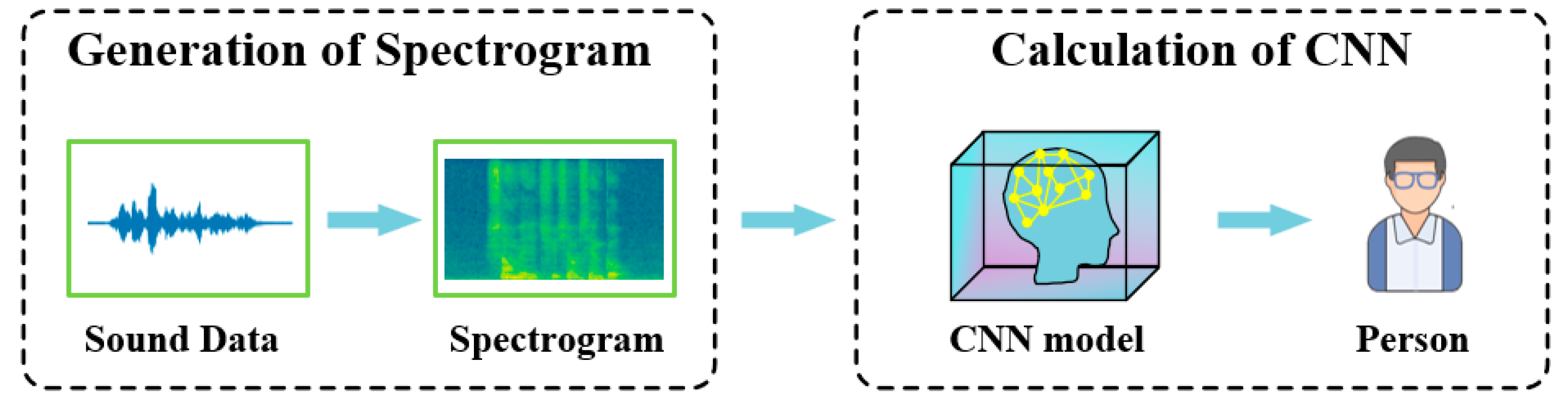
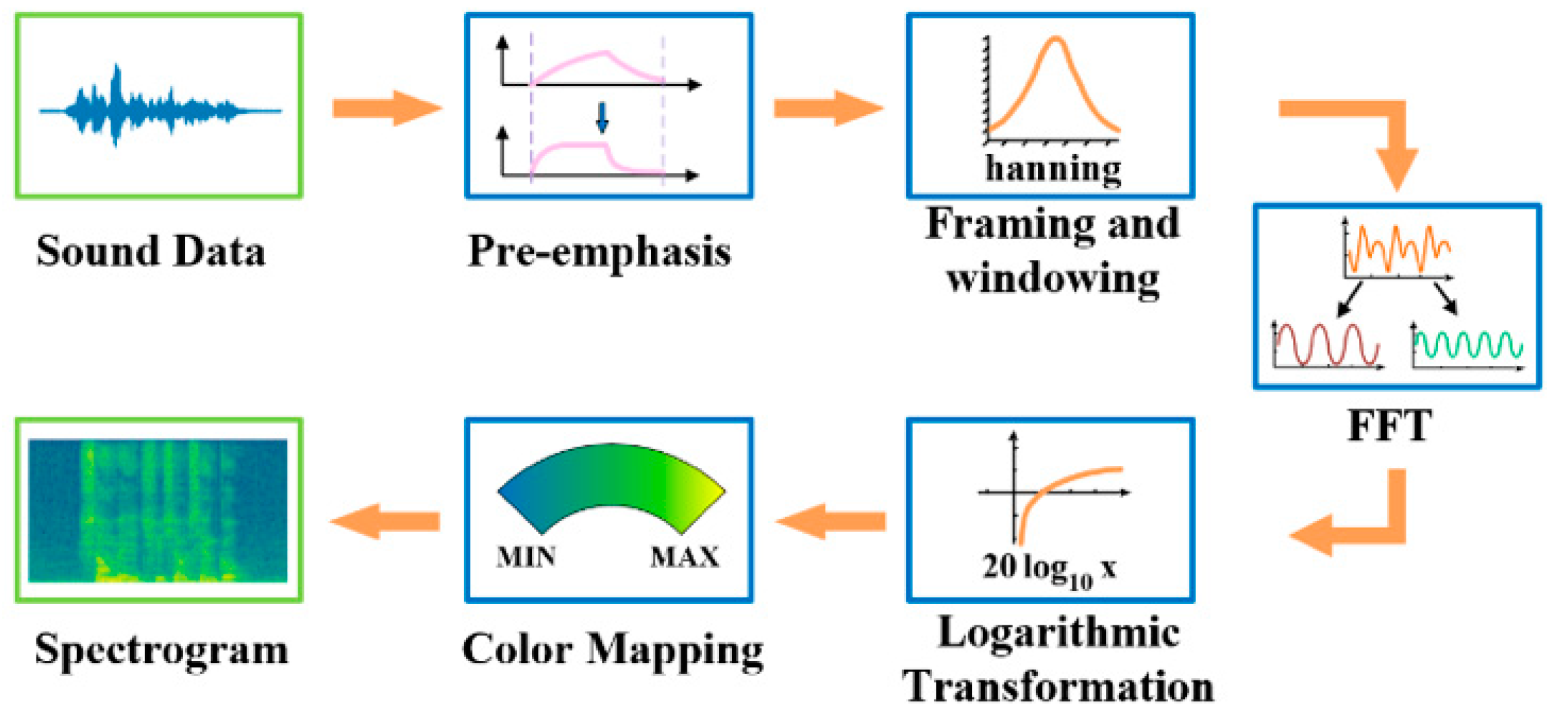
2.1. Generation of Spectrogram

The process of using CNN for speaker recognition includes two parts: the generation of the spectrogram and the calculation of CNN, as shown in Figure 1. Firstly, convert the audio signal into spectrum diagram data, and then import the obtained images into CNN for feature extraction and classification. Finally, accurately identify the speaker.

Since two-dimensional data is used in CNN, it is necessary to expand the dimension of audio data. The spectrogram is an image that displays the audio frequency spectrum, which denotes the variation of the frequency and amplitude of a speech signal over time. In the spectrogram, the energy of sound is displayed in the form of texture, which is called voiceprint. Voiceprint contains a lot of speaker characteristics, and everyone’s voiceprint is different. The essence of speaker recognition is to extract and classify voiceprints.

As shown in Figure 2, the production process of the spectrogram is divided into five steps: (i) pre-emphasis is used to enhance the high-frequency content of the signal to compensate for the loss during the acquisition process; (ii) due to the short-term stability of the voice signal, the audio signal is decomposed into some small fragments, and then the Hanning window is added to these fragments; (iii) the amplitude-frequency characteristics of the above speech segment sequence are obtained after the fast Fourier transform (FFT) processing, and then the modulus is taken to obtain the transformed linear spectrum; (iv) a linear spectrum is converted into a spectrogram by the logarithmic transformation; (v) color mapping is used to add details and features to the image and resize the image for CNN recognition.

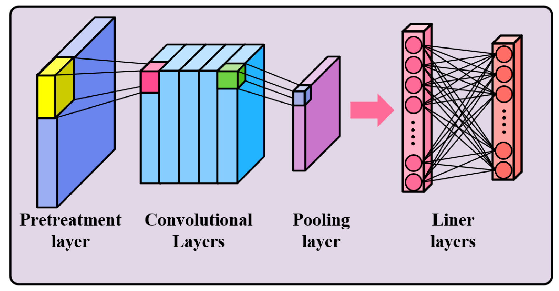
2.2. CNN Architecture

As shown in Figure 3, CNN can be functionally divided into two parts: feature extraction and classification. The feature extraction is composed of two-dimensional convolutional layers and pooling layers stacked in a certain order. The number of filters in each convolutional layer corresponds to the number of features currently expected to be extracted from the image, and the pooling layer abstracts it to a higher level while reducing the size of the image. The classification is the combination of the full connection layer and the activation function, which maps the extracted features to the sample space, and nonlinear calculations are utilized to improve the expressiveness of the network by the activation function.

When building a CNN, there are numerous hyperparameters that need to be determined. The hyperparameter types that this study focuses on are as follows:

• The number of filters per convolution layer; this parameter determines the abstraction ability of the network and the number of features to be eventually extracted
• The number of neurons in the fully connected layer; too few neurons may result in failure to train a model that meets the requirements, while numerous neurons may lead to overfitting
• Learning rate: If the learning rate is too low, it is easy for the model to fall into a local optimum, and if it is too high, it is easy to miss the global optimum and fail to complete the training.

Building and training CNN with good performance is not simple; it requires a lot of time and cost. Therefore, there is an urgent need for a method that can automatically build CNN in various tasks, which can help people determine various kinds of superparameters.

3. Materials and Methods

In this section, DBO is used to optimize the hyperparameters of CNN. A subset of the open-source voice dataset is employed. Section 3.1 introduces the dataset used in this article, Section 3.2 describes the CNN model, Section 3.3 describes the implementation principle of DBO, and Section 3.4 describes the detailed process of optimizing CNN by DBO.

3.1. Dataset

In order to verify the universality of the proposed method, two databases were used in this study. One is the Chinese Mandarin open-source speech database of AI-shell, which is produced by 400 people, covering areas such as voice control, autonomous driving, and industrial production. The other is VTCK, which is often used for average speech models trained on multiple speakers.

Fifty people were randomly selected from each of the two databases to construct the two datasets used in this study. These voices are cut into 2.5 s long segments, and each segment contains about 40,000 data points. When using FFT to make a spectrogram, set the length of the Hanning window to 256 and the moving width of each frame to 128, which is half of the window length. The obtained spectrograms are normalized to 128 × 128. The AI-shell data sets contain 17,265 images; the number of images is 14,605 for training sets and 3200 for test sets. The VTCK data sets contain images; the number of images is 14,226 for training sets and 3014 for test sets.

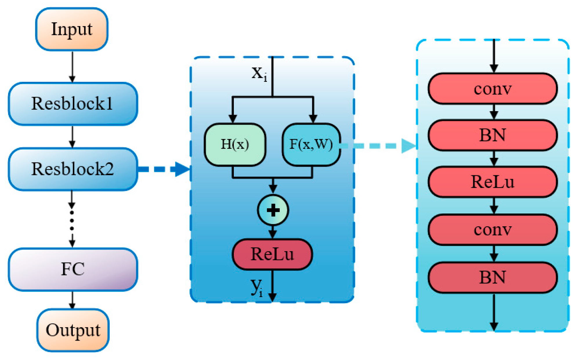
3.2. Residual Network (ResNet)

CNNs significantly outperform other traditional classifier models in the field of image recognition. However, as the depth of the model increases, problems such as gradient disappearance and gradient explosion will degrade the model and make the performance of the model worse. The fundamental reason is that the parameters of the deeper convolution kernel are difficult to be effectively adjusted in the later stage of training. ResNet is proposed to solve the above problems [35]. ResNet directly transmits low-level features to higher levels by introducing residual blocks, which makes it more capable of feature extraction and representation. This connection mode will not be affected by the depth of the network.

As shown in Figure 4, ResNet contains many residual blocks. There are two parts of each block: shortcut and convolution calculation. Shortcut maps the image of the previous layer directly to the next layer. The convolution calculation includes several convolution kernels, batch normalization (BN), and activation functions. BN aims to normalize the same batch of data into a standard normal distribution, which can make the model converge quickly.

The calculation process of the whole residual can be described as follows:

$${\mathrm{y}}_{\mathrm{i}}=\mathrm{F}({\mathrm{x}}_{\mathrm{i}},{\mathrm{W}}_{\mathrm{i}})+{\mathrm{H}(\mathrm{x}}_{\mathrm{i}})$$

(1)

where F represents the convolution calculation of the ith block, ${\mathrm{W}}_{\mathrm{i}}$ represents the weight and offset parameters, H represents the shortcut, and ${\mathrm{x}}_{\mathrm{i}}$, ${\mathrm{y}}_{\mathrm{i}}$ are the input and output, respectively.

A large number of different models of ResNet are developed by stacking different numbers of residual blocks, such as ResNet18/43/50/101/152. The model used in this paper is ResNet18.

3.3. Dung Beetle Optimization (DBO)

DBO, which was inspired by the biological behavior process of dung beetles, is a swarm intelligent optimization algorithm with strong optimization ability and fast convergence speed. In a beetle population, differences in food abundance at foraging locations among individuals lead to differences in fitness. By using the fitness ranking as a division criterion, these individuals were divided into four different roles in descending order of fitness: ball-rolling beetles, brood balls, small beetles, and thief beetles. Rolling ball beetles are individuals with high fitness. Their goal is to move the food ball to a place suitable for breeding. When the female beetle finds the food ball of the rolling ball beetle, it will move it for a short distance and lay eggs on it, which is called the brood ball. After hatching, the baby beetle will look for food around the brood ball. Thief beetles will snatch the food balls of other beetles. Each role corresponds to a specific adjustment strategy of position. After each foraging, the fitness ranking of each individual redefines their roles in the next foraging. Based on fitness ranking, the mechanism of role division helps individuals optimize strategies of foraging behavior according to their fitness level so as to find a suitable location for the survival and reproduction of the population. The location update formula of ball-rolling beetles is given as:

$${\mathrm{x}}_{\mathrm{i},\mathrm{j}}(\mathrm{t}+1)=\left\{\begin{array}{c}{\mathrm{x}}_{\mathrm{i},\mathrm{j}}\left(\mathrm{t}\right)+\mathsf{\alpha }\times \mathrm{k}\times {\mathrm{x}}_{\mathrm{i},\mathrm{j}}(\mathrm{t}-1)+\mathrm{b}\times ∆\mathrm{x},\mathrm{R}<0.9\\ {\mathrm{x}}_{\mathrm{i},\mathrm{j}}\left(\mathrm{t}\right)+\mathrm{t}\mathrm{a}\mathrm{n}\left(\mathsf{\theta }\right)\times \left|{\mathrm{x}}_{\mathrm{i},\mathrm{j}}\left(\mathrm{t}\right)-{\mathrm{x}}_{\mathrm{i},\mathrm{j}}(\mathrm{t}-1)\right|,\mathrm{R}\ge 0.9\end{array}\right.$$

(2)

$$∆\mathrm{x}=\left|{\mathrm{x}}_{\mathrm{i},\mathrm{j}}\left(\mathrm{t}\right)-{\mathrm{X}}^{\mathrm{w}}\right|$$

(3)

where ${\mathrm{x}}_{\mathrm{i},\mathrm{j}}\left(\mathrm{t}\right)$ represents the position of the jth dimension of the ith beetle in the tth iteration, $\mathsf{\alpha }$ is a natural coefficient which is assigned −1 or 1, $\mathrm{k}\in (0,0.2]$ denotes a constant value which indicates the deflection coefficient, b is a constant from 0 to 1, $\mathsf{\theta }\in [0,\mathsf{\pi }]$ is the deflection angle, R is a random number belonging to (0,1), when $\mathrm{R}\ge 0.9$, beetle has encountered obstacles and needs to adjust its direction, $∆\mathrm{x}$ indicates the changes of light intensity, ${\mathrm{X}}^{\mathrm{w}}$ represents the current global worst position.

The position update formula of brood balls can be expressed as:

$$\left\{\begin{array}{c}{\mathrm{Lb}}^{*}=\mathrm{m}\mathrm{a}\mathrm{x}({\mathrm{X}}^{*}\times (1-\mathrm{R}),\mathrm{L}\mathrm{b})\\ {\mathrm{Ub}}^{*}=\mathrm{m}\mathrm{i}\mathrm{n}({\mathrm{X}}^{*}\times (1+\mathrm{R}),\mathrm{U}\mathrm{b})\\ {\mathrm{x}}_{\mathrm{i},\mathrm{j}}(\mathrm{t}+1)={\mathrm{X}}^{*}+{\mathrm{b}}_1\times \left({\mathrm{x}}_{\mathrm{i},\mathrm{j}}\right(\mathrm{t})-{\mathrm{Lb}}^{*})+{\mathrm{b}}_2\times \left({\mathrm{x}}_{\mathrm{i},\mathrm{j}}\right(\mathrm{t})-{\mathrm{Ub}}^{*})\end{array}\right.$$

(4)

where ${\mathrm{X}}^{*}$ denotes the current local best position, Lb and Ub represent the upper and lower bounds of the search area, respectively, ${\mathrm{Lb}}^{*}$ and ${\mathrm{Ub}}^{*}$ represent the upper and lower bounds of the spawning area, respectively.${\mathrm{b}}_1$ and ${\mathrm{b}}_2$ represent two independent random D-dimensional vectors belongs to (0, 1), D is the dimension of the optimization problem.

The position update formula of small beetles can be expressed as:

$$\left\{\begin{array}{c}{\mathrm{Lb}}^{\mathrm{b}}=\mathrm{m}\mathrm{a}\mathrm{x}({\mathrm{X}}^{\mathrm{b}}\times (1-\mathrm{R}),\mathrm{L}\mathrm{b})\\ {\mathrm{Ub}}^{\mathrm{b}}=\mathrm{m}\mathrm{i}\mathrm{n}({\mathrm{X}}^{\mathrm{b}}\times (1+\mathrm{R}),\mathrm{U}\mathrm{b})\\ {\mathrm{x}}_{\mathrm{i},\mathrm{j}}(\mathrm{t}+1)={\mathrm{x}}_{\mathrm{i},\mathrm{j}}\left(\mathrm{t}\right)+{\mathrm{C}}_1\times \left({\mathrm{x}}_{\mathrm{i},\mathrm{j}}\right(\mathrm{t})-{\mathrm{Lb}}^{\mathrm{b}})+{\mathrm{C}}_2\times \left({\mathrm{x}}_{\mathrm{i},\mathrm{j}}\right(\mathrm{t})-{\mathrm{Ub}}^{\mathrm{b}})\end{array}\right.$$

(5)

where ${\mathrm{X}}^{\mathrm{b}}$ denotes the global best position, ${\mathrm{Lb}}^{\mathrm{b}}$ and ${\mathrm{Ub}}^{\mathrm{b}}$ represent the upper and lower bounds of the optimal foraging area, respectively. ${\mathrm{C}}_1$ belongs to (0, 1), which follows normally distributed, ${\mathrm{C}}_2$ represent a random D-dimensional vector.

The location update formula of thief beetles is given as:

$${\mathrm{x}}_{\mathrm{i},\mathrm{j}}(\mathrm{t}+1)={\mathrm{X}}^{\mathrm{b}}+\mathrm{S}\times \mathrm{g}\times (\left|{\mathrm{x}}_{\mathrm{i},\mathrm{j}}\left(\mathrm{t}\right)-{\mathrm{X}}^{*}\right|+\left|{\mathrm{x}}_{\mathrm{i},\mathrm{j}}\left(\mathrm{t}\right)-{\mathrm{X}}^{\mathrm{b}}\right|)$$

(6)

where S represents a constant value, g is a random D-dimensional vector that follows normally distributed.

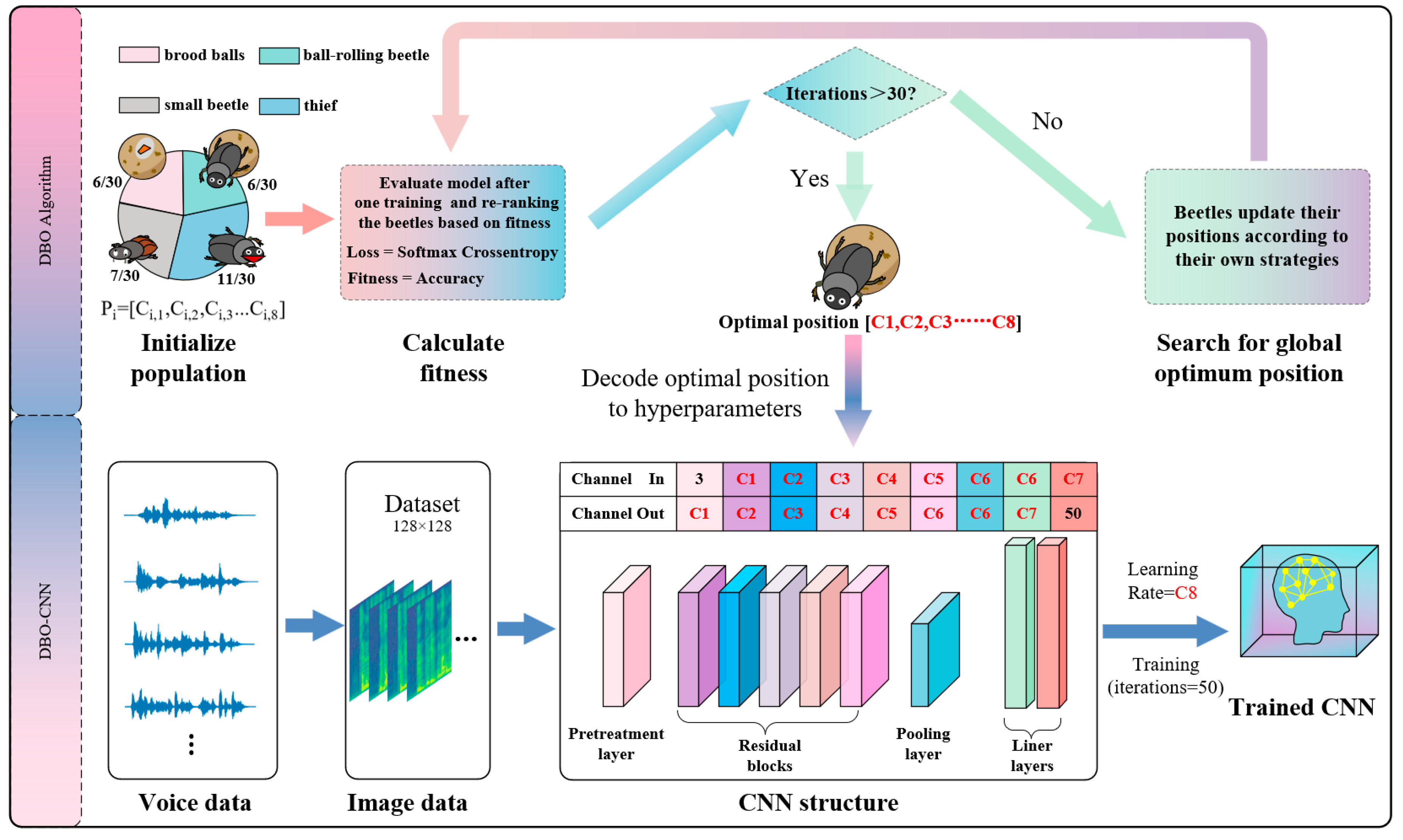
3.4. Optimization Process

ResNet18 has five residual blocks, so the number of output channels or convolution kernel for the five residual blocks needs to be determined. In order to improve the expression ability of the network, an additional hidden layer is added to the full connection layer; thus, its number of neurons needs to be determined. Finally, we need to determine the learning rate in the training process. All hyperparameters and their ranges that need to be optimized for this model are shown in

Table 1. The hyperparameter range of the model.

Layer	Range
preprocessing layer	16~32
residual block 1	32~64
residual block 2	64~128
residual block 3	128~256
residual block 4	256~512
residual block 5	512~1024
extra linear layer	256~512
learning rate	1 × 102~1 × 10−3

. The dimension that beetles need to search is 8.

The process of speaker recognition using DBO-CNN is shown in Figure 5. The position of each beetle is represented by an 8-dimensional vector ${\mathrm{P}}_{\mathrm{i}}({\mathrm{C}}_{\mathrm{i},1},{\mathrm{C}}_{\mathrm{i},2}\dots {\mathrm{C}}_{\mathrm{i},8})$, whose dimension is equal to the number of hyperparameters to be optimized. The calculation method of the fitness value of the beetle is as follows: the beetle’s location parameter is used as the hyperparameter of the model, and only one training is performed after the model is built; at this time, the recognition rate of the model is regarded as the fitness of the beetle at the current position. Then, let each beetle move to a new position according to the strategy in Section 3.3. The above process is called one search. The beetle population is set to 50, and the number of searches is set to 30. After all searches are done, the beetle with the greatest fitness is selected, and its positional parameters represent the best hyperparameters. The model ultimately used in this study will be constructed accordingly. The trained model is obtained after 50 iterations, which reveals the correspondence between spectrogram data and 50 participants. The above optimization and training process can be divided into the following five steps:

• Step I: Divide the data set into a training set and a test set in a ratio of about 8:2
• Step II: Initialize the population to 50 and divide them into different beetle roles according to the fitness ranking. Among them, the proportion of ball-rolling beetles is 6/30(10), the proportion of brood balls is 6/30(10), the proportion of small beetles is 7/30(12) and the proportion of thief beetles is 11/30(18)
• Step III: The beetles search for the optimal hyperparameter group according to their own strategies of position adjustment
• Step IV: Build a convolutional neural network for speaker recognition by using the optimal hyperparameters
• Step V: Evaluate the model on the test set after training.

4. Experiments and Results

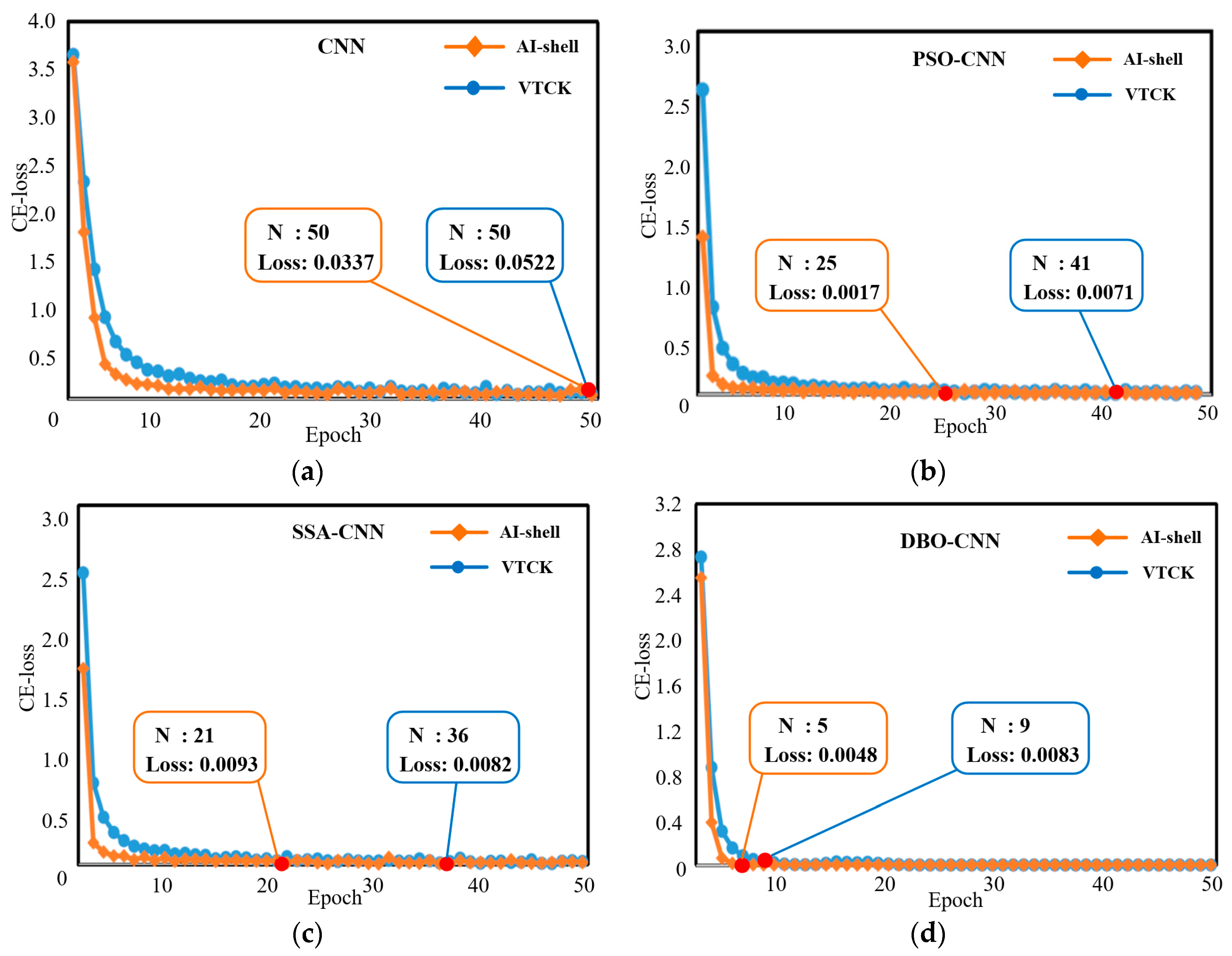
4.1. Hyperparameters Optimization

DBO provides an efficient guide for determining the hyperparameters of CNN; however, it also has some population-related constants to be set. In this study, the constants are used the same as the author of DBO: k = 0.1, b = 0.3, S = 0.5 [34]. The evaluation of the performance of DBO-CNN, PSO-CNN, SSA-CNN, and CNN built by experience is implemented, and their comparison with DBO-CNN is carried out in this paper. During the optimization process, the population and the number of searches were also set to 50 and 30. After iteration, the hyperparameters found by the three algorithms are shown in

Table 2. Hyperparameters searched by different models.

Layer	CNN		PSO-CNN		SSA-CNN		DBO-CNN
	AI-Shell	VTCK	AI-Shell	VTCK	AI-Shell	VTCK	AI-Shell	VTCK
preprocessing layer	32	32	24	30	27	19	21	32
residual block 1	64	64	32	49	54	51	63	43
residual block 2	128	128	117	92	107	75	71	127
residual block 3	256	256	230	239	143	135	256	201
residual block 4	512	512	386	504	424	278	272	256
residual block 5	1024	1024	424	997	904	555	653	512
extra linear layer	512	512	272	403	394	352	259	512
learning rate	1 × 10−2	1 × 10−2	1 × 10−3	1 × 10−3	1 × 10−3	1 × 10−3	1 × 10−3	1 × 10−3

, and the hyperparameters chosen empirically are also listed.

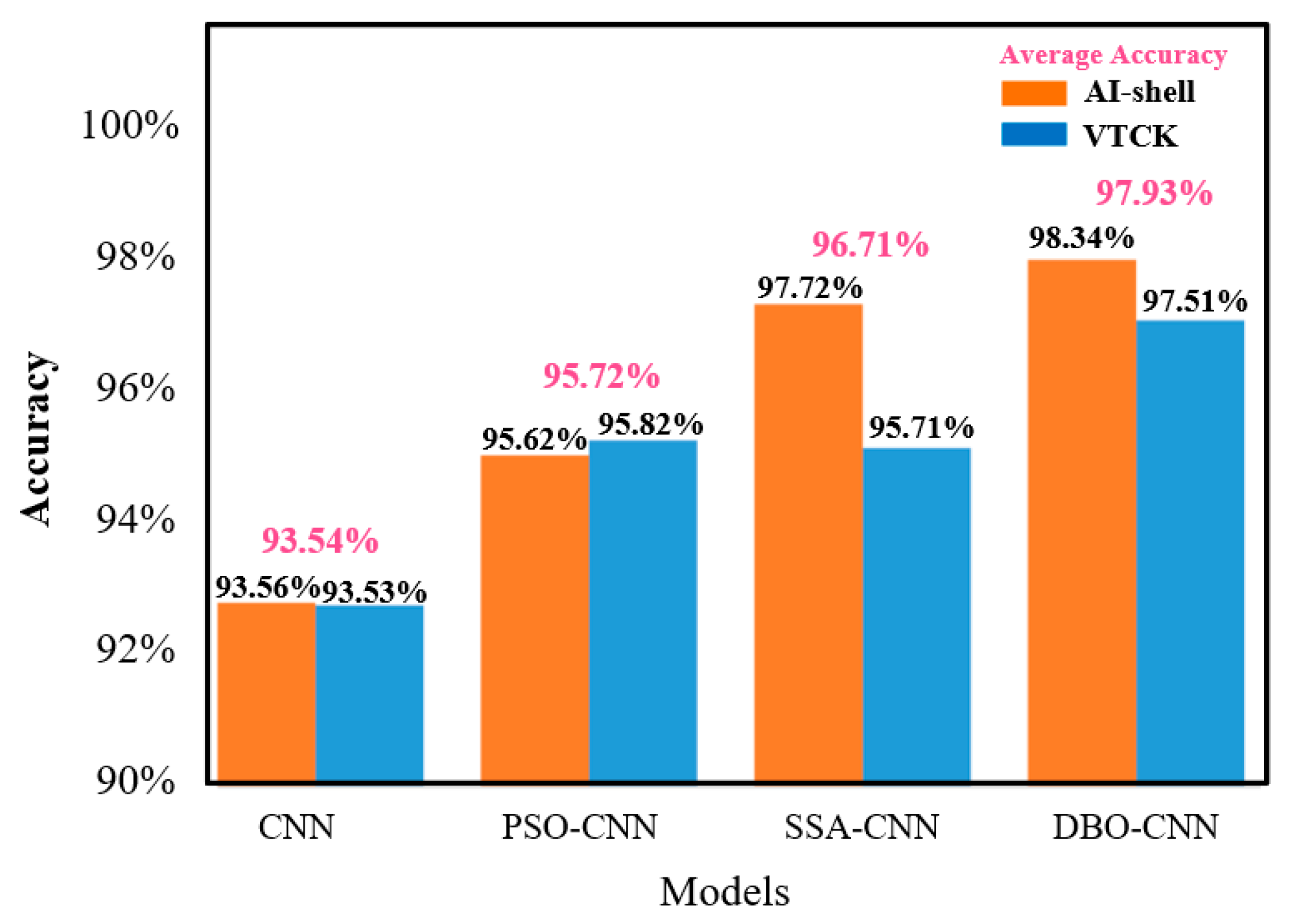
4.2. Recognition Performance

The CNNs using the above four sets of hyperparameters are constructed, and the produced spectrograms are imported into them for training. The loss function is SoftMaxCrossEntropy. The number of iterations is set to 50.

As shown in Figure 6, by 50 iterations on two datasets, the loss of traditional CNN will not decrease to below 0.01, which is the worst among the models. When tested on the AI-shell dataset, DBO-CNN performs the best by reducing losses to below 0.01 after only 5 iterations, PSO-CNN spends 25 iterations, and SSA-CNN spends 21 iterations. It is indicated that DBO significantly improves the training speed of the model. When tested on the VTCK dataset, DBO-CNN also showed the best convergence speed. The evaluation results of the four models on the test set are shown in Figure 7. After the optimization of the intelligent algorithm, the accuracy of the model has been significantly improved. Among them, DBO-CNN has the greatest improvement with an average accuracy rate of 97.93%, followed by SSA-CNN with an accuracy rate of 96.71%, and finally, PSO-CNN with an accuracy rate of 95.72%. It is demonstrated that DBO is indeed superior to traditional intelligent algorithms such as PSO.

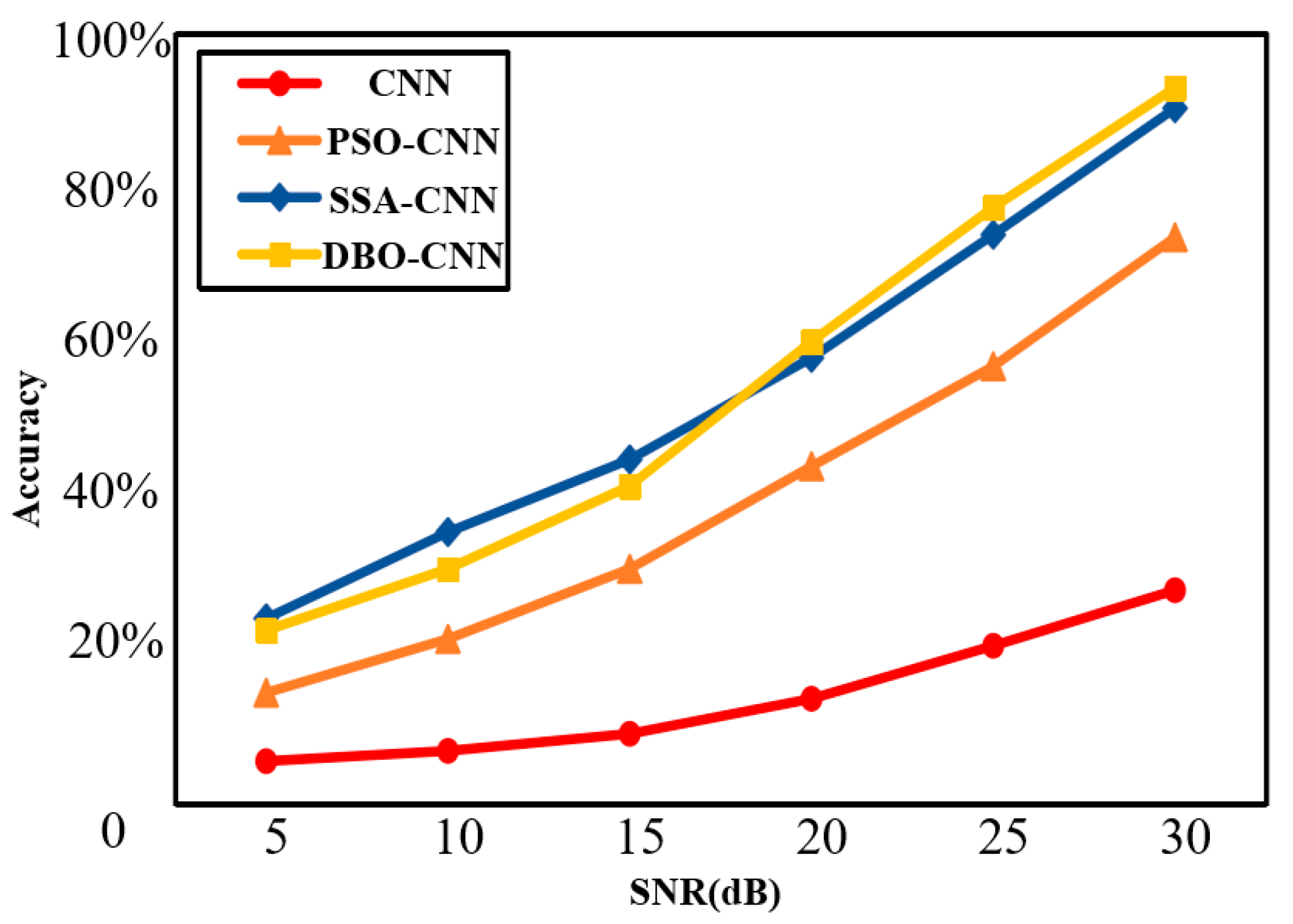
4.3. Noise Resistance Test

Due to environmental noise interference or performance limitations of recording equipment, the effects of the audio are always unsatisfactory. In order to test the anti-interference ability of the model in this environment, some white noise is added to the previous test set data. We tested the performance of the model by different signal-to-noise ratios. As shown in Figure 8, as the proportion of noise increases, the recognition accuracy of all models decreases. The anti-noise ability of the two newer meta-heuristic algorithms is basically the same, and the accuracy is still around 80% in a signal-to-noise ratio environment of 30 dB. Even in a harsh environment of 20 dB, the accuracy of both algorithms is above 50%, which is acceptable. However, the accuracy of particle algorithms and traditional CNN in noisy environments has significantly decreased, and their anti-noise performance is significantly weaker than the new meta-heuristic algorithm.

5. Conclusions and Future Work

A DBO-CNN algorithm has been proposed for speaker recognition in this study and compared with the CNN, PSO-CNN, and SSA-CNN algorithms on a dataset of 50 people. After optimization, the performance of all models has improved. DBO-CNN has better optimization ability. It not only has the fastest convergence speed but also has the highest average accuracy, reaching 97.93%. In terms of anti-interference, DBO-CNN and SSA-CNN have similar performance, and their recognition rates are both above 50% in harsh environments of 20 dB. Based on the results, it demonstrates that the DBO-CNN has greatly improved speaker recognition compared with other optimization algorithms and also illustrates that DBO has enormous potential in optimizing CNN. However, the current work still needs a lot of improvement; for example, the model can only classify the voices of 50 people. Converting sound data into a spectrogram and importing it into the model for inference takes a lot of time.

In future work, we will increase the size of the dataset and the number of speakers that can be identified, consider the problem of cross-domain recognition, and classify and recognize complex data sets containing multi-species sounds. In addition, the use of speaker recognition to discriminate AI-based voice synthesis technology will be the focus of future research and a synthetic approach to measuring the performance of the indexes will be used for speaker recognition [36]. Swarm intelligence is a promising and challenging science subbranch. In 2021, the Nobel Physics Award was partially granted to the work on swarm behavior and intelligence. Meanwhile, new developments from multiple fields are deepening and broadening the cognition of swarm intelligence. For the swarm intelligence method based on bionic computing, some recent biological achievements, such as adaptive mutability [37] and epigenetics [38], are sure to improve the performance of speaker recognition. These sophisticated swarm optimization algorithms will be attempted for speaker recognition. The edge deployment of the proposed model will also be accelerated, especially the design based on FPGA, which will promote the application of machine learning for speaker recognition.

References

1. Thullier, F.; Bouchard, B.; Menelas, B.-A.J. A Text-Independent Speaker Authentication System for Mobile Devices. Cryptography 2017, 1, 16. [Google Scholar] [CrossRef]
2. Gupta, H.; Gupta, D. LPC and LPCC method of feature extraction in Speech Recognition System. In Proceedings of the 2016 6th International Conference—Cloud System and Big Data Engineering (Confluence), Noida, India, 14–15 January 2016; pp. 498–502. [Google Scholar]
3. Chia Ai, O.; Hariharan, M.; Yaacob, S.; Sin Chee, L. Classification of speech dysfluencies with MFCC and LPCC features. Expert Syst. Appl. 2012, 39, 2157–2165. [Google Scholar] [CrossRef]
4. Tripathi, A.; Singh, U.; Bansal, G.; Gupta, R.; Singh, A.K. A Review on Emotion Detection and Classification using Speech. In Proceedings of the International Conference on Innovative Computing & Communications (ICICC) 2020, New Delhi, India, 21–23 February 2020. [Google Scholar]
5. Tiwari, V. MFCC and its applications in speaker recognition. Int. J. Emerg. Technol. 2010, 1, 19–22. [Google Scholar]
6. Bhadragiri, J.M.; Ramesh, B.N. Speech recognition using MFCC and DTW. In Proceedings of the 2014 International Conference on Advances in Electrical Engineering (ICAEE), Vellore, India, 9–11 January 2014; pp. 1–4. [Google Scholar]
7. Nakagawa, S.; Zhang, W.; Takahashi, M. Text-independent speaker recognition by combining speaker-specific GMM with speaker adapted syllable-based HMM. In Proceedings of the 2004 IEEE International Conference on Acoustics, Speech, and Signal Processing, Montreal, QC, Canada, 30 August 2004; pp. 1–81. [Google Scholar]
8. Matsui, T.; Kanno, T.; Furui, S. Speaker recognition using HMM composition in noisy environments. Comput. Speech Lang. 1996, 10, 107–116. [Google Scholar] [CrossRef]
9. Limkar, M.; Rao, B.R.; Sagvekar, V. Speaker Recognition using VQ and DTW. Int. J. Comput. Appl. 2012, 3, 975–8887. [Google Scholar]
10. Keogh, E.; Ratanamahatana, C.A. Exact indexing of dynamic time warping. Knowl. Inf. Syst. 2005, 7, 358–386. [Google Scholar] [CrossRef]
11. Hanifa, R.M.; Isa, K.; Mohamad, S. A review on speaker recognition: Technology and challenges. Comput. Electr. Eng. 2021, 90, 107005. [Google Scholar] [CrossRef]
12. Zheng, R.; Zhang, S.; Xu, B. Text-independent speaker identification using GMM-UBM and frame level likelihood normalization. In Proceedings of the 2004 International Symposium on Chinese Spoken Language Processing, Hong Kong, China, 15–18 December 2004; pp. 289–292. [Google Scholar]
13. Liu, Z.; Wu, Z.; Li, T.; Li, J.; Shen, C. GMM and CNN Hybrid Method for Short Utterance Speaker Recognition. IEEE Trans. Ind. Inform. 2018, 14, 3244–3252. [Google Scholar] [CrossRef]
14. McLaren, M.; Lei, Y.; Scheffer, N.; Ferrer, L. Application of convolutional neural networks to speaker recognition in noisy conditions. In Proceedings of the 15th Annual Conference of the International Speech Communication Association, Singapore, 14–18 September 2014; pp. 1990–9770. [Google Scholar]
15. Abdel-Hamid, O.; Mohamed, A.; Jiang, H.; Penn, G. Applying Convolutional Neural Networks concepts to hybrid NN-HMM model for speech recognition. In Proceedings of the 2012 IEEE International Conference on Acoustics, Speech and Signal Processing (ICASSP), Kyoto, Japan, 25–30 March 2012; pp. 4277–4280. [Google Scholar]
16. Campbell, W.M.; Sturim, D.E.; Reynolds, D.A. Support vector machines using GMM supervectors for speaker verification. IEEE Signal Process. Lett. 2006, 13, 308–311. [Google Scholar] [CrossRef]
17. Wang, S.; Zhao, B.; Du, J. Research on transformer fault voiceprint recognition based on Mel time-frequency spectrum-convolutional neural network. J. Phys. Conf. Ser. 2022, 2378, 12–89. [Google Scholar] [CrossRef]
18. Ashar, A.; Bhatti, M.S.; Mushtaq, U. Speaker Identification Using a Hybrid CNN-MFCC Approach. In Proceedings of the 2020 International Conference on Emerging Trends in Smart Technologies (ICETST), Karachi, Pakistan, 26–27 March 2020; pp. 1–4. [Google Scholar]
19. Chung, J.S.; Nagrani, A.; Zisserman, A. Voxceleb2: Deep speaker recognition. arXiv 2018, arXiv:1806.05622. [Google Scholar]
20. Jagiasi, R.; Ghosalkar, S.; Kulal, P.; Bharambe, A. CNN based speaker recognition in language and text-independent small scale system. In Proceedings of the 2019 Third International conference on I-SMAC (IoT in Social, Mobile, Analytics and Cloud) (I-SMAC), Palladam, India, 12–14 December 2019; pp. 176–179. [Google Scholar]
21. İnik, Ö.; Altıok, M.; Ülker, E.; Koçer, B. MODE-CNN: A fast converging multi-objective optimization algorithm for CNN-based models. Appl. Soft Comput. 2021, 109, 107582. [Google Scholar] [CrossRef]
22. Yoo, J.H.; Yoon, H.I.; Kim, H.G.; Yoon, H.S.; Han, S.S. Optimization of Hyper-parameter for CNN Model using Genetic Algorithm. In Proceedings of the 2019 1st International Conference on Electrical, Control and Instrumentation Engineering (ICECIE), Kuala Lumpur, Malaysia, 25–25 November 2019; pp. 1–6. [Google Scholar]
23. Ishaq, A.; Asghar, S.; Gillani, S.A. Aspect-Based Sentiment Analysis Using a Hybridized Approach Based on CNN and GA. IEEE Access 2020, 8, 135499–135512. [Google Scholar] [CrossRef]
24. Chen, J.; Jiang, J.; Guo, X.; Tan, L. A self-Adaptive CNN with PSO for bearing fault diagnosis. Syst. Sci. Control Eng. 2020, 9, 11–22. [Google Scholar] [CrossRef]
25. Bhuvaneshwari, K.S.; Venkatachalam, K.; Hubálovský, S.; Trojovský, P.; Prabu, P. Improved Dragonfly Optimizer for Intrusion Detection Using Deep Clustering CNN-PSO Classifier. Comput. Mater. Contin. 2022, 70, 5949–5965. [Google Scholar] [CrossRef]
26. Mirjalili, S.; Lewis, A. The whale optimization algorithm. Adv. Eng. Softw. 2016, 95, 51–67. [Google Scholar] [CrossRef]
27. Mirjalili, S.; Mirjalili, S.M.; Lewis, A. Grey wolf optimizer. Adv. Eng. Softw. 2014, 69, 46–61. [Google Scholar] [CrossRef]
28. Xue, J.; Shen, B. A novel swarm intelligence optimization approach: Sparrow search algorithm. Syst. Sci. Control Eng. 2020, 8, 22–34. [Google Scholar] [CrossRef]
29. Peraza-Vázquez, H.; Peña-Delgado, A.; Ranjan, P.; Barde, C.; Choubey, A.; Morales-Cepeda, A.B. A bio-inspired method for mathematical optimization inspired by arachnida salticidade. Mathematics 2021, 10, 102. [Google Scholar] [CrossRef]
30. Xie, Q.; Zhou, W.; Ma, L.; Chen, Z.; Wu, W.; Wang, X. Improved whale optimization algorithm for 2D-Otsu image segmentation with application in steel plate surface defects segmentation. Signal Image Video Process. 2023, 17, 1653–1659. [Google Scholar] [CrossRef]
31. Hou, Y.; Gao, H.; Wang, Z.; Du, C. Improved Grey Wolf Optimization Algorithm and Application. Sensors 2022, 22, 3810. [Google Scholar] [CrossRef] [PubMed]
32. Tuerxun, W.; Xu, C.; Guo, H.; Jin, Z.; Zhou, H. Fault Diagnosis of Wind Turbines Based on a Support Vector Machine Optimized by the Sparrow Search Algorithm. IEEE Access 2021, 9, 69307–69315. [Google Scholar] [CrossRef]
33. Muthuramalingam, L.; Chandrasekaran, K.; Xavier, F.J. Electrical parameter computation of various photovoltaic models using an enhanced jumping spider optimization with chaotic drifts. J. Comput. Electron. 2022, 21, 905–941. [Google Scholar] [CrossRef]
34. Xue, J.; Shen, B. Dung beetle optimizer: A new meta-heuristic algorithm for global optimization. J. Supercomput. 2023, 79, 7305–7336. [Google Scholar] [CrossRef]
35. He, K.; Zhang, X.; Ren, S.; Sun, J. Deep residual learning for image recognition. In Proceedings of the 2016 IEEE Conference on Computer Vision and Pattern Recognition, Las Vegas, NV, USA, 26 June–1 July 2016; pp. 770–778. [Google Scholar]
36. Wang, P.; Zhang, J.; Xu, L.; Wang, H.; Feng, S.; Zhu, H. How to measure adaptation complexity in evolvable systems–A new synthetic approach of constructing fitness functions. Expert Syst. Appl. 2011, 38, 10414–10419. [Google Scholar] [CrossRef]
37. Reilly, N.; Arena1, S.; Lamba, S.; Bartolini, A.; Amodio, V.; Magrì, A.; Novara, L.; Sarotto, I.; Nagel, Z.D.; Piett, C.G.; et al. Adaptive mutability of colorectal cancers in response to targeted therapies. Science 2019, 366, 1473–1480. [Google Scholar]
38. Pan, Z.; Yao, Y.; Yin, H.; Cai, Z.; Wang, Y.; Bai, L.; Kern, C.; Halstead, M.; Chanthavixay, G.; Trakooljul, N.; et al. Pig genome functional annotation enhances the biological interpretation of complex traits and human disease. Nat. Commun. 2021, 12, 5848. [Google Scholar] [CrossRef]
Figure 1. The process of recognizing the speaker.
Applsci 13 09787 g001
Figure 2. Generation process of the spectrogram.
Applsci 13 09787 g002
Figure 3. The CNN architecture.
Applsci 13 09787 g003
Figure 4. The composition of ResNet and the structure of the residual block.
Applsci 13 09787 g004
Figure 5. The process for recognizing speakers by using the optimized DBO.
Applsci 13 09787 g005
Figure 6. Comparison of loss of Four Different CNN Models during Training. (a) The Loss Curve of Traditional CNN, (b) the Loss Curve of PSO-CNN, (c) the Loss Curve of SSA-CNN, and (d) the Loss Curve of DBO-CNN.
Applsci 13 09787 g006
Figure 7. Accuracy of the models CNN, PSO-CNN, SSA-CNN, and DBO-CNN.
Applsci 13 09787 g007
Figure 8. Recognition accuracy of four models by different signal-to-noise ratios.
Applsci 13 09787 g008