Multi-Scale Spatial–Temporal Transformer: A Novel Framework for Spatial–Temporal Edge Data Prediction

Abstract

Spatial–temporal prediction is an important part of a great number of applications, such as urban traffic control, urban traffic management, and urban traffic planning. However, real-world spatial–temporal data often have complex patterns, so it is still challenging to predict them accurately. Most existing spatial–temporal prediction models fail to aggregate the spatial features in a suitable neighborhood during fixed spatial dependencies extraction and lack adequately comprehensive time series analysis for intricate temporal dependencies. This paper proposes a novel model named multi-scale spatial–temporal transformer network (MSSTTN) to deal with intricate spatial–temporal patterns. Firstly, we develop an improved graph wavelet neural network, which learns how to pass the spatial graph signals of different frequency scales to adjust the neighborhood of feature aggregation adaptively. Then, we propose decomposing the time series into local trend-cyclical parts of various scales during time series analysis, making the model capture more reliable temporal dependencies. The proposed model has been evaluated on publicly available real-world datasets. The experimental findings indicate that the proposed model exhibits superior performance compared to conventional techniques including, spatial–temporal transformer (STTNs), GraphWaveNet, and others.

1. Introduction

The rise of intelligent transportation systems (ITSs) [1] has led to the increased importance of traffic prediction in urban management [2,3,4,5]. As a core component of the aforementioned traffic applications, traffic prediction, which is a classical spatial–temporal prediction, has attracted the attention of many researchers. Spatial–temporal prediction mines future trends through learning historical data in time and space. Improving the accuracy of spatial-temporal prediction, especially long-term prediction, is of great significance. However, the intricate spatial–temporal dependencies pose a significant obstacle to achieving accurate spatial–temporal series prediction.

Early mathematical spatial-temporal prediction models make predictions based on statistical methods [6,7,8] failed to deal with the dynamic correlations among variable parts in both the spatial and temporal dimensions. To address the weakness of statistical prediction methods, traditional shallow machine learning methods [9,10] emphasize the linear mapping relation that can better capture the complex inherent laws in spatial-temporal data. However, they ignore the sequence connections that perform poorly in both spatial and temporal dependencies extraction. In contrast, deep learning methods perform better in complex spatial-temporal correlation capturing.

Most existing spatial–temporal deep learning models cannot capture the fixed spatial dependencies in neighborhoods with an appropriate size and ignore multi-scale important temporal attributes, leading to a failure to match the accurate spatial correlations. To overcome the limitations, we propose the multi-scale spatial–temporal transformer network (MSSTTN) to extract information of various scales to improve spatial–temporal prediction. First, we introduce and improve the GWNN to capture multi-scale fixed spatial dependencies using different scaling parameters. Second, series decomposition and an Auto-Correlation mechanism are introduced to analyze the historical temporal patterns. Moreover, we propose to decompose the time series into different local trends, which facilitates the acquisition of temporal information at multiple scales and augments the precision of capturing temporal dependencies. The contributions of the paper are summarized as follows:

• We introduced and improved the GWNN to the spatial–temporal transformer network. By making the scaling parameter learnable, the improved GWNN can aggregate the spatial features adaptively that strengthens the fixed spatial dependencies extraction.
• We proposed a novel series multi-scale decomposition to enhance time series analysis by trend-cyclical parts at various scales, making MSSTTN powerful in capturing long-term dependencies.
• We conducted experiments on three datasets, PEMS03, PEMS04, and PEMS08 [11], and the results demonstrate the superiority of MSSTTN in long-term spatial–temporal prediction.

In the rest of this paper, Section 2 discusses the related work of spatial–temporal prediction. The architecture of MSSTTN is constructed in Section 3. Section 4 describes the experimental settings, conducts a series of experiments, and analyzes the results. Finally, the conclusions are discussed in Section 5.

2. Related Work

In the realm of spatial–temporal series prediction, the two primary categories of methods are statistical methods and machine learning methods.

Statistical prediction methods such as vector autoregressive (VAR) [6], Kalman filtering model (KM) [7], and k-nearest neighbor (KNN) [8] can be used for the development of suitable mathematical models. However, they are limited in their capacity to extract dynamic and fixed spatial dependencies. As an upgraded version of autoregressive (AR) [12], the VAR achieves spatial–temporal series prediction by constructing multiple equations to calculate the dynamic relationship of all endogenous variables. However, the VAR model’s limitations are evident in its inability to effectively predict spatial–temporal series due to it cannot leverage the dynamic dependencies among multiple variables. Anyway, statistical prediction methods often encounter challenges in making long-term predictions and are unable to capture dynamic spatial–temporal dependencies.

To address the weakness of these statistical prediction methods, traditional shallow machine learning methods, such as support vector machine (SVM) [9] and random forest [10], can better capture inherent laws but not for multivariate prediction because they emphasize nonlinear mapping relationships rather than sequence connections. As highly complex systems, recurrent neural networks (RNNs) [13] and their variations, including long short-term memory (LSTM) [14] and gated recurrent unit (GRU) [15], are capable of capturing temporal correlations. The diffusion convolutional recurrent neural network (DCRNN) [16] is a model that integrates diffusion convolution and recurrent neural networks (RNNs) to capture spatial–temporal dependencies to make a prediction. Tian et al. [17] proposed the CNN-LSTM model by fusing the LSTM and convolutional neural network (CNN), achieving great performance in short-term prediction. Wang et al. [18] proposed multiple CNN models for periodic multivariate time prediction. Nevertheless, limited by convolution kernel size, it is difficult to capture long-term temporal dependencies with CNNs. The proposal of a self-attention mechanism was verified as a powerful tool for long-term prediction. Spatial–temporal transformer networks (STTNs) [19] adopts self-attention to model the temporal dependencies and achieve competitive results. The attention-based spatial–temporal graph neural network (ASTGNN) [20] embeds CNN in self-attention to enable temporal dynamics and obtain global receptive fields that significantly improve long-term prediction accuracy. LogTrans [21] adopts local convolution and LogSparse attention to reduce the complexity to $O\left(L{\left(logL\right)}^2\right)$. Informer [22] achieves complexity $O\left(LlogL\right)$ by introducing KL-divergence-based ProbSparse attention. Autoformer [23] presents series decomposition and utilizes a custom-designed Auto-Correlation mechanism that dramatically improves long-term prediction accuracy.

Spatial dependencies modeling is also a significant part of spatial–temporal prediction. The deep multi-view spatial–temporal network (DMVST-Net) [24] applies local CNNs to capture the local characteristics of regions about the neighbors of each node. However, the CNNs [25] cannot be adaptive to graph-based spatial data. Subsequent to the emergence of graph neural networks (GNNs) [26], graph convolution networks such as ChebNet [27] were proposed later. The temporal graph convolutional network (T-GCN) [28] extracts spatial–temporal dependencies simultaneously through combining the GCN [29] with GRU. Spatio-temporal graph convolutional networks (STGCN) [30] develops a complete convolutional structure composed of the GCN and CNN that replaces convolutional and recurrent units and outperformed the baselines. STTNs introduces ChebNet to extract fixed spatial dependencies.

Nevertheless, it is challenging for GCNs to deal with hidden and dynamic spatial dependencies. GraphWaveNet [31] learns a self-adaptive adjacent matrix for hidden spatial dependencies. ASTGNN [20] designs a dynamic graph convolution net (DGCN) for dynamic dependencies. For calculating spatial correlations at both local and global scales, the utilization of an attention mechanism is prevalent in capturing dynamic spatial dependencies. Spatial–temporal prediction models, such as attention-based spatial–temporal graph convolutional network (ASTGCN) [32] and STTNs, adopt attention mechanisms for dynamic spatial dependencies. Meta graph transformer (MGT) [33] employs a multi-graph with a self-attention mechanism that achieves outstanding performance. ASTGCN [32] applies spatial–temporal attention and spatial–temporal CNNs to make a prediction. STTNs proposes a spatial transformer structured by a self-attention layer and a ChebNet to extract the dynamic and fixed spatial dependencies simultaneously.

As mentioned before, GCNs are extensively utilized in spatial–temporal prediction. Bruna et al. [34] adopt spectral CNN to implement the convolution on graph by graph Fourier transform. For lacking enough flexibility on feature aggregation, Xu et al. [35] proposed graph wavelet neural network (GWNN) by substituting the graph Fourier basis with the graph wavelet basis, which results in feature aggregation within a particular neighborhood range.

3. Methodology

In this section, we describe the preliminaries and propose the multi-scale spatial–temporal transformer network (MSSTTN). Specifically, we analyze the MSSTTN by showing the overall architecture at first and then elaborating on the main components of the model: spatial transformer and temporal autoformer.

3.1. Preliminaries

We use the graph $G=(V,E,A)$ to describe the spatial topological network. V denotes the set of nodes which represent the spatial–temporal data collectors, such as traffic sensors, meteorological observation stations. $\left|V\right|$ is the quantity of nodes, E denotes the set of edges in the spatial networks, and $\left|E\right|$ is the quantity of edges. $A\in R^{N\times N}$ is the adjacent matrix of the spatial networks. ${\mathcal{X}}_t=\left({\mathcal{X}}_{t,1},{\mathcal{X}}_{t,2},\dots ,{\mathcal{X}}_{t,N}\right)\in R^{N\times C}$ represents the features of every node in the spatial graph at time t, where ${\mathcal{X}}_{t,v}\in R^C$ is the feature vector of node v at time t, and C is the quantity of features.

The spatial–temporal prediction is defined as follows: given the historical spatial–temporal matrices $\mathcal{X}=\left({\mathcal{X}}_{t-T_h+1},\right.\left.{\mathcal{X}}_{t-T_h+2},\dots ,{\mathcal{X}}_t\right)\in R^{N\times T_h\times C}$ from the past $T_h$ time slices, the task is to predict the sequence of future spatial–temporal matrices $\mathcal{Y}=({\mathcal{X}}_{t+1},{\mathcal{X}}_{t+2},\dots ,{\mathcal{X}}_{t+T_p})\in R^{N\times T_p\times C}$ over the next $T_p$ time slices.

3.2. Overall Architecture

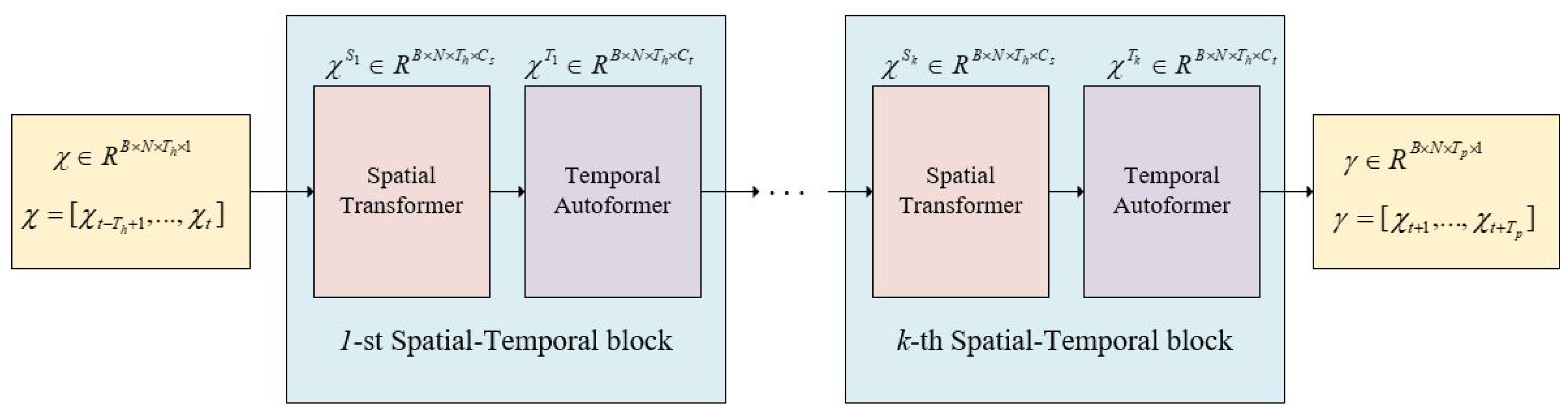
MSSTTN is improved based on STTNs [19], which is structured by stacked spatial–temporal blocks (ST-Blocks). Each of the ST-Blocks are comprised of a spatial transformer and a temporal transformer. The spatial transformer extracts the dynamic spatial dependencies using self-attention mechanism and fixed dependencies using a GCN layer. For long-range temporal dependencies, the temporal transformer employs self-attention mechanism to utilize more information in the time series history. In addition, MSSTTN makes multi-step predictions directly that alleviate the propagated error.

Inspired by STTNs [19], MSSTTN learns the complicated spatial and temporal dependencies by constructing a series of spatial–temporal blocks in which every block contains both a spatial and temporal module. The comprehensive structure is presented in Figure 1. The spatial–temporal block comprises a spatial transformer and temporal autoformer that enable the extraction of both spatial and temporal dependencies. After the extraction operations from the stacked spatial–temporal blocks, the model makes the prediction using the last block. We use ${\mathcal{X}}^i\in R^{B\times N\times T_h\times C_s}$ and ${\mathcal{Y}}^i\in R^{B\times N\times T_h\times C_t}$ to denote the input and output of the i-th spatial–temporal block. The input to the first spatial–temporal block ${\mathcal{X}}^1=\left({\mathcal{X}}_{t-h+1},{\mathcal{X}}_{t-h+2},\dots ,{\mathcal{X}}_t\right)\in R^{B\times N\times T_h\times 1}$ is the historical spatial–temporal data, where B denotes the batch size. Then, the k spatial–temporal blocks will be used to extract spatial–temporal dependencies from ${\mathcal{X}}^1$. For the i-th spatial–temporal block, the input ${\mathcal{X}}^i$ is equal to ${\mathcal{Y}}^{i-1}$. ${\mathcal{X}}^{S_i}$ and ${\mathcal{X}}^{T_i}$ are the spatial and temporal dependencies extraction results of the spatial transformer and temporal autoformer in the i-th spatial–temporal block. Due to ${\mathcal{X}}^{S_i}$ being the input of the temporal autoformer of the i-th spatial–temporal block, ${\mathcal{X}}^{T_i}$ also contains the spatial dependencies extraction results. The output of the i-th spatial–temporal block can be described as ${\mathcal{Y}}^i={\mathcal{X}}^{T_i}$. The prediction results can be described as $\mathcal{Y}=Conv\left({\mathcal{Y}}^k\right)\in R^{B\times N\times T_p\times 1}$, where $Conv\left(\right)$ is a convolution layer and k denotes the number of spatial–temporal blocks. By utilizing stacked spatial–temporal blocks, the MSSTTN captures the spatial–temporal dependencies and then makes predictions in the last block.

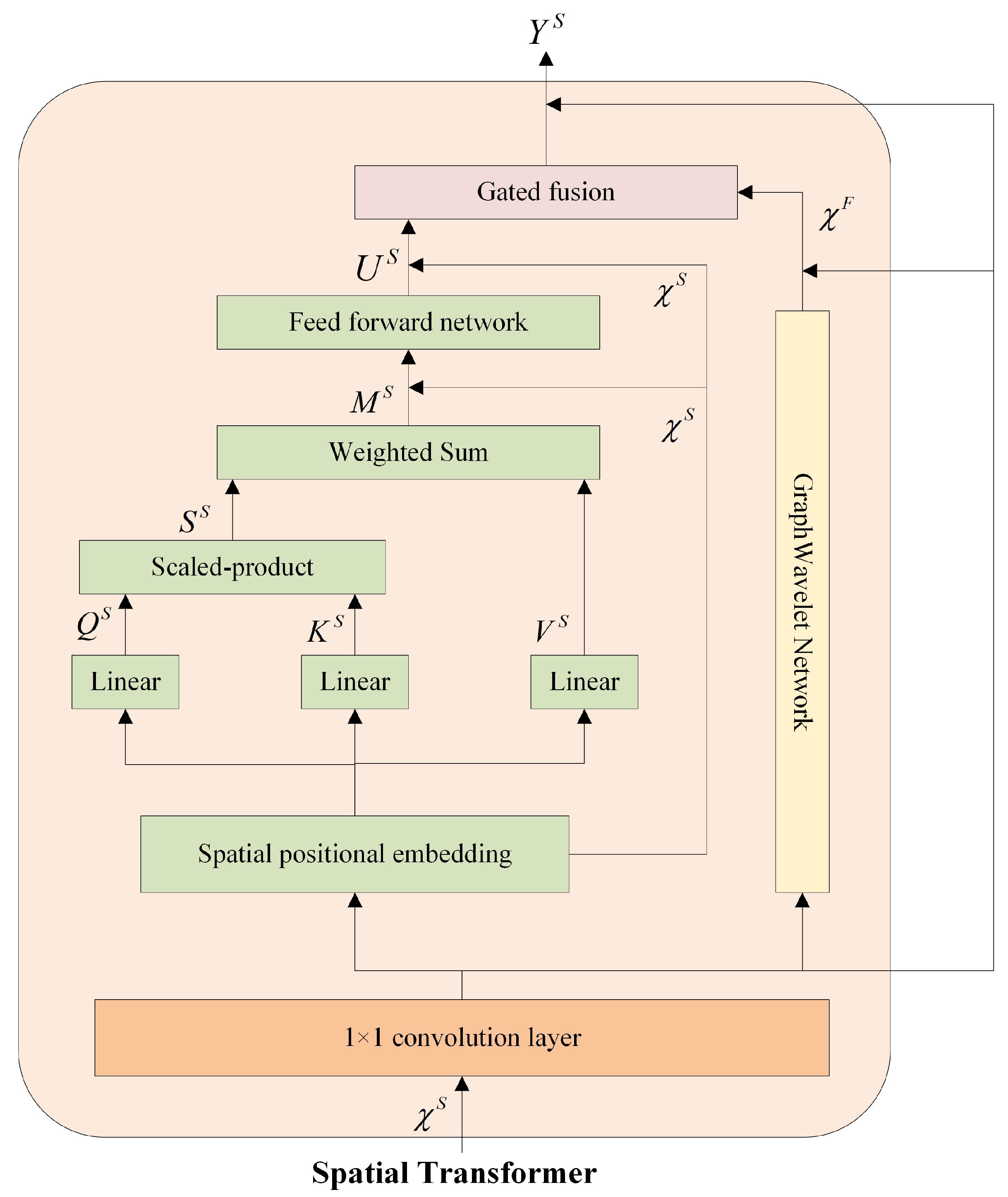
3.3. Spatial Transformer

We employ a self-attention layer to model the dynamic spatial dependencies. Furthermore, we adopt and improve the GWNN to replace the GCN to model the fixed spatial dependencies. The spatial transformer consists of the self-attention layer and improved GWNN. As illustrated in Figure 2, the input features of the spatial transformer will be mapped to a latent high-dimensional subspace by a $1\times 1$ convolution layer and then be utilized by the self-attention layer and the improved GWNN as the basis for computation.

3.3.1. Self-Attention Layer

As mentioned before, the self-attention mechanism is effective in capturing dynamic spatial dependencies. During the calculating process, the sizes of the queries, keys, and values are identical. We use a learnable linear function to map each node to latent high-dimensional subspaces $Q^S$, $K^S$, $V^S$ and then compute the spatial dependencies $S^S$:

$$S^S=softmax\left(\frac{Q^S{\left(K^S\right)}^T}{\sqrt{d_k^S}}\right)$$

(1)

After obtaining the spatial dependencies, we can obtain the updated spatial features $M^S$ using the following formulation:

$$M^S=S^S{V}_S$$

(2)

In addition, a multi-head attention mechanism can be adopted to learn different dynamic spatial dependencies by projecting the input features to various query, key, and value subspaces.

3.3.2. Improved Graph Wavelet Neural Network

Early works of convolution on graphs tended to utilize graph Fourier transform as a means of projecting graph signals into the spectral domain. The technique relies on the eigenvectors of the Laplacian matrix to facilitate the aggregation of signals on the graph. In the graph Fourier transform, the convolution operation can be described as [27]:

$$x{\ast }_{g}y=U\left(\left(U^{T}y\right)\odot \left(U^{T}x\right)\right)$$

(3)

where x denotes the features on graph, ${\ast }_g$ denotes the convolution operator, y denotes the convolution kernel, ⊙ denotes the element-wise Hadamard product, and U denotes the eigenvectors of the Laplacian matrix. Subsequently, it is feasible to replace $U^{T}y$ by a diagonal matrix $g_{\theta }$ and ⊙ by matrix multiplication. So we rewrite Equation (3) as $U{g}_{\theta }{U}^{T}x$. Many kinds of spectral graph convolution neural networks (e.g., ChebNet, GCN) are based on this formulation. STTNs adopts ChebNet to extract the fixed spatial dependencies.

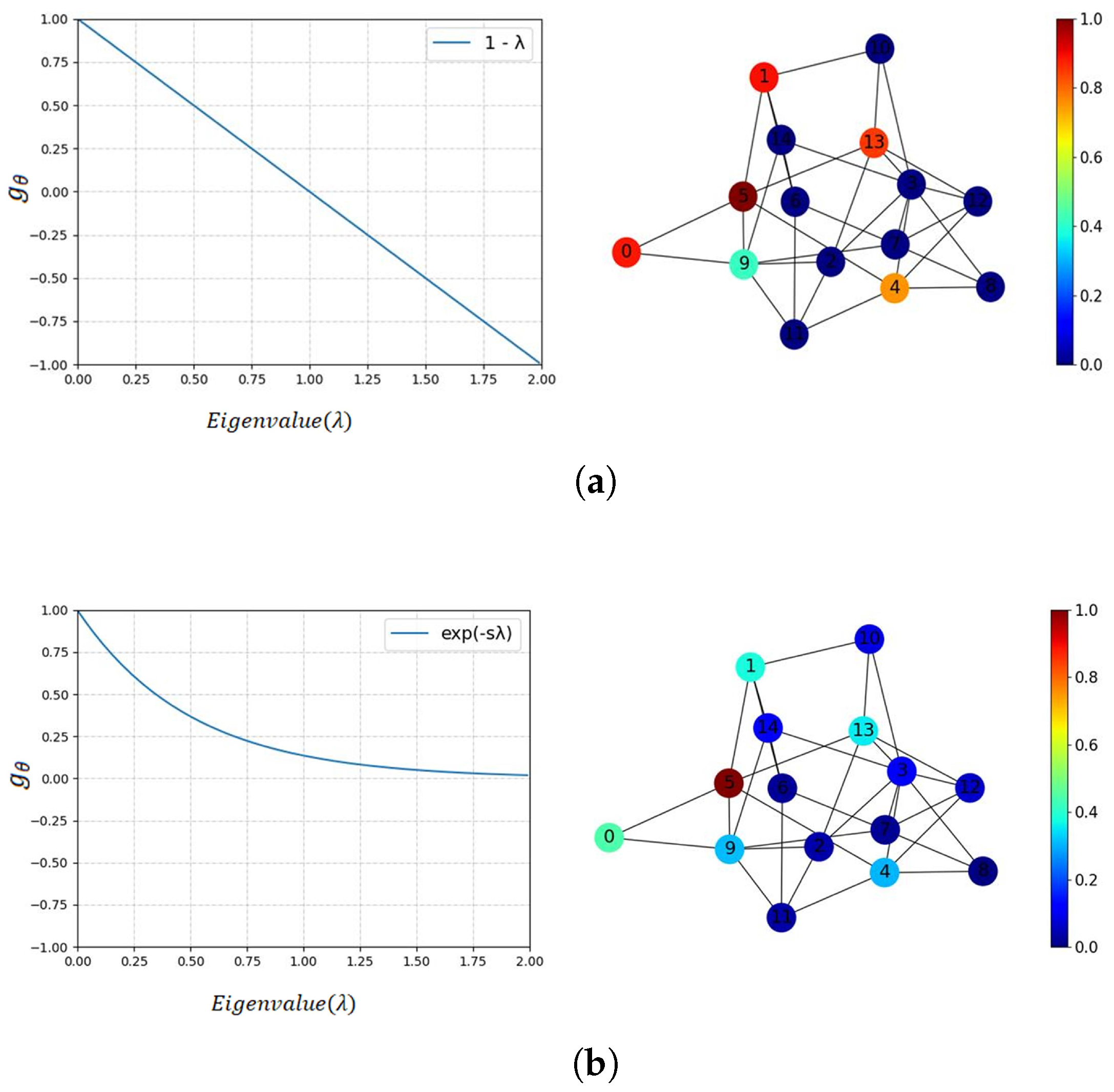
Xu et al. pointed out that graph convolution based on Fourier transform suffers from a restriction in graph flexibility that hinders the ability to establish suitable convolution on the graph. Thus, they proposed the GWNN, which aggregates features not only locally but flexibly. Taking the GCN (a simplified version of ChebNet) as an example, the GCN aggregates the graph signals via a Laplacian renormalization trick: ${\tilde{D}}^{-\frac{1}{2}}A{\tilde{D}}^{-\frac{1}{2}}$, where $\tilde{A}=A+I_N$, ${\tilde{D}}_{ii}={\sum }_{j=0}^N{\tilde{A}}_{ij}$, thus, its graph signal passing process can be described as:

$$U(1-\mathrm{\Lambda })U^T$$

(4)

where U is the matrix of eigenvectors of the Laplacian matrix $L=I_N-{\tilde{D}}^{-\frac{1}{2}}A{\tilde{D}}^{-\frac{1}{2}}$ and $\mathrm{\Lambda }$ is the diagonal matrix of eigenvalues. The signal passing can be described as $1-\lambda$ in the spectral domain so that it is fixed in the first-order neighborhood, as shown in Figure 3a [35].

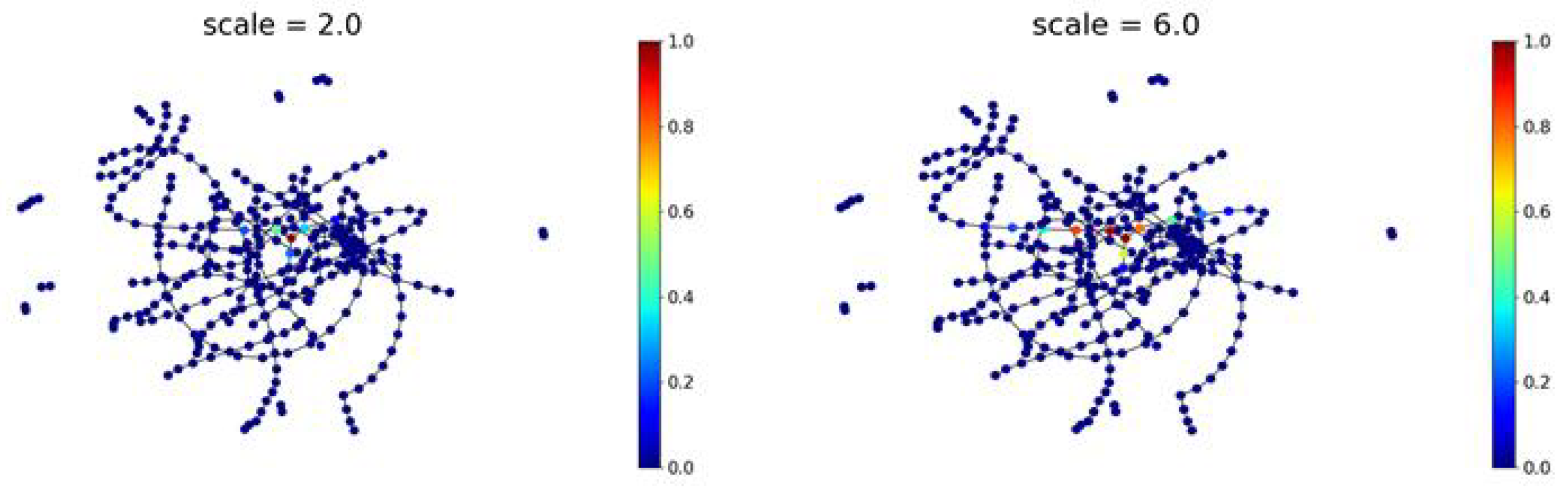
In the present study, we adopt the GWNN to extract the fixed spatial dependencies and improve it by making the scaling parameter “s” learnable, enabling multi-scale graph signal passing, as shown in Figure 4. Analogous to the graph Fourier transform, GWNN projects graph signals into the spectral domain by a set of graph wavelet basis. The graph wavelet basis are defined as ${\psi }_s=\left({\psi }_{s1},{\psi }_{s2},\dots ,{\psi }_{sn}\right)$, where ${\psi }_{si}$ is equivalent to a signal on a graph diffused away from the node i, and s is the scaling parameter of the graph wavelets [35]. ${\psi }_{si}$ can be obtained using the following formulation:

$${\psi }_s=U{G}_s{U}^T$$

(5)

where $G_s=diag\left(g(s{\lambda }_1,s{\lambda }_2,\dots ,s{\lambda }_n)\right)$ is the scaling matrix and $g\left(s{\lambda }_i\right)=e^{s{\lambda }_i}$, ${\lambda }_i$ is the eigenvalue of the Laplacian matrix. Meanwhile, ${\psi }_s^{-1}$ can be obtained by replacing $g\left(s{\lambda }_i\right)$ with $g(-s{\lambda }_i)$ corresponding to a heat kernel [36]. Otherwise, ${\psi }_s$ and ${\psi }_s^{-1}$ can be efficiently calculated using a Chebyshev polynomials approximation [35,37]. By adjusting the scaling parameters, the neighborhood of feature aggregation can expand or shrink flexibly, as shown in Figure 3b.

With graph wavelet bases, Equation (3) can be replaced by:

$$x{\ast }_{g}y={\psi }_s(\left({\psi }^{-1}y\right)\odot {\psi }^{-1}x))$$

(6)

The formulation of a GWNN layer is:

$$X^{m+1}=h\left({\psi }_s{F}^m{\psi }^{-1}{X}^{m}W\right)$$

(7)

where $w\in R^{d_m\times d_m+1}$ is the learnable weight matrix for feature transformation, $F^m$ is the diagonal matrix for the graph convolution kernel, and h is a nonlinear activation function.

The neighborhood of the original GWNN is static during the learning process. We propose a new learnable method to adjust the scaling parameter, and it assign special weights for graph signals with multi-scale frequencies. This method process feature aggregation in an adaptive neighborhood in the spatial domain.

Inspired by the self-adaptive adjacent matrix of GraphWaveNet [31], we make the scaling parameter learnable. During the learning process, the model can adjust the scaling parameter adaptively so that the improved GWNN can assign the weights on graph signals of frequencies of multi-scale as appropriately as possible. To learn the scale parameter stably, we use two learnable vectors $v_1$ and $v_2$ to obtain it:

$$s=v_1\times v_2$$

(8)

Through the learnable scaling parameter, the GWNN can explore multi-scale graph signals propagation and learn the most suitable feature aggregation scale. In this paper, we use a two-layer improved GWNN to capture the fixed spatial dependencies.

3.4. Temporal Autoformer

Compared with the self-attention mechanism, autoformer performs better in long-term dependencies capturing by adopting series decomposition and the period-based Auto-Correlation mechanism. So we introduce and improve the framework of autoformer to extract the temporal dependencies.

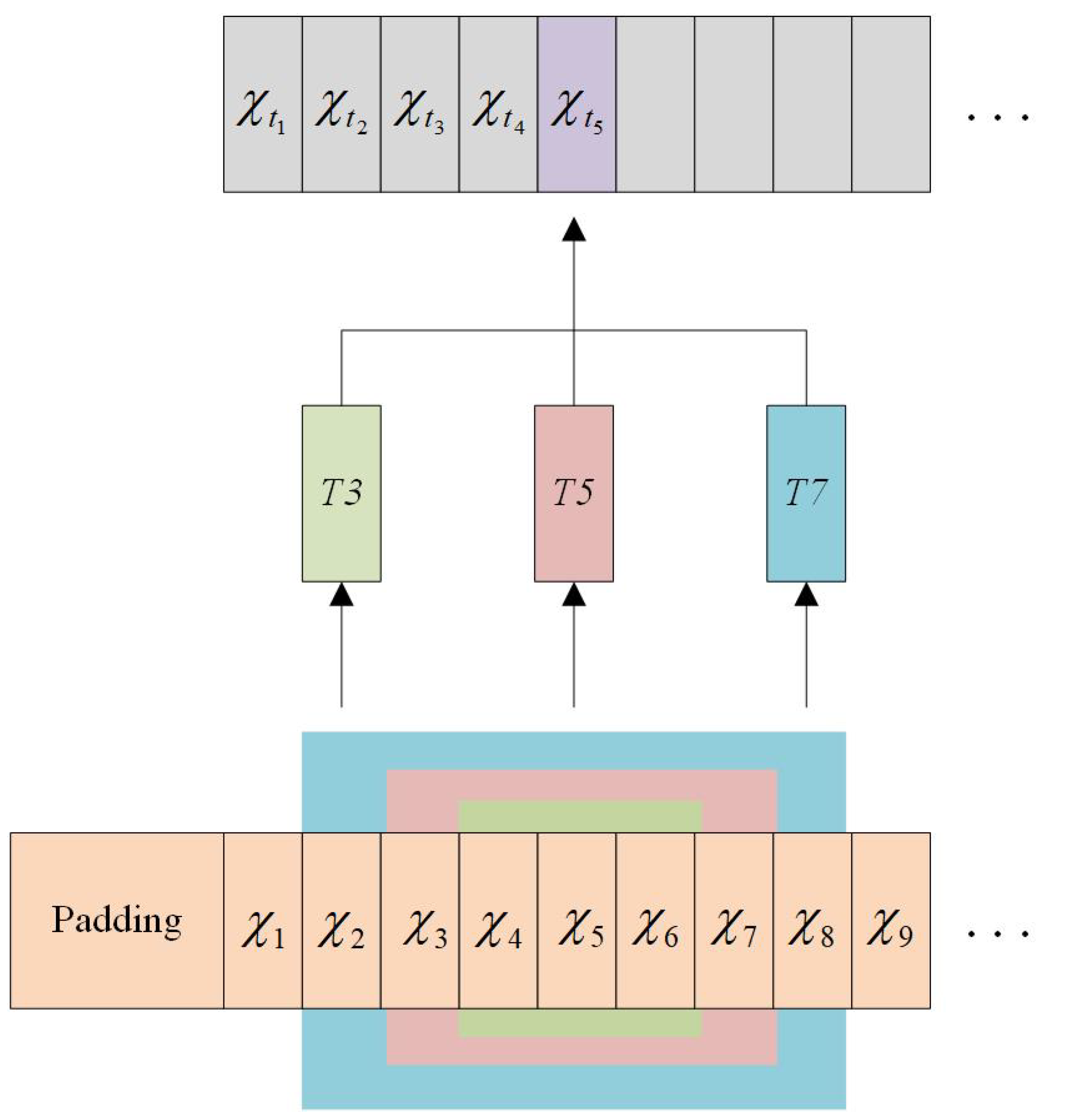
3.4.1. Series Multi-Scale Decomposition

The series decomposition block is an intrinsic operation of autoformer [23], which uses the moving average technique to mitigate cyclic fluctuations and accentuate prolonged patterns. Suppose that there is an input series $\mathcal{X}\in R^{L\times d}$, the original series decomposition can be described as:

$$\begin{array}{cc}\hfill {\mathcal{X}}_t=& \hfill AvgPool\left(Padding\right(\mathcal{X}),k)\hfill \\ \hfill {\mathcal{X}}_s=& \hfill \mathcal{X}-{\mathcal{X}}_t\hfill \end{array}$$

(9)

where ${\mathcal{X}}_t$, ${\mathcal{X}}_s$ refer to the extracted trend-cyclical and seasonal part, respectively, and k denotes the kernel size of the $Avgpool(•)$ operation. The original series decomposition in autoformer only utilizes a single kernel to extract the trend-cyclical part of the time series. So the series decomposition can only be aware of a certain fixed local trend and the series analysis may be inadequate. In this paper, we propose multi-scale decomposition, which can analyze the series in a multi-scale manner. As shown in Figure 5, the series is decomposed into various sized windows with different scales 3, 5, and 7, so that the series decomposition can be analyzed at various scales. Then, the formulation can be redefined as:

$$\begin{array}{cc}\hfill {\mathcal{X}}_t=& \hfill \frac{1}{\left|K\right|}\sum _{k\in K}^{}AvgPool(Padding\left(\mathcal{X}\right),k)\hfill \\ \hfill {\mathcal{X}}_s=& \hfill \mathcal{X}-{\mathcal{X}}_t\hfill \end{array}$$

(10)

where K is the set of various scales of the average pooling windows, and $\left|K\right|$ is the size of K. We use ${\mathcal{X}}_t,{\mathcal{X}}_s=MultiSeriesdecomp(\mathcal{X},K)$ to summarize Equation (10).

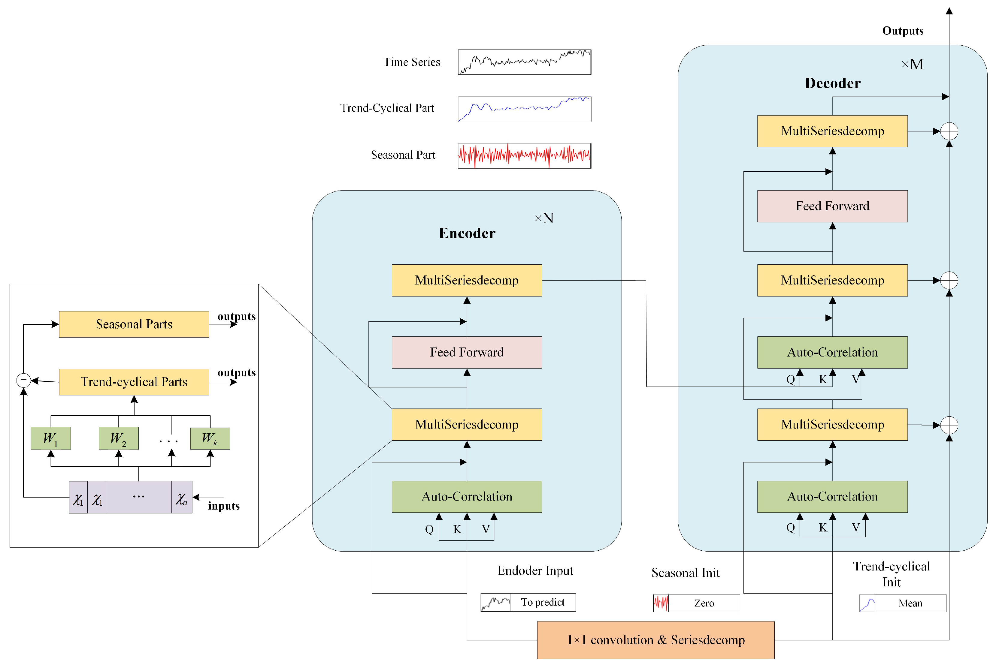
3.4.2. The Overall Architecture of Improved Autoformer

The architecture of improved temporal autoformer is shown in Figure 6 [23]. It is obvious that the temporal autoformer adopts the encoder–decoder structure. For the encoder, the inputs are the processed features in the past I time steps ${\mathcal{X}}_{en}\in R^{B\times I\times d_{model}}$. For the decoder, the inputs contain both the seasonal and trend-cyclical parts of the processed features ${\mathcal{X}}_{ens},{\mathcal{X}}_{\mathit{des}}\in R^{B\times \left(\frac{I}{2}+O\right)\times d_{\mathit{model}}}$. O represents the future length. The details are:

$$\begin{array}{cc}\hfill {\mathcal{X}}_{ent},{\mathcal{X}}_{ens}=& \hfill MultiSeriesdecomp\left({\mathcal{X}}_{en},K\right)\hfill \\ \hfill {\mathcal{X}}_{des}=& \hfill Concat\left({\mathcal{X}}_{ens},{\mathcal{X}}_0\right)\hfill \\ \hfill {\mathcal{X}}_{det}=& \hfill Concat\left({\mathcal{X}}_{ent},{\mathcal{X}}_{Mean}\right)\hfill \end{array}$$

(11)

where ${\mathcal{X}}_0\in R^{O\times d_{model}}$ are the placeholders filled with 0 and ${\mathcal{X}}_{Mean}\in R^{O\times d_{model}}$ are the placeholders populated with the mean values of ${\mathcal{X}}_{en}$.

Both encoder and decoder consist of Auto-Correlation, multi-scale series decomposition, and feed forward networks. Auto-Correlation mechanism employs the connection of sub-series exhibiting similar characteristics through the application of time delay aggregation. The encoder only retains the seasonal part after multi-scale series decomposition. The equation denoting the formulation of the l-th encoder layer can be expressed as ${\mathcal{X}}_{en}^l=Encoder\left({\mathcal{X}}_{en}^{l-1}\right)$, where N represents the total number of encoder layers. The decoder is composed of an accumulation structure to handle multi-scale trend-cyclical components, as well as a stacked Auto-Correlation mechanism to address seasonal components. Extracting temporal trend features at different scales through automatic multi-scale series decomposition, the model can obtain more comprehensive temporal information, then strengthen the ability of encoders and decoders to extract temporal dependencies of different scales and achieve multi-scale temporal feature fusion. Assuming the existence of M decoder layers, the formulation of the l-th decoder layer can be succinctly summarized by ${\mathcal{X}}_{de}^M,{\mathcal{T}}_{de}^M=Decoder({\mathcal{X}}_{de}^{l-1},{\mathcal{X}}_{en}^N)$. Then, the output of the decoder can be obtained by:

$${\mathcal{X}}_o={\mathcal{W}}_{\mathcal{S}}\ast {\mathcal{X}}_{de}^M+{\mathcal{W}}_{\mathcal{T}}\ast {\mathcal{T}}_{de}^M$$

(12)

where ${\mathcal{W}}_{\mathcal{S}}$ and ${\mathcal{W}}_{\mathcal{T}}$ is the weight matrix for seasonal and trend-cyclical components, respectively.

4. Experiment

In this section, we evaluate the newly proposed MSSTTN model with three real-world spatial–temporal datasets, and then compare its performance with classic models. Furthermore, we conduct ablation experiments to validate the effectiveness of the improvements in MSSTTN.

4.1. Datasets

The MSSTTN model is assessed on real-world datasets, namely, PEMS03, PEMS04, and PEMS08. These three traffic datasets pertain to the flow of highway traffic and was procured from the PeMS (performance measurement system) of the California Department of Transportation [11]. The datatype of the datasets is traffic flow, and the flow data of each dataset were collected every five minutes. The number of sensors and the time range are depicted in

Table 1. Dataset descriptions.

Dataset	Number of Sensors	Time Range
PEMS03	358	1 September 2018–30 November 2018
PEMS04	307	1 January 2018–28 February 2018
PEMS08	170	1 July 2016–31 August 2016

. The road topology information will be represented by an adjacency matrix in the experiments.

4.2. Metrics and Baselines

The evaluation metrics we applied for the performance of the models were mean absolute error (MAE), mean absolute percentage error (MAPE), and root mean square error (RMSE). Suppose that $x_1,x_2,\dots ,x_N$ are the actual values and ${\widehat{x}}_1,{\widehat{x}}_2,\dots ,{\widehat{x}}_N$ are the corresponding prediction values. The formulations of MAE, MAPE, and RMSE are as follows:

$$\begin{array}{cc}\hfill MAE(x,\widehat{x})=& \hfill \frac{1}{N}\sum _{i\in [1,N]}^{}|x_i-{\widehat{x}}_i|\hfill \\ \hfill MAPE(x,\widehat{x})=& \hfill \frac{1}{N}\sum _{i\in [1,N]}^{}\left|\frac{x_i-{\widehat{x}}_i}{x_i}\right|\hfill \\ \hfill RMSE(x,\widehat{x})=& \hfill \sqrt{\frac{1}{N}\sum _{i\in [1,N]}^{}{(x_i-{\widehat{x}}_i)}^2}\hfill \end{array}$$

(13)

To conduct the comparison experiments, we selected the following proposed models:

• FC-LSTM. A network that combines long- and short-term memory networks with full connection [38].
• STGCN. Spatio-temporal graph convolutional network, a network that integrates graph convolution with one-dimensional convolutional units [30].
• DCRNN. Diffusion convolutional recurrent neural network, a network that integrates an RNN with diffusion convolution [16].
• ASTGCN. Attention-based spatio-temporal graph convolutional network, a network that adopts spatio-temporal attention for spatial–temporal prediction [32].
• GraphWaveNet. A network that proposes an adaptive adjacency matrix with 1-D diffusion convolution in graph convolution [31].
• STTNs. Spatial–temporal transformer network, a network which is based on the self-attention mechanism and makes prediction by stacked spatial–temporal blocks [19].
• ASTGNN. Attention-based spatial–temporal graph neural network, a network that adopts dynamic GCN and a trend-aware attention mechanism [20].
• FOGS. First-order gradient supervision, a spatial–temporal model that utilizes first-order gradients to train and a learning-based spatial–temporal correlation graph to make predictions [39].

4.3. Experimental Settings

The datasets are divided into training and testing sets at an 8:2 ratio. The data inputs for the model are subjected to min–max normalization. The learning rate during the training process is set to 0.001 and decayed by 5% for PEMS03&08 and 4% for PEMS04 every 100 generations. The batch sizes for PEMS03, PEMS04, and PEMS08 are 32, 32, and 48, respectively. The dropout rate is set at 0.03, and the models are trained for 40 epochs. The optimization algorithm used is Adam [40], and the loss function employed is mean squared error (MSE). The model utilized three spatial–temporal blocks. In the spatial transformer, the channel size is 48, and a single head is used. The initial scaling parameter of GWNN is set to 1.0. In the autoformer, the parameter and multi-scale windows K are set to 256 and [3, 5, 7], respectively, and the number of layers of the encoder and decoder are set to 1, 2. For a comprehensive comparison of all methods, we input the past 12 time steps (60 min) of data and forecast the subsequent 12 time steps (60 min), followed by evaluating performance on the predicted data at 3, 6, and 12 time steps (15, 30, and 60 min) for all datasets. Additionally, the data from the 9th time step for PEMS03 is taken into account for evaluation. In each training epoch, the datasets are shuffled, resulting in a disordering of the input data distribution in the temporal domain.

4.4. Experiment Results

The experimental environment is depicted in

Table 2. Experimental environment.

Environment	Settings and Versions
Operating System	Ubuntu 20.04
Deep Learning Framework	Pytorch1.11.0
GPU	Tesla V100-SXM2
Programming Language	Python3.8

. The comparisons on three datasets are depicted in

Table 3. Comparison of PEMS03.

Model	MAE	MAPE (%)	RMSE
STGCN	17.21/19.60/22.02/24.82	19.59/22.48/25.50/28.98	26.57/30.12/33.62/37.64
ASTGCN	15.96/17.34/18.72/21.07	16.17/17.28/18.88/20.98	25.07/27.55/29.81/33.20
GraphWaveNet	13.79/15.04/15.94/16.79	14.15/15.63/15.97/16.78	21.87/24.41/26.05/27.48
DCRNN	16.93/20.25/23.44/27.37	16.63/19.75/24.00/28.81	25.00/32.03/36.63/42.19
FC-LSTM	24.00/31.08/31.48/32.20	42.69/43.16/43.80/44.84	48.58/49.07/49.62/50.57
STTNs	14.08/15.02/15.68/16.34	14.30/15.03/15.89/16.18	23.21/25.37/26.68/27.81
ASTGNN	13.91/15.43/16.47/17.29	13.32/14.64/15.68/16.57	21.91/24.60/26.38/27.81
FOGS	13.89/15.52/17.13/18.69	13.57/15.11/16.71/18.58	22.26/25.60/28.31/30.65
MSSTTN	14.44/15.02/15.59/16.06	14.35/14.65/15.31/15.89	23.41/24.47/25.41/26.11

,

Table 4. Comparison of PEMS04.

Model	MAE	MAPE (%)	RMSE
STGCN	22.20/23.68/26.27	16.08/17.55/19.94	34.45/36.34/39.76
ASTGCN	19.56/20.26/24.04	13.68/14.95/17.23	30.20/32.02/37.06
GraphWaveNet	18.93/20.16/22.10	13.15/14.05/15.59	29.92/31.68/33.46
DCRNN	20.50/21.87/24.62	16.60/18.04/21.05	33.44/35.12/38.47
FC-LSTM	36.51/42.74/56.8	50.36/57.67/72.45	39.62/42.64/75.24
STTNs	18.45/19.65/21.68	12.77/13.61/15.53	29.34/31.09/33.73
ASTGNN	18.30/19.74/22.08	12.75/13.86/15.31	29.70/31.83/35.10
FOGS	18.45/19.66/21.84	13.10/13.99/15.84	29.61/31.42/34.34
MSSTTN	18.64/18.97/20.05	13.16/13.41/14.29	30.17/30.81/32.39

and

Table 5. Comparison of PEMS08.

Model	MAE	MAPE (%)	RMSE
STGCN	18.88/19.40/21.99	12.39/12.66/14.33	28.14/29.05/32.72
ASTGCN	14.98/16.67/18.65	9.87/10.65/11.25	23.22/25.99/28.70
GraphWaveNet	14.88/15.98/17.83	9.72/10.43/11.61	22.80/24.95/27.41
DCRNN	17.60/18.62/21.28	15.83/16.36/18.11	26.88/28.6/32.23
FC-LSTM	31.10/37.04/50.93	26.27/32.24/44.29	42.00/49.38/67.33
STTNs	14.59/15.96/17.56	9.29/10.00/11.02	22.56/24.74/27.06
ASTGNN	14.14/15.53/17.78	8.99/9.76/11.13	22.33/24.69/28.03
FOGS	14.34/15.82/18.53	9.01/9.91/11.41	22.65/25.02/28.79
MSSTTN	14.98/15.45/16.69	9.56/9.81/10.60	23.53/24.43/26.38

, respectively. The best results are bold and the second-best results are italic. We can make the following conclusions:

• FC-LSTM performs worst among all the methods. This method models the spatial features via a fully connected layer, so it performs worse with increasing prediction length compared with other models.
• As another typical RNN-based spatial–temporal prediction model, the performance of DCRNN is unsatisfactory compared with the others. The reason is that RNN is limited by its short and long-term dependencies extraction.
• ASTGCN and GraphWaveNet perform better than STGCN overall because the former introduces attention mechanism and the latter adopts the adaptive adjacent matrix. This verifies that the attention mechanism and dynamic spatial dependencies modeling are effective.
• STTNs is mainly composed of the self-attention mechanism and outperforms the ASTGCN, which fuses the attention mechanism with CNNs. This demonstrates that the self-attention mechanism captures the inner correlations in the series, improving the weights of important parameters that can better extract features of various scale.
• Making the self-attention mechanism trend-aware and predicting the future data autoregressively, ASTGNN performs best in short-term prediction but is inferior in long-term prediction compared to the proposed MSSTTN and STTNs. It demonstrates that an autoregressive manner accumulates more errors in prediction.
• Adopting learned graph and first-order gradients, FOGS performs relatively better on short-term than long-term predictions.
• The MSSTTN model proposed in this study exhibits superior performance in long-term prediction across all datasets, achieving state-of-the-art results. Specifically, it is evident that the longer the future time steps, the better the prediction performances are. This verifies that MSSTTN is a powerful model for long-term spatial–temporal prediction. For the third step data prediction, MSSTTN fails to outperform all the baselines. This is because short-term patterns in spatial-temporal data are not complex, and the self-attention mechanism and CNNs can obtain their trend of change more accurately without excessive information exploitation. For the long-term patterns in spatial-temporal data, the GWNN improved by the multi-scale manner and autoformer improved by multi-scale series decomposition can enhance the spatial-temporal information utilization enormously compared to pure deep learning. MSSTTN has best performance in dealing with long-term spatial–temporal prediction.

MSSTTN is improved based on STTNs, and the result that MSSTTN outperforms STTNs demonstrates that the improvements through multi-scale manners we make are practical. MSSTTN remains the dynamic spatial dependencies extraction module and then applies the scaling-learnable GWNN and autoformer with multi-scale series decomposition to improve the ability to capture fixed spatial dependencies and long-term temporal dependencies in a multi-scale manner. The results of the comparison experiments verify this. 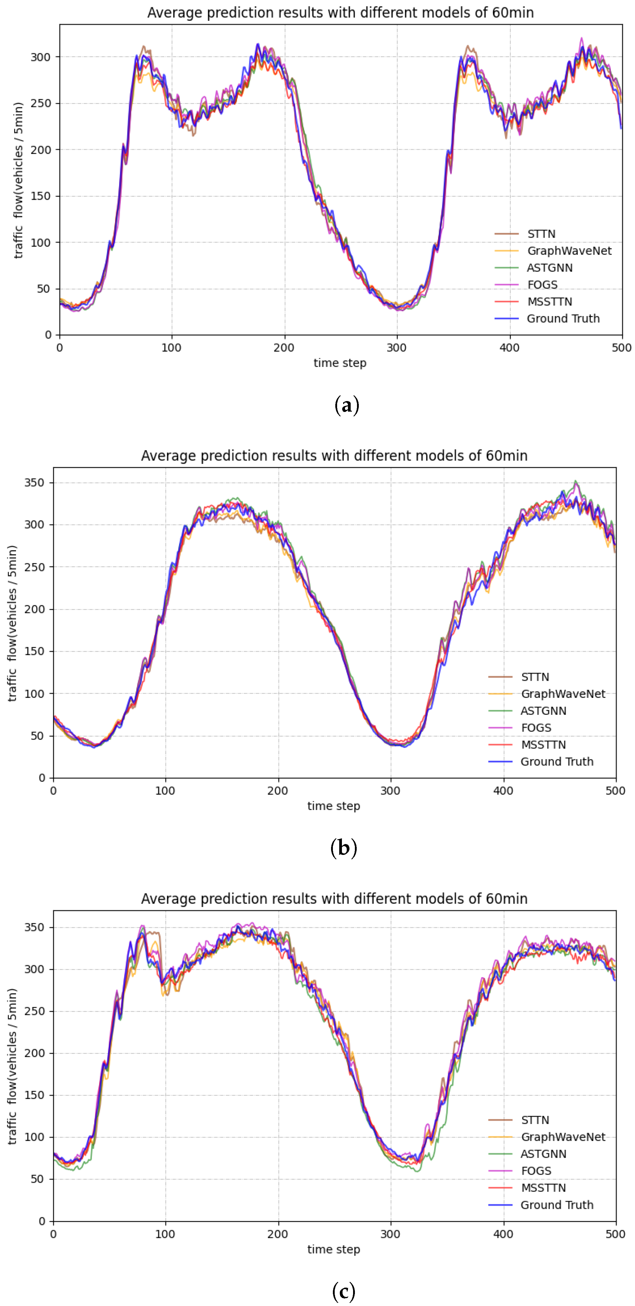Figure 7 shows the 60 min prediction results on three datasets as examples, and it is obvious that the prediction data made by MSSTTN is closest to the actual real-world data.

4.5. Ablation Experiments

This section presents a comprehensive analysis of the proposed MSSTTN model through extensive experiments conducted on the PEMS04 dataset. The aim is to verify the aforementioned improvement.

For the temporal aspect, we design two ablation versions of MSSTTN:

(1)

MSSTTN-attn. This model removes the improved autoformer and replaces it with a self-attention-based transformer structure.

(2)

MSSTTN-single-i. This model extracts the trend-cyclical part by a single scale i that removes the multi-scale series decomposition.

For the spatial aspect, we also design two ablation versions of MSSTTN:

(1)

MSSTTN-GCN. This model replaces the improved GWNN with a two-layer GCN.

(2)

MSSTTN-fixed. This model disables the scaling parameter learning so that the GWNN doesn’t learn adaptive weights on graph signals of multi-scale frequencies.

Table 6. Comparison of ablation models.

Model	MAE	MAPE (%)	RMSE
MSSTTN	18.64/18.97/19.44/20.05	13.16/13.41/13.69/14.29	30.17/30.81/31.54/32.39
MSSTTN-attn	19.93/21.21/22.45/23.91	14.17/15.03/15.89/17.02	31.17/33.06/34.80/36.70
MSSTTN-single-3	19.03/19.46/19.99/20.76	13.44/13.75/14.21/14.92	30.53/31.29/32.09/33.09
MSSTTN-single-5	18.70/19.06/19.49/20.07	13.22/13.53/13.89/14.46	30.21/30.87/31.56/32.36
MSSTTN-single-7	18.68/19.00/19.45/20.04	13.08/13.30/13.67/14.24	30.28/30.89/31.61/32.40
MSSTTN-GCN	18.69/19.02/19.46/20.11	13.05/13.30/13.67/14.40	30.42/31.04/31.76/32.63
MSSTTN-fixed	18.63/18.98/19.43/20.04	13.16/13.48/13.82/14.37	30.19/30.86/31.58/32.41

shows the MAE, MAPE, and RMSE of 3, 6, 9, and 12 (15, 30, 45, and 60 min) prediction results of MSSTTN and the ablation models. Every hyperparameter setting in the unablated modules are the same as described in Section 4.2. From Table 6, we can conclude that:

• From the spatial aspect, the MSSTTN-fixed outperforms the MSSTTN-GCN, demonstrating that for capturing the fixed spatial dependencies, the GWNN is naturally more appropriate than GCN, which aggregates the features inflexibly. Then, paying attention to the comparison of MSSTTN and MSSTTN-fixed, the overall performances of MSSTTN are all better. This validates that learning adaptive neighborhoods to enable graph signals passed in a multi-scale manner can improve the prediction precision.
• From the temporal aspect, MSSTTN-attn performs worst, verifying that the time series analysis and period-based operation can strengthen the temporal dependencies modeling, especially in the long-term. Comparing all the MSSTTN(single-i), we can observe that the appropriate long-term trend is more valuable than the short-term trend for capturing temporal dependencies. MSSTTN outperforms all the MSSTTN(single-i), demonstrating that each of the various scale trend-cyclical parts is helpful for time series analysis, so the multi-scale series decomposition we propose is an effective method. Through all the ablation experiments, we can easily understand the usefulness of all the improvements we have made.

4.6. Hyperparameter Analysis

We conduct a series of experiments on PEMS04 to analyze the impact of hyperparameter tuning. The investigated hyperparameters are the number of encoder and decoder layers of the temporal autoformer, the number of spatial–temporal blocks, and the learning rate decay.

Table 7. Hyperparameter tuning.

Hyperparameter	Setting	MAE/MAPE (%)/RMSE
Encoder layers	1	20.05/14.29/32.39
	2	20.13/14.25/32.53
Decoder layers	1	20.31/14.45/32.64
	2	20.05/14.29/32.39
	3	20.11/14.27/32.46
Blocks	1	23.12/15.64/36.08
	2	21.89/14.96/34.21
	3	20.05/14.29/32.39

exhibit the results. The hyperparameter settings are the same as depicted in Section 4.2 except for the investigated changes. We can see that the proposed model is not sensitive to the number of encoder and decoder layers of temporal autoformer and is relatively sensitive to the number of spatial–temporal blocks.

4.7. Comparison on Rush Hours

We compare the results on rush hours in PEMS04 of MSSTTN and the four state-of-the-art baselines in

Table 8. Comparison of PEMS04 prediction results on rush hours.

Model	MAE	MAPE (%)	RMSE
GraphWaveNet	24.18/25.45/28.04	9.30/9.86/10.71	36.21/38.15/41.30
STTNs	24.10/25.34/27.73	9.62/10.02/10.87	36.33/38.07/41.00
ASTGNN	23.98/25.64/28.21	9.38/10.04/11.14	36.21/38.43/41.61
FOGS	24.15/25.72/28.12	9.39/9.96/10.97	36.36/38.48/41.53
MSSTTN	24.28/24.77/26.02	9.65/9.85/10.35	36.67/37.52/39.16

. The rush hours are considered 8:00–20:00. It is obvious that MSSTTN performs relatively poorly on short-term prediction (15 min) but still outperforms the baselines on long-term prediction. This verifies that the robustness of MSSTTN is excellent.

5. Conclusions

This paper proposes a novel model for long-term spatial–temporal prediction called multi-scale spatial–temporal transformer network that is based on an improved STTNs. Introducing the GWNN and autoformer, MSSTTN models spatial–temporal dependencies in a multi-scale manner. We enable the scaling parameter to be learnable to pass the graph signals and construct a trend-cyclical part extraction method in a multi-scale manner to enhance the time series analysis. Otherwise, the series decomposition and Auto-Correlation mechanism in autoformer endow MSSTTN with powerful time series analysis ability. Based on series decomposition, this paper proposes a multi-scale decomposition method using windows of various scales to enhance the time series analysis ability. Experiments on three real-world datasets demonstrate that MSSTTN is superior in long-term spatial–temporal prediction.

Nevertheless, the complexity of autoformer gives MSSTTN a relatively high complexity, and graph wavelets must be recomputed during scaling the parameter learning. These result in certain computations. In future work, how to reduce the model complexity and simplify the recomputing of the graph wavelets while maintaining the prediction effect is a problem worth studying.