Principal Hugoniots of Promethium, Terbium, Thulium, Lutetium, and Actinium in a Wide Pressure Range

Abstract

We present the analytic forms of the principal Hugoniots of actinium (Ac) and the lanthanide promethium (Pm), which have both never been measured or calculated before, as well as those of terbium (Tb), thulium (Tm), and lutetium (Lu), the three least studied of the remaining lanthanides. They are based on our new analytic model of principal Hugoniot. A comparison of the five Hugoniots to our own independent theoretical calculations demonstrates very good agreement in every case, but each of the Hugoniots of Tb, Tm, and Ac from the TEFIS database, which ours are also compared to, appear to violate Johnson’s theoretical constraint $4<{\eta }_{\max }<7$ for the maximum compression ratio ${\eta }_{\max }$, which corresponds to the Hugoniot turnaround point. Possible reason for this behavior of the TEFIS Hugoniots is briefly discussed.

1. Introduction

Rare earth $4f$ elements, or lanthanides, play a key role in modern day technological applications, such as computer memories and permanent magnets. Similarly, $5f$ element actinides, being the backbone of nuclear fission technologies for the production of energy, also find applications in many non-power strategic fields, from space exploration to medical diagnostic and treatments. Specifically, the first member of the $5f$-series, actinium (Ac), is a potential therapeutic agent for cancer and infectious diseases [1,2]. Additionally, rare-earth superhydrides have recently been discovered to have near room temperature $T_c$ for superconductors above megabar pressures (1 Mbar = 100 GPa) [3,4,5]. As such, understanding and predicting the material behavior of lanthanides is crucial. This can be done using equation of state (EOS) information; however, both $4f$-electron lanthanides and $5f$-electron actinides present a unique challenge in performing first-principles based ab initio calculations due to their complex electronic and lattice structures. Therefore, experimental EOS measurements are indispensable in providing benchmark data to tightly constrain the ab initio calculations. Research efforts on Ac, as well as some lanthanides, have been hampered by the lack of supply and the high costs of current production methods, especially for Ac, and the radioactivity of promethium (Pm). In fact, Pm is the only radioactive element among the lanthanides, and the second radioactive element after technetium (Tc) that has stable neighboring elements. Thus, the EOS data on both Pm and Ac are scarce and virtually non-existent. Lutetium (Lu), in contrast, has been the subject of intense studies, mainly because it is the last element in the lanthanide series and has a completely filled $4f$ shell. However, even with the availability of several EOS studies [6], there is only one published study of the shock compression of Lu, by Al’tshuler et al. [7]. Similarly, there is only one published study of the shock compression of both terbium (Tb) and thulium (Tm), by Carter et al. [8].

The shock Hugoniot, both the principal and second-shock one, is a continuous curve which describes the locus of all possible thermodynamic states a substance can exist in behind a shock propagating through it. It is usually given as a projection onto a two-dimensional plane and is described in terms of two coordinates which can be chosen among particle velocity behind the shock front $\left(U_p\right),$ shock velocity $\left(U_s\right),$ pressure, internal energy $\left(E\right),$ temperature $\left(T\right),$ density $\left(\rho \right),$ and degree of compression ($\eta$) called “compression” for simplicity. Up to P of a few hundred GPa, the Hugoniot is known from experiments, and in the vast majority of cases is described by a linear relation $U_s=C+B{U}_p,$ between the two main variables, $U_s$ and $U_p,$ in terms of which all other relevant quantities can be expressed via the Rankine–Hugoniot (RH) relations (which represent the conservation of mass, momentum, and energy, respectively):

$$\eta \equiv \frac{\rho }{{\rho }_0}=\frac{U_s}{U_s-U_p},P=P_0+{\rho }_0{U}_s{U}_p,E-E_0=\frac{1}{2}(P+P_0)\left(\frac{1}{{\rho }_0}-\frac{1}{\rho }\right),$$

(1)

where the subscript 0 indicates the initial (unshocked) state. For the principal Hugoniot, $P_0=0.$

Over decades of research, shock Hugoniot measurements have been one of the most important sources of EOS data. The use of planar shock waves to determine the EOS of condensed materials to very high pressure $\left(P\right)$ began in 1955 with the classic papers of Walsh and Christian (1955) [9] and Bancroft et al. (1956) [10]. Walsh and Christian described the use of in-contact explosives to determine dynamic pressure-volume relations for metals and compared these to the then available static compression data. Bancroft et al. described the first polymorphic phase change discovered in a solid via shock waves, namely, iron. Two years later, Al’tshuler et al. (1958) [11] reported the first data for iron to P of several Mbar, essentially in excess of P in the center of the Earth. Since that time, the EOSs of virtually hundreds or even thousands of condensed materials have been studied, including elements, compounds, alloys, rocks and minerals, polymers, fluids, and porous media. These studies have employed both conventional and nuclear explosive sources, as well as impactors launched with a range of guns to speeds of order of 10 km/s. Recently, with the establishment of the NIF Gigabar platform at the Lawrence Livermore National Laboratory [12], pressures of order of 1 Gbar (${10}^5$ GPa, or 100 TPa), deep into the atomic pressure regime, have been routinely achieved in their experiments [13] (in this regime, P exceeds $P_a,$, the so-called atomic pressure required to significantly distort core electron orbitals and estimated as $P_a=E_{\mathrm{H}}/r_{\mathrm{Bohr}}^3=294$ Mbar, where $E_{\mathrm{H}}$ is the Hartree energy and $r_{\mathrm{Bohr}}$ is the Bohr radius).

The lanthanides series includes lanthanum (La) and the 14 following elements in which the $4f$-electron shell gets progressively filled. This shell is half-filled for europium (Eu) and fully filled for ytterbium (Yb), which is responsible for both of them being divalent, in contrast to the remaining lanthanides, which are all trivalent, similar to their transition metal counterparts, scandium (Sc) and yttrium (Y). Because the $4f$-electrons are localized deep in the lanthanide atoms (specifically, in their Xe-cores), they do not participate in metallic bonding [14], which is dominated by the $5p$, $5d$, and $6s$ valence electrons. The typical electron structure of a lanthanide atom is [Xe]$4f^{n}5d^{0}6s^2$ or [Xe]$4f^{n-1}5d^{1}6s^2.$

The dominance of the $spd$-valence electrons in the bonding is responsible for the lanthanides’ phase diagrams to vary slowly across the series so that their relations to one another is clearly seen [15]. The well established fact about the lanthanides is that, with increasing $P,$ virtually all of them undergo the same sequence of phase transformations from one hexagonal polytype to the next; it is characterized by the varying hexagonal layer stacking of the corresponding crystal structure: hexagonal close-packed (hcp, AB) →$\alpha$-Sm (9R, ABCBCACAB) → double-hcp (dhcp, ABAC) → face-centered cubic (fcc, ABC) → distorted fcc (dfcc) →… Evans et al. [16] showed that the dfcc phase of praseodymium (Pr) is $hR24,$ another hexagonal polytype with 24 atoms per unit cell, i.e., with a stacking of 24 ABC-layers. $hR24,$ along with two alternative crystal structures, namely, orthorhombic $oI16$, and $oS8,$ were identified as dfcc for other lanthanides. Recently, a possible extension of the above phase transition sequence to include post-dfcc phases was suggested in Ref. [17].

The actinides form a similar series, from Ac to lawrencium (Lr), in which the $5f$-electron shell gets progressively filled. In this respect, a comparison of the phase diagrams of the two series is useful and informative, but in contrast to the lanthanides, the structural systematics for the actinides, in terms of a sequence of phase transformations on increasing P, is much less obvious for the light actinides, but becomes more obvious for the heavier actinies, starting with americium (Am) [18]: dhcp → fcc →$\alpha$-U →… Note that, again, in contrast to the lanthanides, $\alpha$-U is not one of the hexagonal polytypes.

The principal Hugoniots of lanthanides have been experimentally investigated in several studies, e.g., refs. [7,19], but only a few substances at a time. The systematic study of the Hugoniots for the lanthanide series as a whole was carried out in Refs. [8,20]. Specifically, 13 lanthanides out of 15 were studied in [8] (in addition to Sc and Y), and 9 in [20] (in addition to Sc, Y, and hafnium (Hf)). Both sets of data are generally consistent with each other: the numerical values of the parameters of the least-square linear fits to the corresponding $U_s$-$U_p$ data agree to within ∼15%. Here, $U_p$ and $U_s$ are particle and shock velocities, respectively. The unique feature of both sets of data is that for each substance, except cerium (Ce), the adequate description of the data in the whole $U_p$ region of up to ∼3.6 km/s requires a two-segment fit; that is, the lower and upper portions of the data sets are described by two distinct linear segments such that the combined two-segment graph is continuous, but not smooth, as the slope of the second segment (∼1.2–1.6) is ∼1.5 times higher than that of the first one (∼0.8–1.0). In each case, the change of slope happens at a compression of ∼1.6; the corresponding transition P increases from ∼20 GPa for the light lanthande members to ∼40 GPa for the heavy ones [8]. Eu and Yb are two exceptions, for which the transition P is ∼10 GPa. Additionally, the Eu data show the existence of a two-wave structure in the shock front, indicating a significant volume change at the transition, whereas in most of other cases, the data indicate that the volume change associated with this transition is either zero or very small [8]. Such $U_s$-$U_p$ behavior is typical of a solid–solid phase transformation or melting. In any event, the $U_s$-$U_p$ slope being ∼50% higher indicates that the compressibility of the emerging phase is changing more rapidly (the value of the P-derivative of the bulk modulus is higher). Direct evidence of phase transitions and melting along the principle Hugoniot in several lanthanide members using in-situ laser shock diffraction at the Dynamic Compression Sector was recently presented in [21].

In this work, we derive the analytic forms of the principal Hugoniots of Ac and Pm, which have both never been measured or calculated before, as well as those of Tb, Tm, and Lu, the three least studied of the remaining lanthanides. Indeed, the existing Hugoniot data on each of these three substances can only be found in a single literature source, namely, Ref. [8] for both Tb and Tm and Ref. [7] for Lu.

2. Principal Hugoniot in a Wide Pressure Range

We will construct the analytic models of the principal Hugoniots of the five substances, namely, Pm, Tb, Tm, Lu, and Ac, using the analytic framework established in our previous publication [22]. In this framework, a wide P range is divided into three regimes and the Hugoniot is constructed in each of these regimes and then interpolated smoothly between them. These regimes are: (i) the low-P regime in which the Hugoniot is described by $U_s=C+B{U}_p,$ where the values of C and B come from the experiment; (ii) the intermediate-P regime (discussed in more detail below) where the Hugoniot is described by the Thomas–Fermi–Kalitkin (TFK) model [23,24] $U_s=c+b{U}_p+a{U}_p^2,$ with the values of $c,$b, and a determined virtually for all Zs (Z being the atomic number) [23,24,25]; and (iii) the high-P regime in which the Hugoniot is described by the Debye-Hückel-Johnson (DHJ) model [26,27,28]. The only assumption made was that the principal Hugoniot is goverened by some function $U_s=U_s\left(U_p\right)$ (which is linear at low P and quadratic at intermediate $P;$ its high-P form was established in [22]) and that this function is continuous and smooth (the first derivative $d{U}_s/d{U}_p$ is continuous) at all $U_p.$ Then, it follows from the RH relations [22] that $\eta ,$P, and E are all continuous and smooth as well. No other assumption, and no additional free parameter except the six mentioned above, $C,$$B,$$c,$$b,$$a,$ and $Z,$ are required for the construction of the analytic model of the principal Hugoniot. In order to match the next regime, the linear form of the low-P regime is modified into $U_s=C+B{U}_p+A{U}_p^2,$ where A is an additional 7th parameter which introduces a very small non-linearity and is obtained using the formula $A=a-{(B-b)}^2/\left(4(c-C)\right)$ [22]. Since $a=\mathcal{O}\left({10}^{-5}\mathrm{s}/\mathrm{km}\right)$ and $c-C=\mathcal{O}\left(1\mathrm{km}/\mathrm{s}\right)$ (see, e.g.,

Table 1. Numerical values of the parameters for the analytic model of the principal Hugoniot for Pm, Tb, Tm, Lu, and Ac.

	Z	${\mathit{\rho }}_0$	C	B	$\mathit{A}\times {10}^2$	c	b	$\mathit{a}\times {10}^5$	L	d	$\mathit{f}\times {10}^3$	${\mathit{U}}_{\mathit{p}}^{*}$	${\mathit{U}}_{\mathit{p}}^{\mathbf{max}}$	${\mathit{U}}_{\mathit{p}}^{**}$
Pm	61	7.25	1.68	1.34	−0.401859	3.48843	1.16798	7.20958	116803	16.8604	−12.0145	21.0258	219.968	1532.46
Tb	65	8.23	1.72	1.29	−0.198052	3.53354	1.16804	6.99278	126383	36.9251	−17.0929	29.7399	224.792	1574.89
Tm	69	9.32	1.90	1.19	−6.83647 $\times {10}^{-5}$	3.63814	1.16834	6.67959	136038	20.3201	−12.2217	160.493	233.381	1649.44
Lu	71	9.84	0.98	1.65	−2.15897	3.65839	1.16833	6.56206	140890	19.4395	−11.7463	11.1213	236.116	1679.54
Ac	89	10.05	1.535	1.225	−0.109446	2.49698	1.15830	6.17184	185075	6.05256	−5.71868	28.8450	201.141	1913.82

below), the value of A depends on $B-b.$ Typically, this difference is of the order of 0.1; hence, $A\sim {10}^{-2}$ s/km. However, if this difference is small, so is $A,$ but $U_p^{*}$ in Equation (1), which determines the low-P–med-P transition point, is large, thus pushing the upper boundary of the low-P regime closer to the turnaround point. This is, e.g., the case of thulium considered in what follows for which $U_p^{*}\approx 160.5$ km/s is $\sim 2/3$ of $U_p^{\max }\approx 233.4$ km/s at the turnaround point (see Table 1); typically, $U_p^{*}\sim 0.1U_p^{\max }.$

The names of the three P regimes of the principal Hugoniot may sound confusing and may not correspond to those adapted in high-pressure research in general and phase diagram and EOS studies in particular. Specifically, it is generally adopted that high-P corresponds to pressures in excess of ∼100 GPa. In our case, the low-P–med-P transition point corresponds to shock velocities of ∼10 km/s (see, e.g., Table 1); with ambient density of ∼1–10 g/cm${}^3$, corresponding to a pressure of ∼100–1000 GPa. Thus, our med-P regime is analogous to the more familiar high-P range of EOS studies. Our med-P–high-P transition point corresponds to $P\sim$1–10 Gbar (${10}^5$–${10}^6$ GPa).

3. Methods

3.1. New Analytic Model for Principal Hugoniot

Here is a brief summary of the new analytic model, as per Ref. [22]. The new model is based on the following representation of the shock velocity $U_s$ as a function of the particle velocity $U_p$ over the three $U_p$ intervals, which is continuous and smooth from one interval to the next:

$$\begin{array}{ccc}{U}_s& =C+B{U}_p+A{U}_p^2,& 0\le U_p\le U_p^{*}=\frac{2(c-C)}{B-b}\\ U_s& =c+b{U}_p+a{U}_p^2,& U_p^{*}\le U_p\le U_p^{**}=n{U}_p^{*}\\ U_s& =-\frac{d}{\left|f\right|}+\frac{4}{3}{U}_p+\frac{d{U}_p}{1+\left|f\right|U_p},& U_p\ge U_p^{**}\end{array}$$

(2)

where $\left|f\right|$ stands for the absolute value of $f.$

The corresponding expressions for P along the principal Hugoniot are:

$$\begin{array}{ccc}P& =\frac{4{\rho }_0{C}^2\eta (\eta -1)}{{\{\eta -B(\eta -1)+\sqrt{{[\eta -B(\eta -1)]}^2-4AC{(\eta -1)}^2}\}}^2},& 0\le U_p\le U_p^{*}\\ P& =\frac{4{\rho }_0{c}^2\eta (\eta -1)}{{\{\eta -b(\eta -1)+\sqrt{{[\eta -b(\eta -1)]}^2-4ac{(\eta -1)}^2}\}}^2},& U_p^{*}\le U_p\le U_p^{\max }=\sqrt{\frac{c}{a}}\\ P& =\frac{4{\rho }_0{c}^2\eta (\eta -1)}{{\{\eta -b(\eta -1)-\sqrt{{[\eta -b(\eta -1)]}^2-4ac{(\eta -1)}^2}\}}^2},& U_p^{\max }\le U_p\le U_p^{**}\\ P& =\frac{{\rho }_0}{{4\left|f\right|}^2}\frac{\eta }{\eta -1}{\left(\sqrt{12d\frac{\eta -1}{\eta -4}+1}\mp 1\right)}^2,& U_p\ge U_p^{**}\end{array}$$

(3)

which define pressure along the Hugoniot as a continuous and smooth function of compression ratio $\eta \equiv \rho /{\rho }_0,$ where $\rho$ is density and the subscript 0 indicates the initial (unshocked) state. In the last equation of (3), the “−” sign corresponds to $f>0$ and the “+” sign to $f<0.$ Whereas d is always positive, it appears that f is positive for about 2/3 of the periodic table and negative for the remaining 1/3. In particular, f is negative for the entire lanthanide series, as well as for the early actinides, including Ac. Therefore, in our study, we use this equation with the “+” sign. The numerical values of d and f are defined by the formulas [22]:

$$\begin{array}{cc}f& =\frac{a[(4-3b)\sqrt{\frac{c}{a}}n-3c(1+n^2)]}{3a[L+c\sqrt{\frac{c}{a}}n(1+n^2)]-c(4-3b)n^2},\\ d& =L{\left\{\frac{a[(4-3b)\sqrt{\frac{c}{a}}n-3c(1+n^2)]}{3a[L+c\sqrt{\frac{c}{a}}n(1+n^2)]-c(4-3b)n^2}\right\}}^2,\end{array}$$

(4)

with $n=U_p^{**}/U_p^{\max },$$U_p^{**}$ being the (only positive) solution of Equation (5) below. The functions of $Z,$ d, and f are shown, respectively, in Figure 1 and Figure 2, and are not presented in [22].

In Equations (2) and (3), $0\le U_p\le U_p^{*}$ corresponds to the low-P regime, and $U_p^{*}\le U_p\le U_p^{**}$ and $U_p\ge U_p^{**}$ to the med-P and high-P regimes, respectively. The value of $U_p^{**}$ is found from Equation [22]:

$${\left[c+\left(b-\frac{4}{3}\right)U_p^{**}+a{U}_p^{**2}\right]}^2=L\left(b-\frac{4}{3}+2a{U}_p^{**}\right),$$

(5)

where [22]:

$$L=\frac{875Z^{2.4}}{A}\approx \frac{875Z^{2.4}}{2Z+0.006Z^2}{\left(\frac{\mathrm{km}}{\mathrm{s}}\right)}^2,$$

(6)

where A is the atomic mass.

3.2. The Choice of the Five Sets of the Hugoniot Parameters

Whereas the parameters $c,$b, and a for the med-P regime are available for all substances, and, therefore, d and f for the high-P regime can be calculated for all substances from Equation (4) with $n=U_p^{**}/U_p^{\max },$ where $U_p^{\max }=\sqrt{c/a}$ and $U_p^{**}$ satisfies Equation (5), the parameters C and B for the low-P regime must be specified (and then $A=a-{(B-b)}^2/\left(4(c-C)\right)$ [22]). Here, we use the original version of the analytic Hugoniot model [22], which describes the entire low-P regime in terms of a single $(C,B,A)$ parameter set, regardless of whether the actual low-P portion of the Hugoniot is multi-segment (two or more linear segments forming a continuous broken line, just as for the lanthanides), or multi-linear (two or more quasi-parallel segments, which is the case of, e.g., zirconium [29]), or a combination of both. In our case of the four lanthanides, it is logical to describe the low-P regime in terms of the corresponding parameters of the upper segment of the two-segment portion in order to match the upper segment directly with the med-P regime. These values come from [8] for Tb and Tm, and from [7] for Lu. Since no $(C,B)$ data exist on Pm, we obtain both values from smooth interpolation of the corresponding values for other members across the entire lanthanide series based on the results of [8,20]. For Ac, for which no $(C,B)$ data exist either, assuming that it is a single-phase material (in fact, Ac is fcc, and there is no evidence for a phase transition to any other solid phase [18]), two parameters can be calculated as [26,27] $C=\sqrt{{\mathcal{B}}_s\left({\rho }_0\right)/{\rho }_0}$ and $B=({\mathcal{B}}_s^{\prime }\left({\rho }_0\right)+1)/4,$ with bulk modulus ${\mathcal{B}}_s\left({\rho }_0\right)$ and its P-derivative ${\mathcal{B}}_s^{\prime }\left({\rho }_0\right)$ coming from the corresponding EOS. The best fit to the ab initio data on the EOS of Ac of Ref. [30] of the third-order Birch–Murnaghan form results in ${\mathcal{B}}_s\left({\rho }_0\right)=23.7\pm 3.7$ GPa and ${\mathcal{B}}_s^{\prime }\left({\rho }_0\right)=3.9\pm 0.3;$ therefore, with ${\rho }_0=10.05$ g/cm${}^3,$$C=\sqrt{23.7/10.05}=1.535$ km/s, and $B=(3.9+1)/4=1.225.$ Table 1 contains all the five complete sets of the Hugoniot parameters.

4. Results

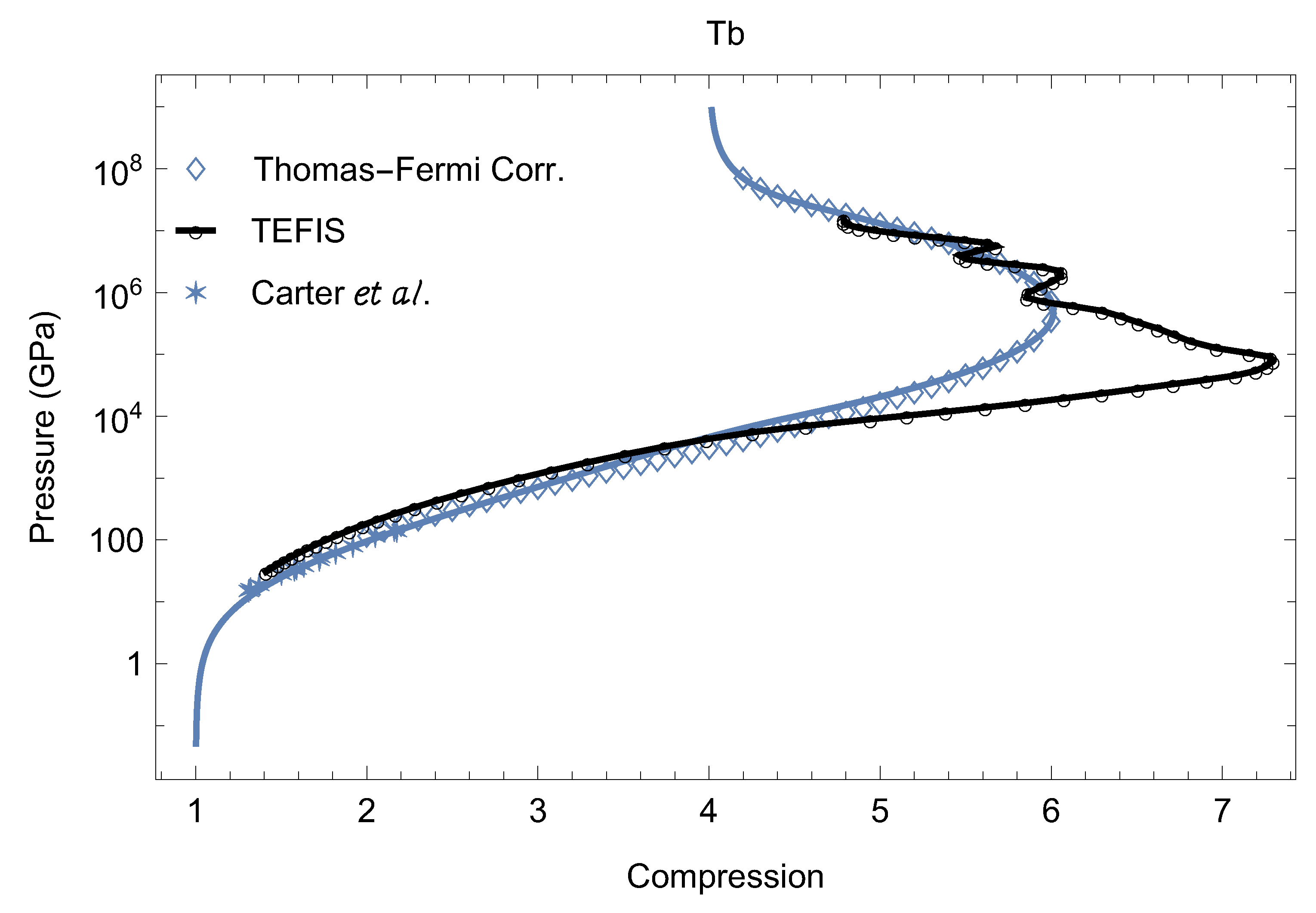
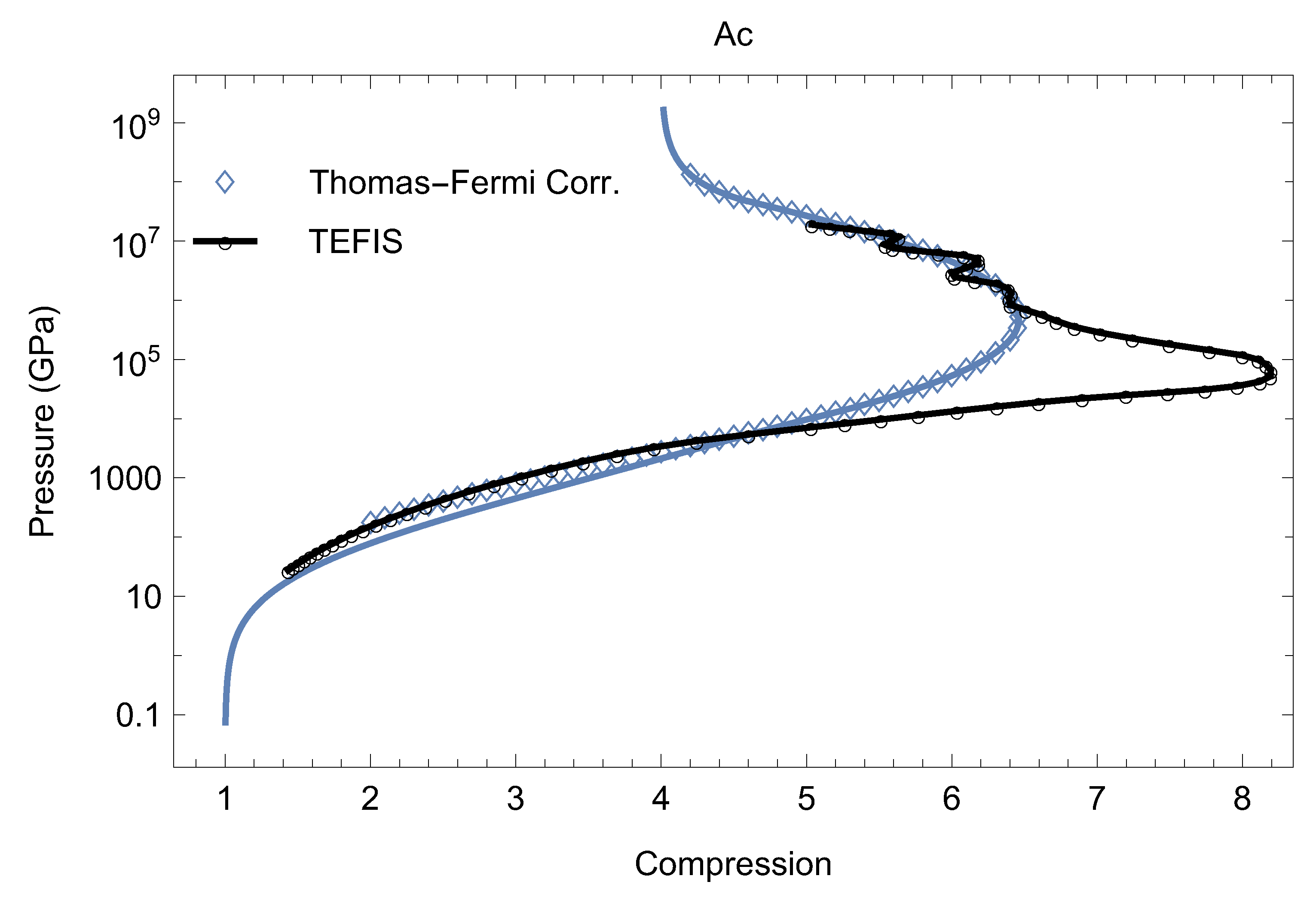
The five principal Hugoniots of the substances discussed in this work are shown in Figure 3, Figure 4, Figure 5, Figure 6 and Figure 7, in which the five Hugoniots are compared to both independent theoretical calculations and the available experimental data.

In addition to the available experimental data (for Tb, Tm, and Lu), for the purpose of comparison to the new analytic model, we have carried out theoretical Hugoniot calculations using: (i) the relativistic Green’s function quantum average atom code Tartarus [31,32] for Pm and Lu; and (ii) the Thomas–Fermi model with corrections [33] for Tb, Tm, and Ac, for which Lambert’s orbital-free molecular dynamics (OFMD) code used, e.g., in a study on the transport properties of lithium hydride [34], was modified appropriately. These simulations are similar to those of Ref. [35] for platinum. The $(V,P)$ points that map out the Hugoniot (presented in the $\eta$-P coordinates upon conversion of the $(V,P)$ points into the $(\eta ,P)$ ones) are found from the RH relation for internal energy: $E-E_0=P(V_0-V)/2.$ We also used three Hugoniots from the TEFIS database [36,37] for Tb, Tm, and Ac for the comparison to the new model, as well as to the Thomas–Fermi model with corrections. We note that, although Lu is an example of the application of Tartarus to a real material considered in detail in Ref. [32], the Lu Hugoniot shown in Figure 4 is not presented in [32].

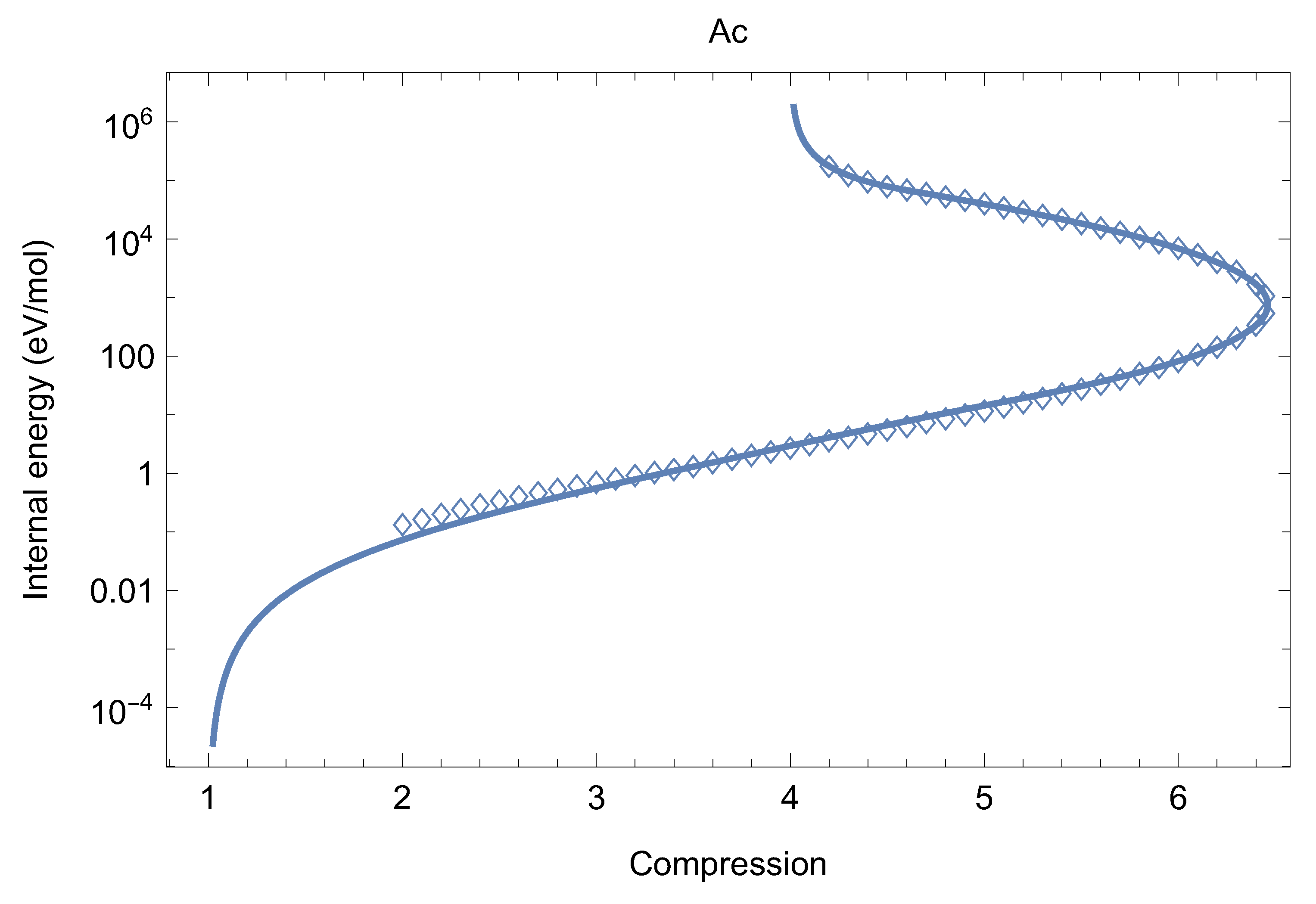
Similar to $P=P\left(\eta \right),$E along the Hugoniot can be calculated using the corresponding RH relation (1) for $E,$

$$E=E_0+\frac{P}{2{\rho }_0}\left(1-\frac{1}{\eta }\right),$$

(7)

and Equations (3) for $P=P\left(\eta \right)$ in the corresponding $U_p$ intervals. Figure 8 shows $E=E\left(\eta \right)$ for Ac (we assumed $E_0=0,$ for simplicity).

It is clearly seen that the forms of $P=P\left(\eta \right)$ and $E=E\left(\eta \right)$ are very similar to each other. The form of $T=T\left(\eta \right)$ is also expected to be similar to both $P=P\left(\eta \right)$ and $E=E\left(\eta \right).$ However, the accurate calculation of $T=T\left(\eta \right)$ requires the knowledge of the specific heat along the Hugoniot; hence, this calculation goes well beyond the scope of this work. We can, however, estimate the value of $T,$ based on that of $E,$ and compare it to the corresponding value from the TEFIS tables. For an ideal gas (which the system well above the turnaround point represents), $E\approx 3/2k_{B}T,$ at the upper limit of $E=E\left(\eta \right)$$k_{B}T\approx 2/3E.$ The uppermost TEFIS point in Figure 7 corresponds to $\eta \approx 5.04.$ At this $\eta ,$ the TEFIS table of $T=T\left(\eta \right)$ gives $T={10}^4$ eV (a table of $E=E\left(\eta \right)$ does not exist), and our value of E is $E(\eta =5.04)\approx 3.8\times {10}^4$ eV/mol; therefore, the above relation gives $T\approx 2.5\times {10}^4$ eV. Thus, our value of T is about 2.5 times larger than TEFIS’ one, which directly corresponds with the fact that our P is larger than TEFIS’ one by roughly the same amount, as can be clearly seen in Figure 7.

5. Discussion

As Figure 3, Figure 4, Figure 5, Figure 6 and Figure 7 clearly demonstrate, in each of the five cases, the agreement between the new analytic model and independent data is very good except for the three Hugoniots from the TEFIS database. As a matter of fact, the three TEFIS Hugoniots appear to violate Johnson’s constraint $4<{\eta }_{\max }<7$, which is based on rigorous theoretical grounds. (We have determined that this is the case for the vast majority of TEFIS Hugoniots for other substances.)

It is worthwhile to dwell on Johnson’s constraint in some more detail. In Ref. [38], Johnson derives the formula for the maximum compression on the princial Hugoniot:

$${\eta }_{\max }=\frac{4(1+7\mathcal{C})}{1+4\mathcal{C}},$$

(8)

where $\mathcal{C}\cong 0.011A{Z}^{4.2}/\left[{\rho }_0{(1+Z)}^4\right].$ As can be clearly seen in Figure 4 of [22], this ${\eta }_{\max }$ and the one given by the new analytic model are in very good agreement with each other, which lends further support to both formulations. Johnson’s constraint now follows directly from (8):

$${\eta }_{\max }=\frac{4+28\mathcal{C}}{1+4\mathcal{C}}<\frac{7+28\mathcal{C}}{1+4\mathcal{C}}=7,$$

(9)

and:

$${\eta }_{\max }=\frac{4+28\mathcal{C}}{1+4\mathcal{C}}>\frac{4+16\mathcal{C}}{1+4\mathcal{C}}=4.$$

(10)

We believe, the reason for this behavior of TEFIS Hugoniots is the way these Hugoniots are constructed; specifically, the scheme used in Refs. [39,40] for the interpolation between the portion of the Hugoniot below and across the turnaround point described by the TFK model, and that above the turnaround point, which incorporates electron shell effects, such shell effects are clearly seen in Figure 4, Figure 5, and Figure 7 for Tb, Tm, and Ac, respectively. In other words, the violation of Johnson’s theoretical constraint by the TEFIS Hugoniots may be the artifact of the interpolation scheme used for their construction. Otherwise, for P below and above the turnaround point, $1<\eta \stackrel{<}{\sim }4$ and $\sim 4.5<\eta \stackrel{<}{\sim }6,$ agreement between the TEFIS Hugoniots and both the new analytic model and the Thomas–Fermi model with corrections is generally good.

Let us note that in a more realistic case of a shock compression of a substance beyond the corresponding turnaround point, the Hugoniot must be modeled by taking into account the well-known effects of the contribution of both the equilibrium radiation of hot plasma and relativistic effects [41,42,43,44]. Indeed, at a turnaround point, $U_p\sim 200$–250 km/s (see Table 1), which constitutes $\stackrel{<}{\sim }0.1$% of the speed of light, and at the med-P–high-P transition point, $U_p\cong 1700\pm 200$ km/s, about 0.5% of the speed of light. Hence, as the system enters the high-P regime, relativistic effects are expected to start manifesting themselves and eventually to dominate the evolution of the system at even higher $U_p.$ Our model can, in principle, be modified to incorporate these effects. For instance, taking into account the radiation-dominated (or the so-called strong shock) regime can be done by replacing equations for $U_s\left(U_p\right)$ and $P\left(\eta \right)$ describing the high-P regime with their counterparts stemming from the physics of a photon gas. This goes beyond the scope of the present work, but will be undertaken in one of our subsequent studies.

The new model discussed in this work does not incorporate potential electronic shell effects in the high-P regime. If present, they manifest themselves in terms of some “irregularities”, that is, changes of the sign of $dP/d\eta$ of the continuous line $P=P\left(\eta \right)$ over some (small) regions of $P;$ such “irregularities” are seen, e.g., in the Tartarus Hugoniots of both Pm and Lu around ${10}^5$–${10}^{6.5}$ GPa in Figure 3 and Figure 6, respectively, since Tartarus takes electronic shell effects into account explicitly. Similar irregularities are present in the TEFIS Hugoniots, but the corresponding changes of the sign of $dP/d\eta$ are very abrupt. This is because these Hugoniots are constructed the way that causes the violation of Johnson’s theoretical constraint, as discussed above. In contrast to Tartarus, the orbital-free procedure of the OFMD code treats all electrons on an equal footing, albeit approximately, with no distinction between bound and ionized electrons. This is why any shell-ionization related effects are absent in the corresponding Hugoniots, as seen in Figure 4, Figure 5, and Figure 7. Such effects cannot be predicted by the new model, but, if firmly established, they can be added to the model by considering additional region(s) of P described by the corresponding $U_s=U_s\left(U_p\right)$ functional forms. We plan to undertake such an addition of electronic shell effects to the new model in one of our subsequent studies on this subject.

6. Conclusions

Here is a brief summary of the findings of this work. We have presented the principal Hugoniots of actinium and the lanthanide promethium, which have both never been measured or calculated before, as well as those of terbium, thulium, and lutetium, the three least studied of the remaining lanthanides. We used the analytic framework established in our previous publication [22]. All five sets of the relevant parameters are summarized in Table 1. The five principal Hugoniots are compared to the available experimental data (for Tb and Tm only) and independent theoretical calculations in Figure 3, Figure 4, Figure 5, Figure 6 and Figure 7. As can be clearly seen in these figures, in each of the five cases, the agreement between the new analytic model and independent data is very good except for the three Hugoniots from the TEFIS database, which all violate Johnson’s theoretical constraint on the maximum compression. Their behavior is analyzed in some detail in our paper. We anticipate that new experimental measurements could shed more light on a potential systematics of the lanthanide Hugoniots in terms of the values of the parameters C and $B,$ the maximum compression ${\eta }_{\max },$ etc. We expect our results to serve as the initial guidance for such experiments.

Our new analytic model of the principal Hugoniot [22] can be used for the validation of the P-V-T EOS by comparing the Hugoniot produced by the EOS to that given by the model. Additionally, the new model itself can be used as a basis for EOS construction. Indeed, if the Grüneisen parameter along the Hugoniot is available, e.g., using the approach discussed in this work, then it can be used in the Mie-Grüneisen-type EOS $P-P_{\mathrm{H}}={\gamma }_{\mathrm{H}}\rho (E-E_{\mathrm{H}})$ [45], where the subscript “H” implies that the corresponding variable is in shock-compression conditions. This EOS can then be brought in direct correspondence to the more familiar Mie-Grüneisen (M-G) EOS, $P-P_c=\gamma \rho (E-E_c),$ where the subscript “c” implies the cold $(T=0)$ conditions, since there exists a direct algebraic connection between ${\gamma }_{\mathrm{H}}$ (of this work) and $\gamma$ of the M-G EOS [45].

The analytic model developed in our previous study [22] and applied to five substances in this work can be used to calculate of the Hugoniots of other substances, specifically, other lanthanides and/or actinides. In this respect, the analytic knowledge of the regimes of the Hugoniot past the turnaround point is very important. In a very recent publication [46], a team of astronomers report a detailed study of a pair of shock waves produced by a collision of two clusters of galaxies that occurred roughly a billion years ago. The shocks that are associated with cluster mergers are known as radio relics and they can be used to probe the properties of the intergalactic space within the cluster, known as the intracluster medium, as well as intracluster dynamics. The study focused on a particular cluster called Abell 3667, which at least 550 galaxies are associated with and which is still coming together. It was concluded that the shock waves are propagating through it at velocities of ∼1500 km/s, which are 5–6 times larger than the velocities corresponding to turnaround points [22], $U_s^{\max }=2c+b\sqrt{c/a}\approx b\sqrt{c/a}\sim 1.2U_p^{\max }\sim$250–300 km/s (see Table 1). Moreover, at such shock velocities, many elements, especially the low-Z ones, will be under the conditions that are beyond the validity of Kalitkin’s parabolic representation (5), i.e., in the high-P regime considered in this work. Hence, to predict the properties of the intracluster medium and to describe intracluster dynamics, an analytic model of the principal Hugoniot in the high-P regime is a must. Once the analytic formulas describing the high-P regime are available (the last lines of both systems of Equations (2) and (3)), the basic mechanical and thermodynamic properties of a material under intergalactic shock, such as the bulk modulus, the Grüneisen parameter, energy, temperature, etc., along the principal Hugoniot can be derived from the RH relations and Equation (16) using the new model and some additional assumptions on the Grüneisen $\gamma .$