Predicting the Surface Soil Texture of Cultivated Land via Hyperspectral Remote Sensing and Machine Learning: A Case Study in Jianghuai Hilly Area

Abstract

Soil reflectance spectra and hyperspectral images have great potential to monitor and evaluate soil texture in large-scale scenarios. In hilly areas, sand, clay, and silt have similar spectral characteristics in visible, near-infrared, and short-wave infrared (VNIR-SWIR) reflection spectra. Soil texture spectra belong to mixed spectra despite some differences in particle size, mineral composition, and water content, making their distinction difficult. The accurate identification of the content within different particle sizes is difficult as it involves capturing spectral reflection features. Therefore, this study aimed to predict soil texture content through machine learning and unmixing the soil texture’s spectra while also comparing their respective modelling performances. Taking typical cultivated land in the Jianghuai hills as an example, the GaoFen-5 Advanced Hyperspectral Imaging (GF-5 AHSI) laboratory spectra of soil samples were used to predict sand, silt, and clay particle contents using partial least squares regression (PLSR) and convolutional neural networks (CNNs). The entire spectra of VNIR-SWIR regions were smoothed, and the dimensions were reduced via principal component analysis (PCA). The prediction models of sand, silt, and clay particle content were constructed, and inversion maps were generated using AHSI. The results showed that the PCA-CNN model achieved a higher prediction precision than the PCA-PLSR in both ASD and GF-5 data. Clay content exhibited the highest predictive performance with a coefficient of determination (R²) of 0.948 and 0.908 and a root mean square error (RMSE) of 26.51 g/kg and 31.24 g/kg, respectively, which represented a 39.0% and 79.8% increase in R² and a 57% and 57.1% decrease in RMSE compared to that of the PCA-PLSR. This method indicates that the PCA-CNN model can effectively achieve nonlinear interactions between multiple spectral components and better model and fit spectral mixing processes; moreover, it provides an alternative method for investigating the spatial distribution of soil texture.

1. Introduction

Soil texture refers to the distribution of mineral particles in the soil, which come in different shapes and sizes, and is closely related to various soil functions and qualities, including ion exchange dynamics, soil aeration, fertiliser retention, water retention, and chemical characteristics. It controls the soil’s water holding capacity, permeability, solute movement, and aeration, and dominates the soil’s physical, chemical, biological, and hydrological processes, which are closely related to plant growth and soil erosion [1,2]. Using soil mineralogy and grain size, it is crucial to swiftly and affordably detect the properties of soil texture and their spatial distribution for smart agricultural management, ecosystem services, environmental sustainability, and food security [3].

For a long time, laboratory analysis methods have mostly been used for soil texture analysis. The test results are reliable, but they are expensive, methodologically time consuming, labor intensive, and inefficient. Additionally, they may cause harmful reagents to have an impact on the environment. For instance, since soil texture and electromagnetic radiation physical characteristics are strongly related, the stretching and bending of N-H, O-H, and C-H are the primary causes of the soil’s spectral reflectance absorption characteristics [4,5,6]. The characteristics of different particle compositions within soil texture are thus captured by soil reflectance data, including particle size distribution, scattering, and absorption properties. Notably, sand has a noticeable effect on light scattering, which results in increased reflectivity in the visible and near-infrared spectral ranges. The reflectivity within these spectral regions is lower in silt and clay, which exhibit a relatively lesser scattering effect but absorb a significant quantity of light energy [7]. Therefore, via the analysis of soil reflectance data, the content of particles with different particle sizes in the soil and their interactions with light can be inferred. By using VNIR-SWIR spectroscopy (0.4–2.5 m), the geographic distribution of soil texture can be predicted without causing harmful damage [8].

In recent years, some scholars have conducted extensive research on soil properties, revealing the relationship between soil texture and VNIR-SWIR reflectance spectra. For example, the absorption peak of sand is usually around 900 nm, the absorption peak of clay is usually between 1400 nm and 1700 nm, and the absorption peak of silt is around 1900 nm–2200 nm [9,10]. When the position and intensity of these absorption peaks are detected, different types of soil can be extracted. After extensive tests, VNIR-SWIR reflectance spectroscopy is considered an alternative method for quickly predicting soil texture, promoting the transition from laboratory spectra to hyperspectral remote sensing images. Compared to laboratory spectral data, hyperspectral satellite images such as Hyperion and PRISMA have a wide range of repeated observations and coverage, which makes the accurate prediction of the spatial distribution of soil texture on a large scale possible [11,12]. At the same time, GF5 AHSI data have high spatiotemporal resolutions (30 m), wide widths, and richer spectral channels (330 bands). These data have been widely reported in soil attribute recognition and can be used to quantitatively estimate soil texture composition [13].

However, regardless of laboratory spectra or hyperspectral satellite data, a large number of studies have shown that the reflection spectra of sand, clay, and silt exhibit a similar trend within the VNIR-SWIR range, with higher reflectivity in the visible region, gradually stabilizing in the near-infrared region and gradually decreasing in the infrared region [14]. Although there are some differences in particle size, mineral composition, and water content, they may still have similar spectral characteristics. This is because soil particle size and mineral composition have similar effects on the overall amplitude of the reflection spectrum. In hilly areas, the mineral composition of sand, clay, and silt usually includes quartz, feldspar, illite, montmorillonite, and other components and is rich in organic matter and water from crystallization [15,16]. At 900 nm, 1400 nm, and 1900 nm, absorption peaks may appear in different types of soil with similar positions and amplitudes. In addition, the slope, degree of soil weathering, and drainage performance in hilly areas can affect the spectra. The mixing interaction of these factors mask the differences between sand, clay, and silt, making it difficult to distinguish them in the spectra [17,18,19].

The mixing effects of the reflection spectra of sand, clay, and silt in hilly areas make it difficult for traditional, empirical, or semi-empirical models to quantitatively detect soil texture content via their sensitive feature bands or their combinations [20,21]. In recent years, machine learning models have been proven to have the ability to learn complex patterns and object features using a large number of training data for model training, which helps improve the accuracy of classification and recognition. These models have been widely used in the fields of soil organic matter, organic carbon, heavy metals, etc. [22,23,24]. However, the mixed spectral unmixing and the prediction of the content of sand, clay, and silt in hilly areas have rarely been reported. CNN is a kind of feedforward neural network machine learning model that utilizes convolution computation and depth structure [25]. It has strong feature learning abilities. Via multi-layer convolution and pooling operations, high-level abstract features can be extracted from the original spectral data. These features can represent the characteristics of different components in the spectra and help to distinguish different components in the mixed spectra [26,27,28]. At the same time, via the non-linear mapping ability and model generalization ability of the neural network, a complex spectral mixing relationship can be modelled to reduce the cross-correlation between the mixed spectra of different soil particles and improve the prediction precision of soil texture content [29,30].

In this study, the laboratory spectra of soil samples and hyperspectral satellite remote sensing images were utilized to explore the performance of VNIR-SWIR hyperspectral data in predicting the content of sand, silt, and clay in soil texture. The aims of this study are as follows: (1) to evaluate the performance of machine learning models in mixed spectral unmixing between sand, silt, and clay in soil texture; (2) to evaluate the performance of laboratory spectra and hyperspectral images in predicting the content of sand, silt, and clay; (3) to evaluate the performance of hyperspectral images in mapping the spatial distribution of soil texture composition [31].

2. Materials and Methods

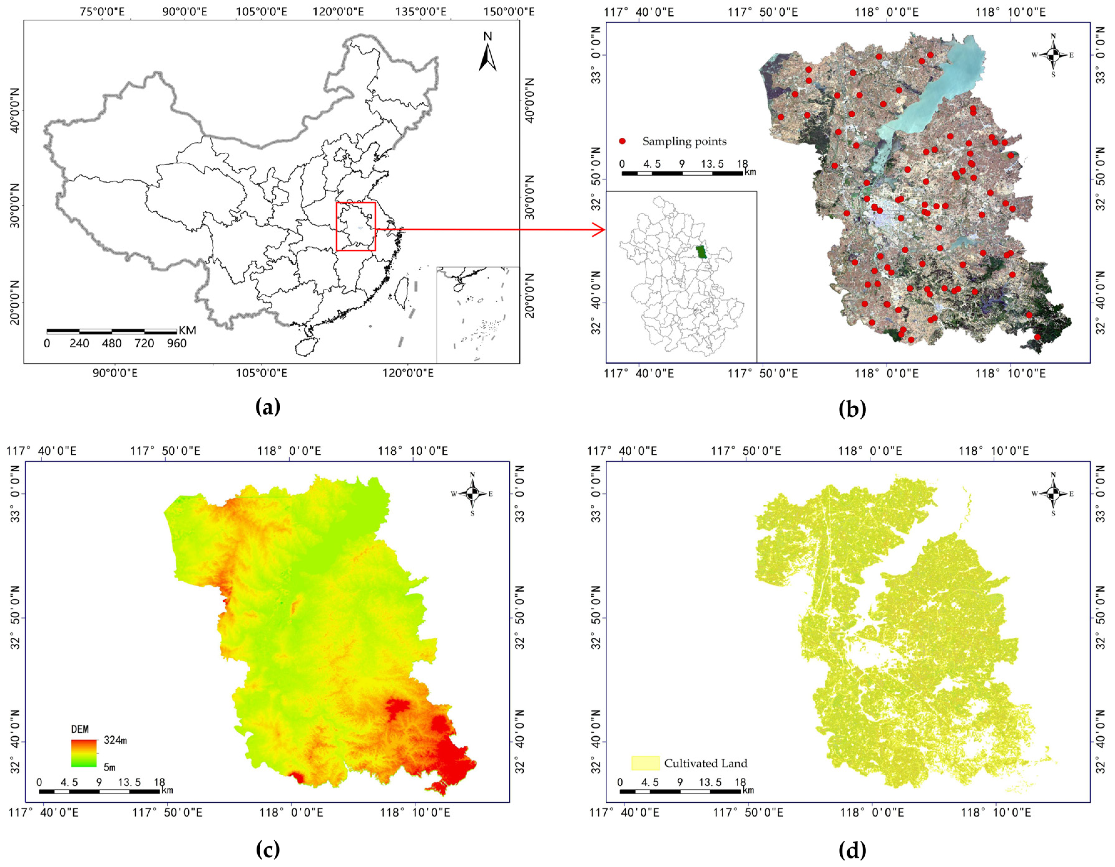
2.1. Study Area and Samples

The study area is located between 117.8° and 118.3° E and 32.5° and 33.1° N in the middle and western region of Mingguang County, Chuzhou City, Anhui Province. The South has high and the North has low terrain, with low mountains covering 35% of the total territory in the southern area, and the hilly region accounting for 47% of the total area in the middle and 10% of the plain area of the total area in the North. Additionally, lakes occupy 8% of the area, as shown in Figure 1a–c. The climate is characterized as a semi-humid monsoon with four distinct seasons with abundant sunshine, rain, and heat during one specific season with an average annual temperature of 15 °C and 934.1 mm of rainfall. It transitions from north subtropical to moderate temperate zones. Using a handheld GPS, 74 samples were placed simultaneously throughout the study area and uniformly collected under the location of the cultivated land at a sampling depth of 20 cm. The study region has a variety of soil textures, primarily clay loam, silty loam, silty clay, silty clay loam, loam, sandy loam, loamy sand, etc. [32].

The samples were examined following LY/T 1225-1999, the industry standard [33]. To determine the soil moisture conversion factor, air-dried soil samples of 50 g were measured through a 2 mm screen and then placed in a 500 mL conical flask. A dispersant was added in an amount determined by the pH of the soil. The mixture was then heated using a hot plate and then slightly cooled after boiling for 1 h. Later we separated the 2–0.25 μm particle size suspension using a 0.25 μm wash filter and funnel. For a grit of 0.25 to 2 mm, they were rinsed with water, dried, and placed in an aluminum box, and then the box was placed in an oven for 6 h before being weighed [34]. The suspension was stirred with a stirrer and placed in a densitometer after 30 s to record a 0.05 mm particle size reading. Another hydrometer reading for particles as small as 0.002 mm was collected after 8 h to produce soil samples of different particle sizes.

2.2. Data Acquisition

2.2.1. Data Acquisition of Soil Samples

The soil texture of the samples was classified by chemical testing methods according to the content of sand, silt and clay, with the highest and lowest content occurring in the sand grains, 816.9 g/kg and 9.1 g/kg, respectively, with a standard deviation of 170.7 g/kg, as shown in

Table 1. Statistical characteristics of the soil texture content.

Type	Max (g/kg)	Min (g/kg)	Mean (g/kg)	Standard Deviation (g/kg)
Sand particles	816.9	9.1	170.8	170.7
Silt	796.3	105.6	544.4	149.3
Clay	495.2	77.6	277.8	104.0
Total	816.9	9.1	331.0	213.1

.

2.2.2. Data Acquisition of GF5 AHSI

The GF5 HSI hyperspectral images were used with the acquisition date of 22 December 2019, which was synchronous with the sample collection date. The spatial resolution was 30 nm, the strip width was 60 km, and the spectral range was 390–2438 nm, with a total of 272 spectral bands, of which 143 bands were in the visible and near-infrared range (390–1000 nm), with a spectral resolution of 4.28 nm. 128 bands of short-wave infrared range (1000–2513 nm) had a spectral resolution of 8.42 nm. The sensor was affected by atmospheric water vapor absorption in the 1350–1400 nm and 1800–2000 nm bands, and the spectral data were discontinuous; therefore, 390–1317 nm, 1477–1739 nm, and 2007–2438 nm were chosen as the spectral ranges for this study. To eliminate the possible errors caused by atmospheric scattering and solar altitude angle on the spectral reflectance, ENVI 5.3 software was used to calibrate the image radiation and atmospheric correction. Then, ArcMap 10.6 software supplemented with GPS control point data was used to make fine geometric corrections to the image, and the corrected image was cropped according to the boundary of the study area to form the image of the regional basemap. Taking into account the influence of vegetation cover, different types of land, and the distribution of sample points on soil texture analysis, the 1:10,000 farmland status map was used to mask the processing and generate a thematic image map of the farmland area, as shown in Figure 1d.

2.2.3. Data Acquisition of Soil Sample Spectra

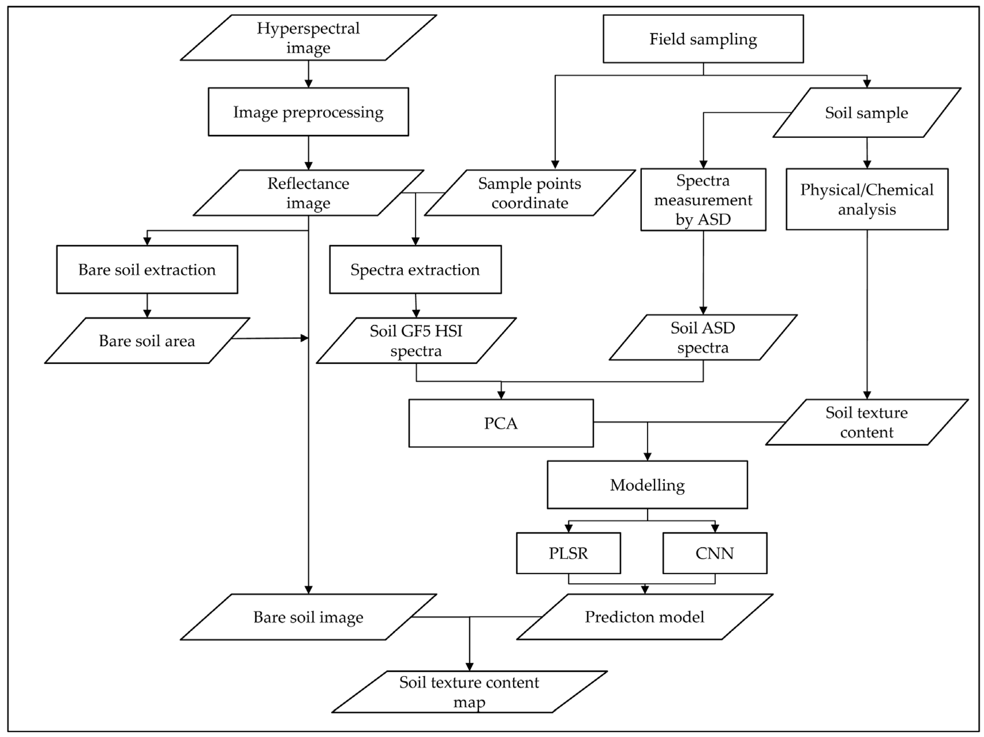
The hyperspectral reflectance of the acquired soil samples was measured in a dark room using a portable geophysical spectrometer, ASD FieldSpec Pro, with a 2000 W photographic spotlight as the light source at an illumination level of 39,800 lux/m and a spectral range of 350–2500 nm. The spectra were collected with the probe at a distance of 30 cm from the soil sample, with a field of view angle of 3° and vertical measurements [35]. The spectral sampling interval was 1.4 nm (350–1000 nm) and 2 nm (1000–2500 nm), and the resampling interval was set at 1 nm. Five spectral curves were acquired for each sample, and the average reflectance of the five measurements was used as the reflectance of the sample, and a total of 74 reflectance spectra were obtained for the samples in the spectral region of 350–2500 nm.

2.3. Methods

2.3.1. Principal Component Analysis (PCA)

PCA is a commonly used data dimensionality reduction for transforming high-dimensional data into low-dimensional data while retaining the primary information of the original data. It maps the original data into a new coordinate system through a linear transformation, such that the variance of the data is maximized under the new coordinate system. The specific steps are as follows:

(1)

Data normalisation: The original data is normalized to feature the mean value of 0 and a variance of 1 to eliminate the difference in magnitude between different features.

(2)

Calculate the covariance matrix: The covariance matrix describes the correlation between the different features.

(3)

Calculate the eigenvalues and eigenvectors: The covariance matrix is decomposed to obtain the eigenvalues and the corresponding eigenvectors. The eigenvalues represent the variance in the data in the direction of the eigenvectors, while the eigenvectors represent the projection direction of the data in the new coordinate system.

(4)

Selecting principal components: According to the magnitude of the eigenvalues, the eigenvectors correspond to the top k eigenvalues that are selected as principal components. The number of principal components k is usually selected based on the proportion of variance retained, and the calculation formula is the following:

$$F_k={\displaystyle \sum _{i=1}^k{\lambda }_i}/{\displaystyle \sum _{i=1}^{mk}{\lambda }_i}$$

(1)

(5)

Data transformation: The original data are projected onto the selected principal components to obtain the reduced-dimensionality data. The dimensionality of each sample in the new data set is reduced from the number of features in the original data to the number of selected principal components [36].

2.3.2. Modelling Methods

(1)

Partial Least Squares Regression (PLSR)

PLSR is a multivariate regression modelling method that can modify data in the presence of a strong correlation between variable components and solve the problem of complex data structures more effectively than standard classical regression analysis methods. The method combines the features of several regression analysis methods, including typical correlation analysis, multiple linear regression analysis, and principal component analysis, to provide a more comprehensive representation of information based on a suitable regression model [37]. In addition, the PLSR approach may also efficiently address the noise issue, minimize the spectral dimension, and emphasize the contributing reasons for variations in soil texture content [38].

(2)

Convolutional Neural Network (CNN)

CNN is a class of feedforward neural networks that includes convolutional computation, has a deep structure, and is one of the representative algorithms for deep learning. CNN has a powerful reinforcement feature capability, network parallel learning, and local weight sharing, reduces network complexity, and avoids the complexity of explicit feature extraction and data reconstruction, resulting in a higher-quality classification. CNN is well suited to the needs of soil monitoring and assessment since it can accurately and flexibly extract different soil properties from remote sensing images in spatial mode [25].

CNN is based on a hierarchical organization of neurons by learning to layer, with neurons between layers linked by deviations and weights. The network structure includes an initial layer, a middle layer, and an output layer. The initial layer is the input layer, which is used to input remote sensing data and sample point data. The middle layer is the hidden layer, which contains a convolutional layer, activation function, pooling layer, and fully connected layer, which is used to transform the output feature space and extract feature information. Finally, the output layer is used for predicted soil texture classification attributes [39].

The forward-propagation and backward-propagation phases comprise the two primary steps of the CNN training process. Forward-propagation feeds the input data into the network, and layer-by-layer propagation determines the output results. By determining the gradient of the loss function, backward-propagation adjusts the network parameters and brings the network output closer to the correct value [40].

The CNN model in this study was trained with an initial learning rate of 0.001 and an Adam optimizer. The network model used a minimum batch size of 30 and a maximum of epochs of 800. Dropout, early stopping, and reduction in the learning rate were used as a regularization technique, and to prevent overfitting of the network, the learning rate of the network model was set to be reduced to half of the initial learning rate at 400 epochs, and a dropout layer was added to the network model with a dropout rate of 0.30.

2.4. Model Evaluation

The model accuracy test is based on the standard regression and error-index evaluation, which reflects the degree of fit between the model modelling and the validation set and includes R², RMSE, and relative analytical error (RPD). The calculation formulae are, respectively:

$$R^2=\frac{{\displaystyle \sum _{i=1}^n{\widehat{y}}_i-{\overline{y}}^2}}{{\displaystyle \sum _{i=1}^n{y}_i-{\overline{y}}^2}}$$

(2)

$$RMSE=\sqrt{\frac{1}{n}{\displaystyle \sum _{i=1}^n{(y_i-{\widehat{y}}_i^{})}^2}}$$

(3)

$$RPD=\frac{SD}{RMSE}$$

(4)

where $\widehat{y_i}$ is the predicted soil texture, $y_i$ is the measured soil texture, $\overline{y}$ is the mean soil texture, n is the number of samples, and SD is the standard deviation [41].

R² determines the degree of explanation of the corresponding variable of the independent variable, ranging from 0 to 1, whereby the closer to 1, the better the model fits; RMSE measures the deviation between predicted and observed values, with a smaller RMSE indicating a smaller prediction error.

RPD is the ratio of the standard deviation of the sample SD to the standard error of the prediction, and RPD is used as a comprehensive measure of the predictive power of the model. The model is considered to have excellent quantitative predictive ability when RPD > 2, predicting the sample content when 1.4 < RPD < 2, and failing to predict the sample when RPD < 1.4.

2.5. Modelling

Forty-nine samples were selected as training samples, and twenty-five samples were selected as test samples, as shown in

Table 2. Descriptive statistics of the sample set.

Sample Set	Number	Type of Soil	Min (g/kg)	Max (g/kg)	Mean (g/kg)	Standard Deviation (g/kg)
Training Set	49	Sand	35.4	816.9	167.9	161.9
		Silt	105.6	796.3	556.72	134.92
		Clay	77.6	495.2	275.39	104.64
Validation Set	25	Sand	9.1	667.6	183.13	198.82
		Silt	191.6	770	528.02	151.99
		Clay	140.9	464.7	288.87	105.93

. The principal components of the PCA dimensionality reduction were used as independent variables (X), the ten principal components of the spectral data were used as model input variables, and the soil sample contents of different textures (sand, silt, and clay) were used as dependent variables (Y), and two dimensionality-reduced spectral datasets and soil sample contents of different textures were used to build the model using PCA-PLSR, and PCA-CNN algorithms were used to build remote sensing inversion models of soil texture, and the models were validated using test sample data. The stability and precision of the models were expressed by R² and RMSE. The PCA-PLSR and PCA-CNN modelling is implemented through MATLAB [16]. The flow chart for the prediction of soil texture content is shown in Figure 2.

3. Results

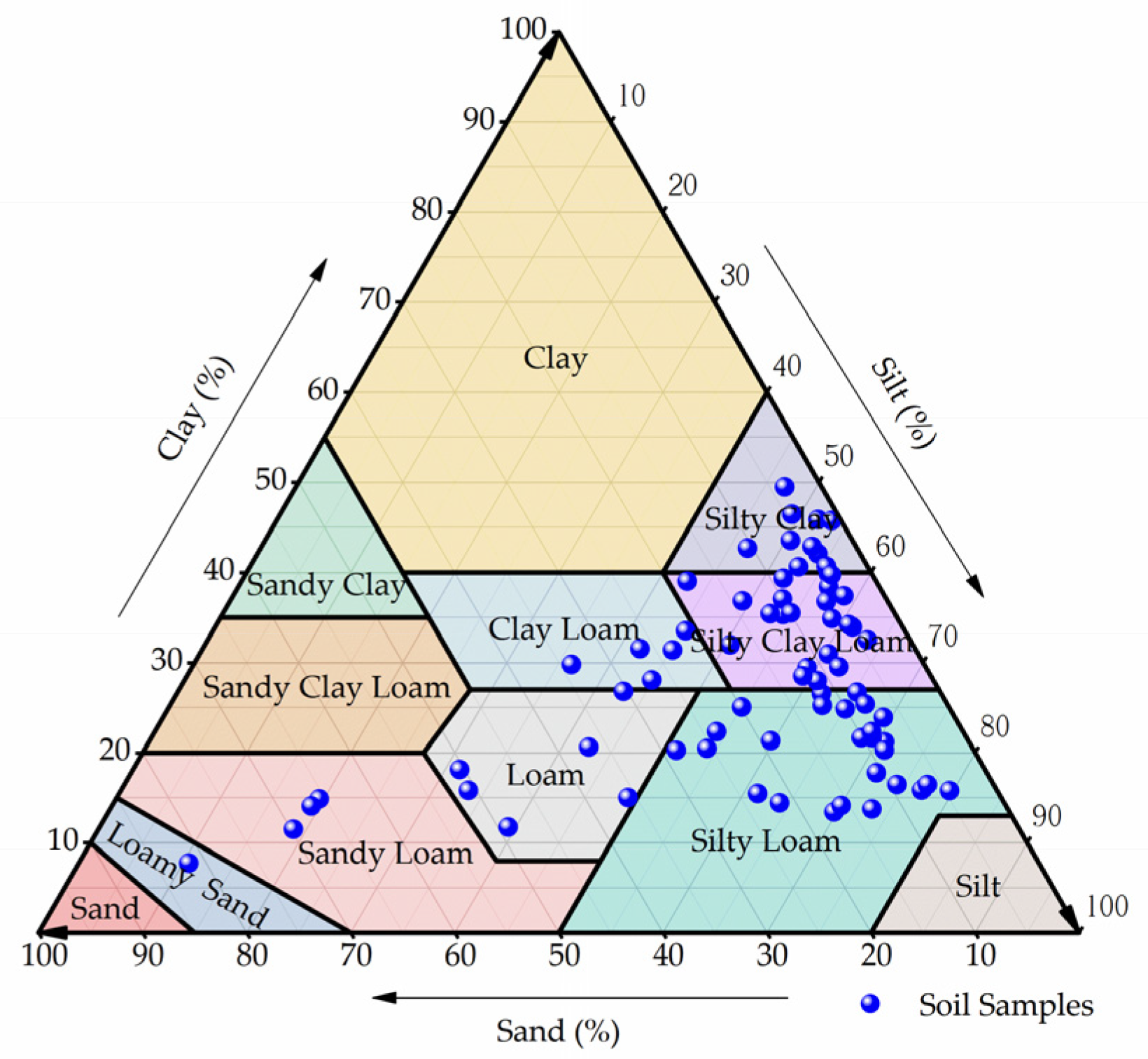
3.1. Description of Soil Properties

Based on the soil texture classification standard of the US system, the grain size of the samples was classified into clay (<0.002 mm), silt (0.002~0.05 mm), and sand (0.05~2 mm) according to the size of the soil, which was represented by a triangular coordinate diagram, as shown in Figure 3. The sides of the equilateral triangle represent the content of clay, flour, and sand grains, respectively (%) [42]. A soil texture consisting of 15% clay, 65% sand, and 20% meal is called sandy loam, while a soil texture consisting of 35% clay, 33% meal, and 32% sand is called clay loam. As can be seen from Figure 3, the soil texture types of the samples in the study area are mainly silty clay, silty clay loam, and silty loam, with a small proportion of soil types being loamy sand, sandy loam, and clay loam.

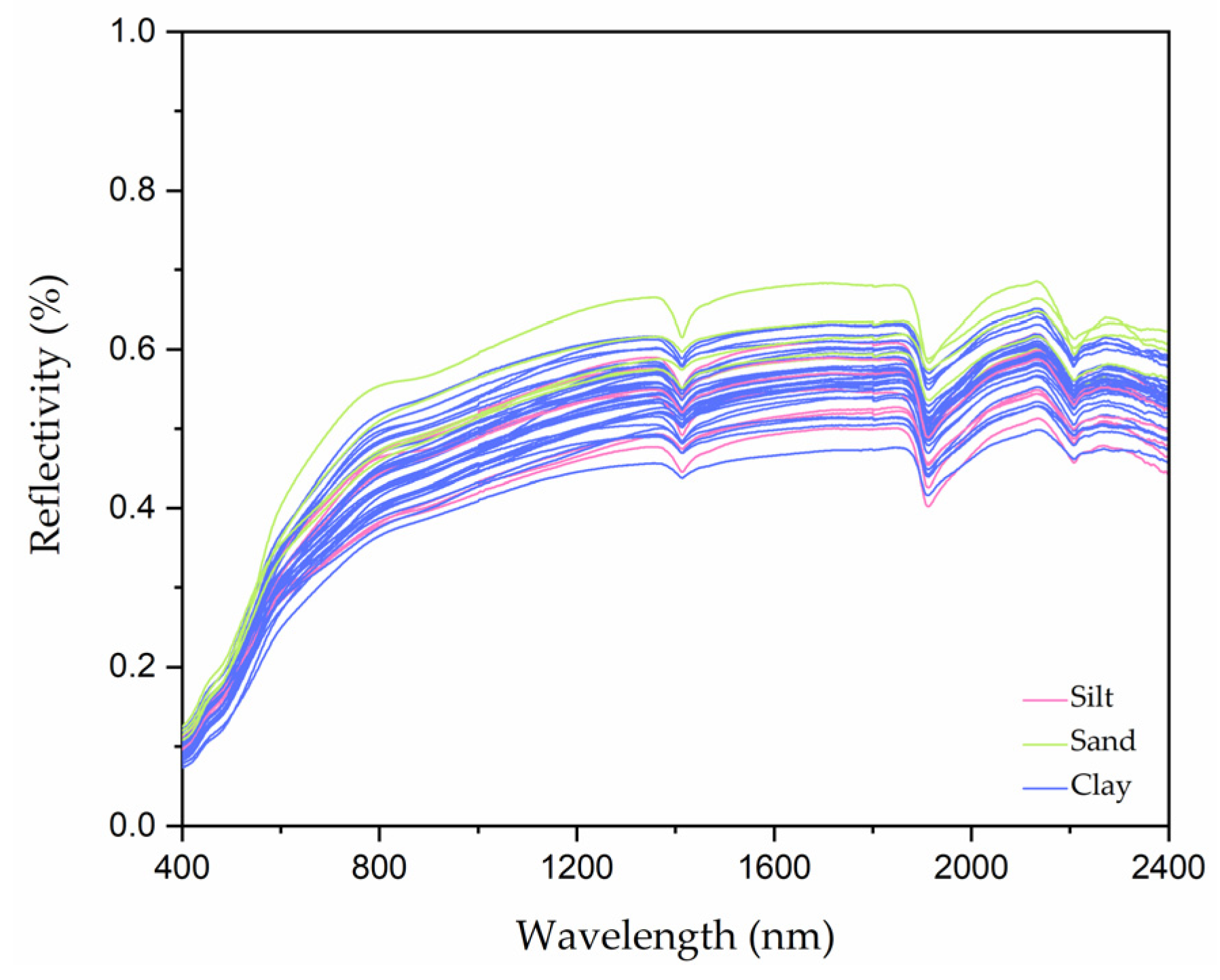
3.2. Spectral Characterisation

After the spectra were collected, the reflectance data were smoothed using the Savitzky–Golay method to prevent noise from interfering with the experimental results, as shown in Figure 4. The main characteristics are described in the following:

(1)

The surface-cultivated soil in the hilly regions has a high overall reflectance. Around 1400 nm, 1900 nm, and 2200 nm, there is an obvious water vapor absorption band, which is mainly caused by the vibration of water molecules in the soil [43].

(2)

From the reflection characteristics of sand, silt, and clay, the reflectivity increases with the increase in wavelength in the visible band, while in the near-infrared band, it has a higher reflectivity and tends to stabilize, with a reflectivity of up to 60%. After 2200 nm in the short-wave infrared band, the reflectivity shows a downward trend. The reflectance characteristics of three different types of soil particles are very similar. In hilly areas, the spectral mixing degree of clay and silt rich in illite and montmorillonite is higher, while the reflectance of sand rich in quartz and feldspar is slightly higher with a higher mixing degree with silt and clay [26].

3.3. Spectral Dimensionality Reduction

PCA is a commonly used method that reduces the dimensionality of linear data via linear variation to achieve the extraction of the original data. It supports a small number of unrelated variables (principal components) to describe the data and retains as much useful information as possible [36]. The PCA algorithm is used to reduce the dimension of the 330 bands of the ASD spectral data and the GF5 AHSI spectral data of the sample. To facilitate the subsequent image inversion of the sample area, the number of principal components of the spectral data from two different sources is taken as 10.

Table 3. Principal component contribution table.

Source of Data	ASD		GF5 HSI
Indicators	Contribution Rate/%	Cumulative Contribution Rate/%	Contribution Rate/%	Cumulative Contribution Rate/%
1	90.87	90.87	69.97	69.97
2	4.51	95.38	17.79	87.76
3	3.52	98.9	7.43	95.19
4	0.42	99.32	2.54	97.73
5	0.34	99.66	1.09	98.83
6	0.17	99.83	0.35	99.18
7	0.06	99.89	0.24	99.42
8	0.04	99.92	0.18	99.6
9	0.02	99.94	0.09	99.69
10	0.01	99.95	0.07	99.75

shows the contribution and cumulative contribution of the spectral principal components after dimensionality reduction.

3.4. Comparative Analysis of Modeling Results

Through the model validation, the effect of different characteristic variables on the prediction of the PLSR and CNN model after PCA screening were analyzed to select the best model for soil texture [44]. The model validation results are shown in

Table 4. Analysis of model validation accuracy.

Models	Particle Size	ASD			GF5 AHSI
		R2	RMSE (g/kg)	RPD	R2	RMSE (g/kg)	RPD
PCA-PLSR	Sand	0.644	112.23	1.23	0.573	124.85	1.28
	Silt	0.656	86.51	1.65	0.557	99.67	1.24
	Clay	0.682	61.65	1.64	0.505	72.75	1.13
PCA-CNN	Sand	0.853	81.55	1.65	0.857	72.46	2.23
	Silt	0.816	69.77	1.51	0.837	64.43	1.82
	Clay	0.948	26.51	3.33	0.908	31.24	3.13

.

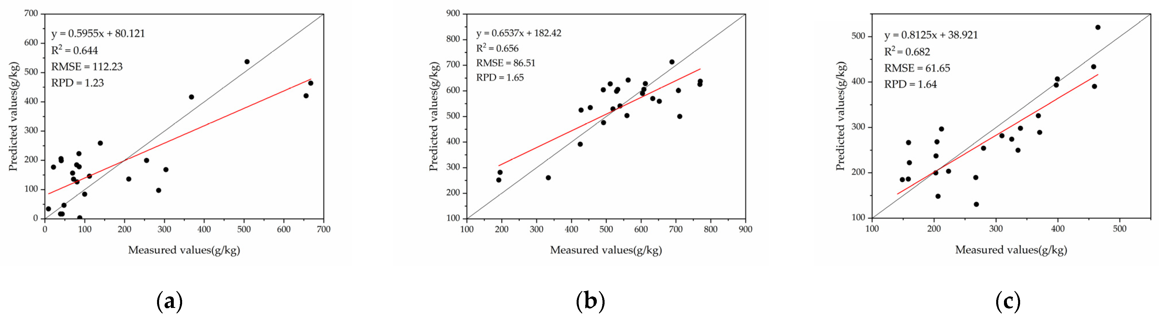
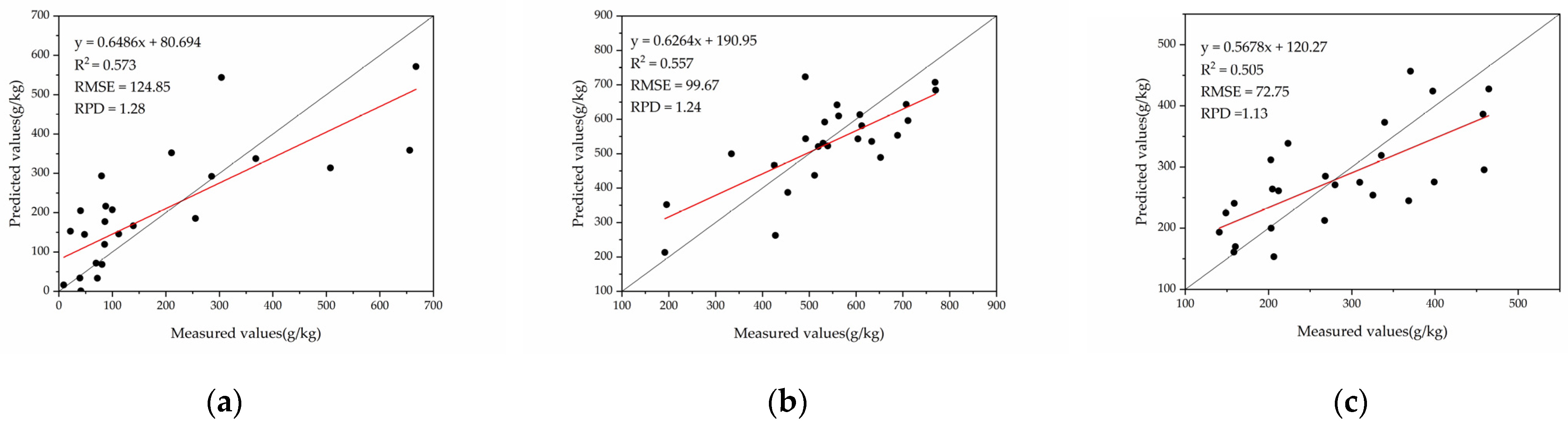
3.4.1. PCA-PLSR Modelling Results Analysis

As shown in Table 4 and in Figure 5 and Figure 6, the PCA-PLSR model using ASD spectral data and GF5 AHSI hyperspectral images have a certain predictive ability with R² in the range 0.50–50.682, RMSE in the range 61.65–124.85 g/kg, and RPD in the range 1.13–1.65. Among them, the predicted values of R², RMSE, and RPD using ASD spectral data are slightly better than those of GF5 AHSI hyperspectral images. Compared to laboratory data, hyperspectral data have a relatively low signal-to-noise ratio and are susceptible to limitations such as atmospheric attenuation, sensor radiation, and soil background environment.

In terms of sand, silt, and clay content, the prediction values of clay using ASD and GF5 AHSI data are higher than those of sand or silt, with an R² of 0.682, RMSE of 61.65 g/kg, and RPD of 1.64 for ASD, and an R² of 0.505, RMSE of 72.75 g/kg, and RPD of 1.13 for GF5 AHSI, reflecting that low-reflection clay is better predicted under controlled laboratory. Clay often has a strong water absorption ability, and its moisture content has a significant impact on its spectral characteristics, which can provide additional spectral information that helps to improve prediction accuracy. For sand and silt, their moisture content has a relatively small impact on spectral characteristics [45].

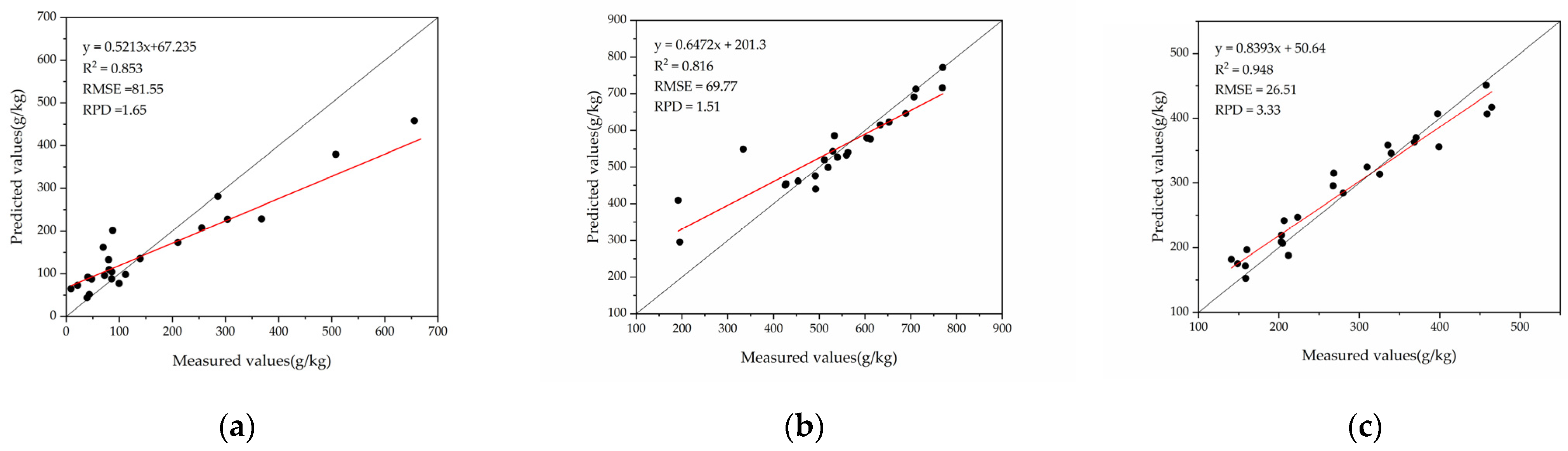
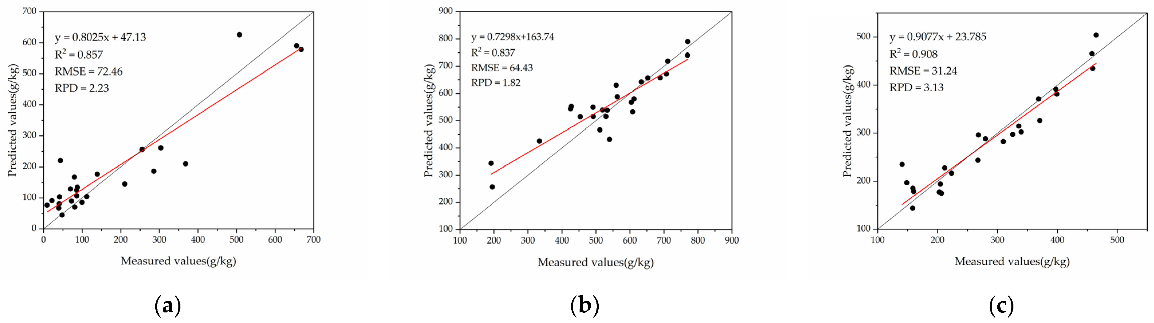
3.4.2. PCA-CNN Modeling Results Analysis

In Table 4, Figure 7 and Figure 8, the results of the PCA-CNN model using the ASD spectra data show R² is above 0.8, RMSE in the range 26.51–81.55 g/kg and RPD in the range 1.51–3.33, and the values of R² and RMSE are slightly higher than those of GF5 AHSI hyperspectral images. In terms of sand, silt, and clay content, the prediction values of clay using ASD and GF5 AHSI data are also higher than those of sand or silt, with ASD having a predicted value of R² of 0.948, RMSE of 26.51 g/kg, and RPD of 3.33 for clay and GF5 AHSI having a predicted value of R² of 0.908, RMSE of 31.24 g/kg, and RPD of 3.13 for clay, which are similar to the results of the PCA-PLSR algorithm. The high viscosity and plasticity of clay make it easier for PCA-CNN to capture and predict its properties, while its fine particles help algorithms analyze and model more accurately. The low-performance prediction of silt may be due to its ability to mix with sand and clay, with higher spectral mixing, making it more difficult to distinguish in the VNIR-SWIR region.

From the results of the ASD and GF5 AHSI data, the overall predicted precision of the GF5 AHSI data inversion is similar to that of the laboratory data. However, for sand and silt with higher reflectivity, the prediction results of GF5 AHSI data are higher than those of laboratory data, while for clay with lower reflectivity, the opposite is true. Compared to clay, the higher reflectivity of sand and silt exhibits strong contrast or tendency in remote sensing images. This makes it easier to be recognized by the PCA-CNN algorithm of images with a high classification accuracy. At the same time, for the soil texture of large particles, remote sensing images can better capture scale features, such as small slopes, surface texture, etc., providing more information and details in the recognition and classification process, which is conducive to improving the prediction accuracy [46].

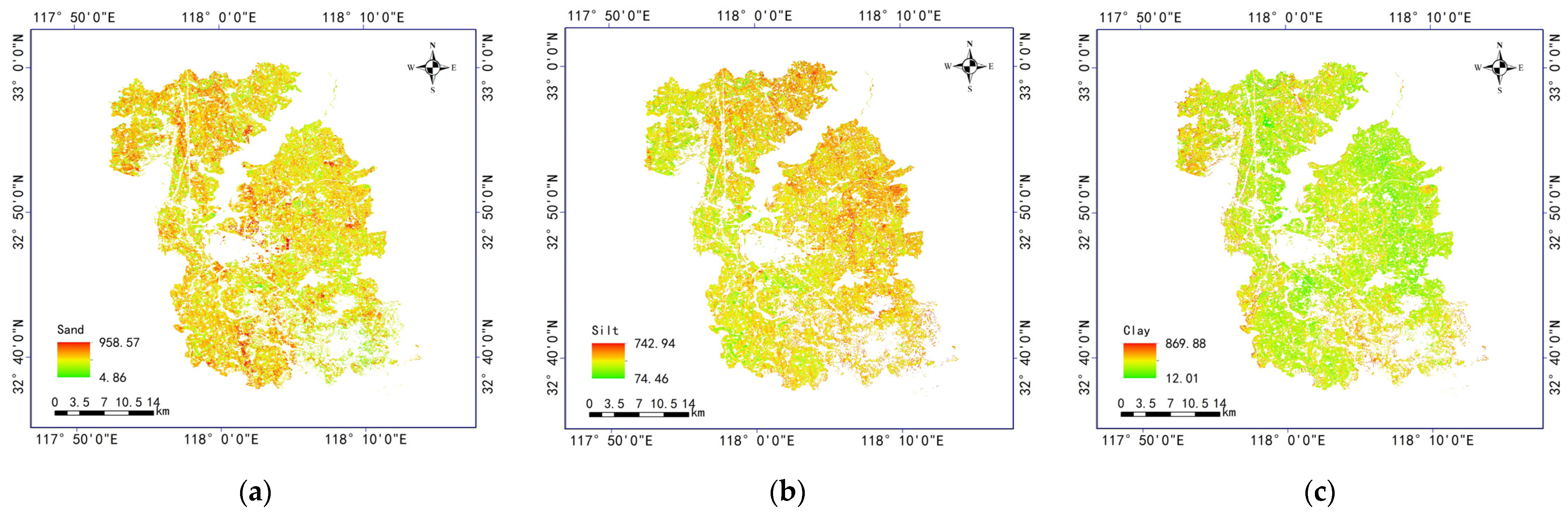
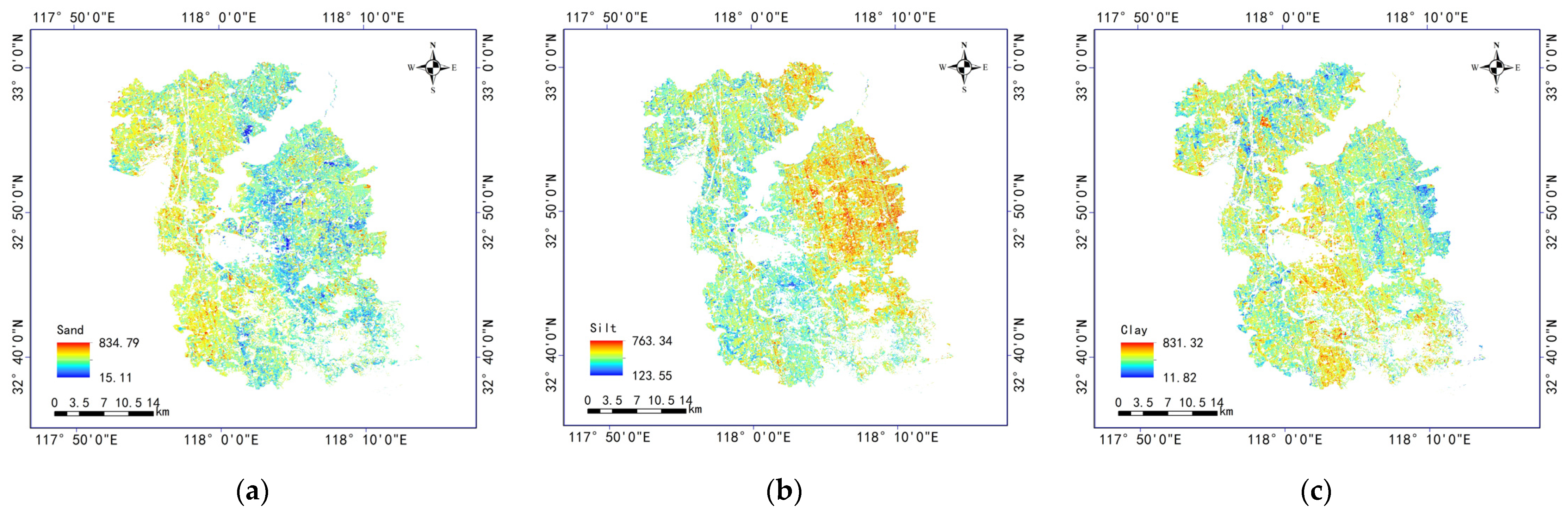
3.5. Model Inversion

By inputting the pre-processed remote sensing images into the trained PCA-CNN model for prediction, the distribution map of soil texture content estimation in the study area can be obtained, and the results are shown in Table 5 and in Figure 9 and Figure 10.

The map that predicts the texture of surface soil shows a similar distribution trend as that obtained by using the ASD spectra and GF5 AHSI hyperspectral data model. The study area on the western side has a high sand content compared to the eastern side. The southeastern uphill side of the study area has a low content of sand. However, the sand content is lower in the more upland areas on the southeastern side of the study area. The sand content is higher in the valleys with more sloping areas on the northwestern side of the study area. These sandy deposits have accumulated during natural erosion, causing them to deposit in the lowlands. The distribution of the silt content is the opposite of the sand content distribution, with the eastern side being higher than the western side; the area of the clay content distribution is relatively small, and the high values are mainly distributed in the southern and scattered areas in the north.

In terms of the inverse soil texture content, the range of content predicted by the ASD spectra is larger than that of the GF5 AHSI hyperspectral data, indicating that the ASD spectral predictions provide more information on the fine spatial distribution than the GF5 AHSI hyperspectral data.

Table 5. Statistics of the model inversion results based on the PCA-CNN algorithm.

Source of Data	ASD			GF5 AHSI
Type of Soil	Sand	Silt	Clay	Sand	Silt	Clay
Min (g/kg)	4.86	74.46	12.01	15.11	123.55	11.82
Max (g/kg)	958.57	742.94	869.88	834.79	763.34	831.32
Mean (g/kg)	470.79	577.02	239.28	121.42	542.49	327.83
Range (g/kg)	953.71	668.48	857.87	819.68	639.79	819.50

Table 5. Statistics of the model inversion results based on the PCA-CNN algorithm.

Source of Data	ASD			GF5 AHSI
Type of Soil	Sand	Silt	Clay	Sand	Silt	Clay
Min (g/kg)	4.86	74.46	12.01	15.11	123.55	11.82
Max (g/kg)	958.57	742.94	869.88	834.79	763.34	831.32
Mean (g/kg)	470.79	577.02	239.28	121.42	542.49	327.83
Range (g/kg)	953.71	668.48	857.87	819.68	639.79	819.50

4. Discussion

Among the two models mentioned above, the PCA-CNN model has better prediction results for the sand, silt, and clay content in soil texture inversion than the PCA-PLSR model as a whole. The PCA-CNN prediction model for sand, silt, and clay content based on the ASD spectral data was 32.5%, 24.4%, and 39.0% higher than the R² of PCA-PLSR, and the RMSE decreased by 27.3%, 19.4%, and 57.0%, respectively. And the RPD of all three PCA-CNN models is above 1.5. For the GF5 AHSI data, the R² of the PCA-CNN model was 49.6%, 50.3%, and 79.8% higher than that of the PCA-PLSR, the RMSE decreased by 42.0%, 35.4%, and 57.1%, and the RPD increased by 74.2%, 46.8%, and 177.0%, respectively. This is consistent with the results of Wartini Ng et al. and Lanfa Liu et al., who used a machine learning model based on VIS-NIR-SWIR spectroscopy to predict soil texture content and also obtained good prediction results [26,30]. Compared with the results of Reza Mirzaeitalarposti et al., they used three algorithms, including random forest (RF), support vector machine (SVM), and extreme gradient progression (XGB) to estimate the content of soil texture and predict that the R² of the optimal model reached 0.79, indicating that PCA-CNN has better non-linear unmixing and prediction capabilities than traditional machine learning [15].

Compared with PCA-PLSR, PCA-CNN has significant advantages in spectral unmixing and model prediction. It can automatically extract spatial and spectral features from spectral data through convolution and pooling layers. This allows the model to better capture the complex relationships between spectral data and the content of sand, silt, and clay. Because of its ability to capture local perception, non-linear modelling, and global information capture, CNN can more accurately perform spectral unmixing and simulate the non-linear relationship of complex spectra. At the same time, introducing PCA can effectively reduce feature dimensions, weaken computational complexity, and prevent overfitting that enables PCA-CNN to construct the model more accurately for complex nonlinear relationships, and it is suitable for solving the spectral overlap and diversity problems of sand, silt, and clay [46]. In contrast, PCA-PLSR, as a traditional spectral unmixing method, is usually based on linear assumptions and has poor modeling performance for complex nonlinear relationships, although it has certain applications in spectral unmixing. Significant errors may occur when PLSR is used to deal with nonlinear relationships. In addition, PCA-PLSR has high requirements for data quality, feature selection, and model parameter selection, which may require multiple pre-processing and adjustments. When processing high-dimensional spectral data, the computational complexity is high, resulting in certain limitations of this algorithm [47]. Therefore, in predicting soil texture content, PCA-CNN can better solve the nonlinear fitting problem between various soil texture forms.

Due to the high dimensional and complex nature of both the ASD spectral data and the GF5 AHSI image, the PCA-CNN model also suffers from a certain degree of overfitting, especially for the larger particle size loam particles, showing a certain lack of fault tolerance, resulting in a slight decrease in the predictive ability of the model. This requires further optimization for the model to be applied in intelligent detection and dynamic monitoring of soil texture.

Currently, PCA-CNN has only been validated on a small number of samples from a limited number of areas due to the limited dataset available, which restricts its generalizability. It is a data-deficient model that needs to be further explored by incorporating more soil samples, especially in areas with varying soil conditions. Furthermore, this method is limited to bare soil, and more research is needed on the effects of some external factors, such as vegetation cover and soil moisture [48]. Although the results obtained from hyperspectral images are still incompatible with laboratory spectra, PCA-CNN provides an alternative approach to mapping soil texture content using laboratory spectra and hyperspectral data.

5. Conclusions

In this study, the Jianghuai hilly region is set as an example to predict the sand, silt, and clay content of soil texture in the surface layer of arable land using GF5 AHSI hyperspectral satellite images and laboratory spectra with machine learning models. By contrasting PCA-PLSR and PCA-CNN, the performance of hyperspectral data for soil texture content prediction was assessed. The following are the key conclusions:

In the Jianghuai hilly area, soil texture is mainly composed of clay and silt. Sand, clay, and silt have similar spectral characteristics in the VNIR-SWIR reflection region with strong water vapor absorption near 1400 nm, 1900 nm, and 2200 nm. The results found that the prediction accuracy of clay content in soil texture was higher than that of sand and silt by using GF5 AHSI images and ASD spectra in hilly areas.

Compared with PCA-PLSR, PCA-CNN has a 32.5%, 24.4%, and 39.0% higher prediction index R² for sand, silt, and clay particles in the surface soil texture of cultivated land in hilly areas, while RMSE has decreased by 27.3%, 19.4%, and 57.0%, respectively. PCA-CNN has a strong nonlinear approximation ability. When predicting the content of sand, silt, and clay particles, it can effectively extract the characteristics of the input data and avoid spectral auto-correlation between different components of soil texture through multiple convolution kernels in the convolution layer perform convolution operations on the input spectral principal component data, which can better solve the problem of spectral unmixing among multiple soil texture forms.

According to the results of the remote sensing inversion, the sand grains of surface soil texture in the study area are mainly distributed in the west, the silt grains are distributed in the east, and some clay grains are scattered in the south and north, which are consistent with the soil mechanical composition of the sampling points. This indicates that there is a higher potential for quantitative monitoring of soil texture features using hyperspectral satellite remote sensing.

In summary, the PCA-CNN model can provide a fast and efficient monitoring method for predicting the surface soil texture content of cultivated land in the Jianghuai hilly area, greatly reducing the cost and time of soil texture detection, and providing an intelligent method for a thorough and dynamic understanding of regional soil quality. In this study, the GF5 satellite is sensitive to environmental factors such as terrain, vegetation and atmosphere in the retrieval process, and PCA-CNN still has limitations such as data dependency, lack of physical mechanism, and interpretability of spectral unmixing algorithm in spectral unmixing. Therefore, the practicality of the model still needs be further verified in different regions and soil properties [49].

References

1. Duan, M.; Song, X.; Liu, X.; Cui, D.; Zhang, X. Mapping the soil types combining multi-temporal remote sensing data with texture features. Comput. Electron. Agric. 2022, 200, 107230. [Google Scholar] [CrossRef]
2. Liao, K.; Xu, S.; Wu, J.; Zhu, Q. Spatial estimation of surface soil texture using remote sensing data. Soil Sci. Plant Nutr. 2013, 59, 488–500. [Google Scholar] [CrossRef]
3. Yang, M.; Xu, D.; Chen, S.; Li, H.; Shi, Z. Evaluation of Machine Learning Approaches to Predict Soil Organic Matter and pH Using vis-NIR Spectra. Sensors 2019, 19, 263. [Google Scholar] [CrossRef] [PubMed]
4. Karray, E.; Elmannai, H.; Toumi, E.; Hedi Gharbia, M.; Meshoul, S.; Aichi, H.; Ben Rabah, Z. Evaluating the Potentials of PLSR and SVR Models for Soil Properties Prediction Using Field Imaging, Laboratory VNIR Spectroscopy and Their Combination. Comput. Model. Eng. Sci. 2023, 136, 1399–1425. [Google Scholar] [CrossRef]
5. Nanni, M.R.; Demattê, J.A.M.; Rodrigues, M.; Santos, G.L.A.A.D.; Reis, A.S.; Oliveira, K.M.D.; Cezar, E.; Furlanetto, R.H.; Crusiol, L.G.T.; Sun, L. Mapping Particle Size and Soil Organic Matter in Tropical Soil Based on Hyperspectral Imaging and Non-Imaging Sensors. Remote Sens. 2021, 13, 1782. [Google Scholar] [CrossRef]
6. Sayão, V.M.; Demattê, J.A.M. Soil texture and organic carbon mapping using surface temperature and reflectance spectra in Southeast Brazil. Geoderma Reg. 2018, 14, e00174. [Google Scholar] [CrossRef]
7. Silva-Sangoi, D.V.D.; Horst, T.Z.; Moura-Bueno, J.M.; Dalmolin, R.S.D.; Sebem, E.; Gebler, L.; da Silva Santos, M. Soil organic matter and clay predictions by laboratory spectroscopy: Data spatial correlation. Geoderma Reg. 2022, 28, e00486. [Google Scholar] [CrossRef]
8. Reis, A.S.; Rodrigues, M.; Alemparte Abrantes dos Santos, G.L.; Mayara de Oliveira, K.; Furlanetto, R.H.; Teixeira Crusiol, L.G.; Cezar, E.; Nanni, M.R. Detection of soil organic matter using hyperspectral imaging sensor combined with multivariate regression modeling procedures. Remote Sens. Appl. Soc. Environ. 2021, 22, 100492. [Google Scholar] [CrossRef]
9. Ferreira, A.C.D.S.; Ceddia, M.B.; Costa, E.M.; Pinheiro, É.F.M.; Nascimento, M.M.D.; Vasques, G.M. Use of Airborne Radar Images and Machine Learning Algorithms to Map Soil Clay, Silt, and Sand Contents in Remote Areas under the Amazon Rainforest. Remote Sens. 2022, 14, 5711. [Google Scholar] [CrossRef]
10. Carvalho, J.K.; Moura-Bueno, J.M.; Ramon, R.; Almeida, T.F.; Naibo, G.; Martins, A.P.; Santos, L.S.; Gianello, C.; Tiecher, T. Combining different pre-processing and multivariate methods for prediction of soil organic matter by near infrared spectroscopy (NIRS) in Southern Brazil. Geoderma Reg. 2022, 29, e00530. [Google Scholar] [CrossRef]
11. Mallah Nowkandeh, S.; Noroozi, A.A.; Homaee, M. Estimating soil organic matter content from Hyperion reflectance images using PLSR, PCR, MinR and SWR models in semi-arid regions of Iran. Environ. Dev. 2018, 25, 23–32. [Google Scholar] [CrossRef]
12. Ewing, J.; Oommen, T.; Jayakumar, P.; Alger, R. Utilizing Hyperspectral Remote Sensing for Soil Gradation. Remote Sens. 2020, 12, 3312. [Google Scholar] [CrossRef]
13. Yin, F.; Wu, M.; Liu, L.; Zhu, Y.; Feng, J.; Yin, D.; Yin, C.; Yin, C. Predicting the abundance of copper in soil using reflectance spectroscopy and GF5 hyperspectral imagery. Int. J. Appl. Earth Obs. Geoinf. 2021, 102, 102420. [Google Scholar] [CrossRef]
14. Terra, F.S.; Demattê, J.A.M.; Viscarra Rossel, R.A. Spectral libraries for quantitative analyses of tropical Brazilian soils: Comparing vis–NIR and mid-IR reflectance data. Geoderma 2015, 255–256, 81–93. [Google Scholar] [CrossRef]
15. Mirzaeitalarposhti, R.; Shafizadeh-Moghadam, H.; Taghizadeh-Mehrjardi, R.; Demyan, M.S. Digital Soil Texture Mapping and Spatial Transferability of Machine Learning Models Using Sentinel-1, Sentinel-2, and Terrain-Derived Covariates. Remote Sens. 2022, 14, 5909. [Google Scholar] [CrossRef]
16. Sun, W.; Liu, S.; Zhang, X.; Zhu, H. Performance of hyperspectral data in predicting and mapping zinc concentration in soil. Sci. Total Environ. 2022, 824, 153766. [Google Scholar] [CrossRef] [PubMed]
17. George, E.B.; Gomez, C.; Nagesh Kumar, D.; Dharumarajan, S.; Lalitha, M. Impact of bare soil pixels identification on clay content mapping using airborne hyperspectral AVIRIS-NG data: Spectral indices versus spectral unmixing. Geocarto Int. 2022, 37, 15912–15934. [Google Scholar] [CrossRef]
18. Zhou, Y.; Wu, W.; Wang, H.; Zhang, X.; Yang, C.; Liu, H. Identification of Soil Texture Classes Under Vegetation Cover Based on Sentinel-2 Data with SVM and SHAP Techniques. IEEE J. Sel. Top. Appl. Earth Obs. Remote Sens. 2022, 15, 3758–3770. [Google Scholar] [CrossRef]
19. Yu, H.; Kong, B.; Wang, G.; Du, R.; Qie, G. Prediction of soil properties using a hyperspectral remote sensing method. Arch. Agron. Soil Sci. 2017, 64, 546–559. [Google Scholar] [CrossRef]
20. Patel, A.K.; Ghosh, J.K.; Sayyad, S.U. Fractional abundances study of macronutrients in soil using hyperspectral remote sensing. Geocarto Int. 2020, 37, 474–493. [Google Scholar] [CrossRef]
21. Mao, J.; Wang, D.-C.; Zhang, G.-L.; Zhao, M.-S.; Pan, X.-Z.; Zhao, Y.-G.; Li, D.-C.; Macmillan, B. Retrieval and Mapping of Soil Texture Based on Land Surface Diurnal Temperature Range Data from MODIS. PLoS ONE 2015, 10, e0129977. [Google Scholar] [CrossRef]
22. Diaz-Gonzalez, F.A.; Vuelvas, J.; Correa, C.A.; Vallejo, V.E.; Patino, D. Machine learning and remote sensing techniques applied to estimate soil indicators—Review. Ecol. Indic. 2022, 135, 108517. [Google Scholar] [CrossRef]
23. Chen, D.; Chang, N.; Xiao, J.; Zhou, Q.; Wu, W. Mapping dynamics of soil organic matter in croplands with MODIS data and machine learning algorithms. Sci. Total Environ. 2019, 669, 844–855. [Google Scholar] [CrossRef]
24. Hui, D.; Forkuor, G.; Hounkpatin, O.K.L.; Welp, G.; Thiel, M. High Resolution Mapping of Soil Properties Using Remote Sensing Variables in South-Western Burkina Faso: A Comparison of Machine Learning and Multiple Linear Regression Models. PLoS ONE 2017, 12, e0170478. [Google Scholar] [CrossRef]
25. Shin, H.-C.; Roth, H.R.; Gao, M.; Lu, L.; Xu, Z.; Nogues, I.; Yao, J.; Mollura, D.; Summers, R.M. Deep Convolutional Neural Networks for Computer-Aided Detection: CNN Architectures, Dataset Characteristics and Transfer Learning. IEEE Trans. Med. Imaging 2016, 35, 1285–1298. [Google Scholar] [CrossRef]
26. Liu, L.; Ji, M.; Buchroithner, M. Transfer Learning for Soil Spectroscopy Based on Convolutional Neural Networks and Its Application in Soil Clay Content Mapping Using Hyperspectral Imagery. Sensors 2018, 18, 3169. [Google Scholar] [CrossRef] [PubMed]
27. Zhao, W.; Wu, Z.; Yin, Z.; Li, D. Attention-Based CNN Ensemble for Soil Organic Carbon Content Estimation with Spectral Data. IEEE Geosci. Remote Sens. Lett. 2022, 19, 6013105. [Google Scholar] [CrossRef]
28. Zhang, L.; Cai, Y.; Huang, H.; Li, A.; Yang, L.; Zhou, C. A CNN-LSTM Model for Soil Organic Carbon Content Prediction with Long Time Series of MODIS-Based Phenological Variables. Remote Sens. 2022, 14, 4441. [Google Scholar] [CrossRef]
29. Patel, A.K.; Ghosh, J.K.; Pande, S.; Sayyad, S.U. Deep-Learning-Based Approach for Estimation of Fractional Abundance of Nitrogen in Soil from Hyperspectral Data. IEEE J. Sel. Top. Appl. Earth Obs. Remote Sens. 2020, 13, 6495–6511. [Google Scholar] [CrossRef]
30. Ng, W.; Minasny, B.; Mendes, W.d.S.; Demattê, J.A.M. The influence of training sample size on the accuracy of deep learning models for the prediction of soil properties with near-infrared spectroscopy data. Soil 2020, 6, 565–578. [Google Scholar] [CrossRef]
31. Pinheiro, É.; Ceddia, M.; Clingensmith, C.; Grunwald, S.; Vasques, G. Prediction of Soil Physical and Chemical Properties by Visible and Near-Infrared Diffuse Reflectance Spectroscopy in the Central Amazon. Remote Sens. 2017, 9, 293. [Google Scholar] [CrossRef]
32. Castaldi, F.; Chabrillat, S.; van Wesemael, B. Sampling Strategies for Soil Property Mapping Using Multispectral Sentinel-2 and Hyperspectral EnMAP Satellite Data. Remote Sens. 2019, 11, 309. [Google Scholar] [CrossRef]
33. LY/T 1225-1999; Determination of Forest Soil Particle-Size Composition (Mechanical Composition). Chinese Academy of Forestry Research: Beijing, China, 1999.
34. Xu, X.; Chen, S.; Xu, Z.; Yu, Y.; Zhang, S.; Dai, R. Exploring Appropriate Preprocessing Techniques for Hyperspectral Soil Organic Matter Content Estimation in Black Soil Area. Remote Sens. 2020, 12, 3765. [Google Scholar] [CrossRef]
35. Wang, X.; Zhang, F.; Kung, H.-T.; Johnson, V.C. New methods for improving the remote sensing estimation of soil organic matter content (SOMC) in the Ebinur Lake Wetland National Nature Reserve (ELWNNR) in northwest China. Remote Sens. Environ. 2018, 218, 104–118. [Google Scholar] [CrossRef]
36. Ghani, S.; Kumari, S.; Bardhan, A. A novel liquefaction study for fine-grained soil using PCA-based hybrid soft computing models. Sadhana Acad. Proc. Eng. Sci. 2021, 3, 46. [Google Scholar] [CrossRef]
37. Shen, L.; Gao, M.; Yan, J.; Li, Z.-L.; Leng, P.; Yang, Q.; Duan, S.-B. Hyperspectral Estimation of Soil Organic Matter Content using Different Spectral Preprocessing Techniques and PLSR Method. Remote Sens. 2020, 12, 1206. [Google Scholar] [CrossRef]
38. Ribeiro, S.G.; Teixeira, A.D.S.; de Oliveira, M.R.R.; Costa, M.C.G.; Araújo, I.C.D.S.; Moreira, L.C.J.; Lopes, F.B. Soil Organic Carbon Content Prediction Using Soil-Reflected Spectra: A Comparison of Two Regression Methods. Remote Sens. 2021, 13, 4752. [Google Scholar] [CrossRef]
39. Chen, L.-C.; Papandreou, G.; Kokkinos, I.; Murphy, K.; Yuille, A.L. DeepLab: Semantic Image Segmentation with Deep Convolutional Nets, Atrous Convolution, and Fully Connected CRFs. IEEE Trans. Pattern Anal. Mach. Intell. 2018, 40, 834–848. [Google Scholar] [CrossRef] [PubMed]
40. Krizhevsky, A.; Sutskever, I.; Hinton, G.E. ImageNet Classification with Deep Convolutional Neural Networks. Commun. ACM 2017, 60, 84–90. [Google Scholar] [CrossRef]
41. Wei, L.; Yuan, Z.; Wang, Z.; Zhao, L.; Zhang, Y.; Lu, X.; Cao, L. Hyperspectral Inversion of Soil Organic Matter Content Based on a Combined Spectral Index Model. Sensors 2020, 20, 2777. [Google Scholar] [CrossRef]
42. Condappa, D.D.; Galle, S.; Dewandel, B. Bimodal Zone of the Soil Textural Triangle: Common in Tropical and Subtropical Regions. Soil Sci. Soc. Am. J. 2008, 72, 33–40. [Google Scholar] [CrossRef]
43. Rossel, R.A.V.; Behrens, T. Using data mining to model and interpret soil diffuse reflectance spectra. Geoderma 2010, 158, 46–54. [Google Scholar] [CrossRef]
44. Zhai, M. Inversion of organic matter content in wetland soil based on Landsat 8 remote sensing image. J. Vis. Commun. Image Represent. 2019, 64, 102645. [Google Scholar] [CrossRef]
45. Yang, C.; Yang, L.; Zhang, L.; Zhou, C. Soil organic matter mapping using INLA-SPDE with remote sensing based soil moisture indices and Fourier transforms decomposed variables. Geoderma 2023, 437, 116571. [Google Scholar] [CrossRef]
46. Kawamura, K.; Nishigaki, T.; Andriamananjara, A.; Rakotonindrina, H.; Tsujimoto, Y.; Moritsuka, N.; Rabenarivo, M.; Razafimbelo, T. Using a One-Dimensional Convolutional Neural Network on Visible and Near-Infrared Spectroscopy to Improve Soil Phosphorus Prediction in Madagascar. Remote Sens. 2021, 13, 1519. [Google Scholar] [CrossRef]
47. Tan, K.; Wang, H.; Chen, L.; Du, Q.; Du, P.; Pan, C. Estimation of the spatial distribution of heavy metal in agricultural soils using airborne hyperspectral imaging and random forest. J. Hazard. Mater. 2020, 382, 120987. [Google Scholar] [CrossRef] [PubMed]
48. Odebiri, O.; Odindi, J.; Mutanga, O. Basic and deep learning models in remote sensing of soil organic carbon estimation: A brief review. Int. J. Appl. Earth Obs. Geoinf. 2021, 102, 102389. [Google Scholar] [CrossRef]
49. Hamzehpour, N.; Shafizadeh-Moghadam, H.; Valavi, R. Exploring the driving forces and digital mapping of soil organic carbon using remote sensing and soil texture. Catena 2019, 182, 104141. [Google Scholar] [CrossRef]
Figure 1. (a) Location of the study area; (b) distribution of sampling points; (c) DEM and (d) current distribution of cultivated land.
Applsci 13 09321 g001
Figure 2. The flow chart of the prediction of soil texture content.
Applsci 13 09321 g002
Figure 3. Distribution of sample particle sizes in the USDA texture triangle.
Applsci 13 09321 g003
Figure 4. Spectral profile of soil samples.
Applsci 13 09321 g004
Figure 5. Prediction of soil texture content based on PCA-PLSR algorithm and ASD data ((a) sand, (b) silt, (c) clay). The black and red lines show the 1:1 relationship and the model trend.
Applsci 13 09321 g005
Figure 6. Prediction of soil texture content based on PCA-PLSR algorithm and GF5 spectral data ((a) sand, (b) silt, (c) clay). The black and red lines show the 1:1 relationship and the model trend.
Applsci 13 09321 g006
Figure 7. Prediction of soil texture content based on PCA-CNN algorithm and ASD data ((a) sand, (b) silt, (c) clay). The black and red lines show the 1:1 relationship and the model trend.
Applsci 13 09321 g007
Figure 8. Prediction of soil texture content based on PCA-CNN algorithm and GF-5 spectral data ((a) sand, (b) silt, (c) clay). The black and red lines show the 1:1 relationship and the model trend.
Applsci 13 09321 g008
Figure 9. Inversion of soil texture content based on measured spectral data PCA-CNN algorithm ((a) sand, (b) silt, (c) clay).
Applsci 13 09321 g009
Figure 10. Inversion of soil texture content based on GF5 spectral data PCA-CNN algorithm ((a) sand, (b) silt, (c) clay).
Applsci 13 09321 g010