Resizer Swin Transformer-Based Classification Using sMRI for Alzheimer’s Disease

Abstract

Structural magnetic resonance imaging (sMRI) is widely used in the clinical diagnosis of diseases due to its advantages: high-definition and noninvasive visualization. Therefore, computer-aided diagnosis based on sMRI images is broadly applied in classifying Alzheimer’s disease (AD). Due to the excellent performance of the Transformer in computer vision, the Vision Transformer (ViT) has been employed for AD classification in recent years. The ViT relies on access to large datasets, while the sample size of brain imaging datasets is relatively insufficient. Moreover, the preprocessing procedures of brain sMRI images are complex and labor-intensive. To overcome the limitations mentioned above, we propose the Resizer Swin Transformer (RST), a deep-learning model that can extract information from brain sMRI images that are only briefly processed to achieve multi-scale and cross-channel features. In addition, we pre-trained our RST on a natural image dataset and obtained better performance. We achieved 99.59% and 94.01% average accuracy on the ADNI and AIBL datasets, respectively. Importantly, the RST has a sensitivity of 99.59%, a specificity of 99.58%, and a precision of 99.83% on the ADNI dataset, which are better than or comparable to state-of-the-art approaches. The experimental results prove that RST can achieve better classification performance in AD prediction compared with CNN-based and Transformer models.

1. Introduction

In the past few decades, the field of medical and computer science research has ushered in rapid developments. Therefore, more and more researchers are trying to integrate computer technology into the medical process, providing valuable guidance for improving the utilization rate of limited medical resources [1] and the timely diagnosis of patients’ diseases. Among them, classification algorithms applied to medical imaging have been a major field of research. The recent success of deep-learning techniques has inspired new research and development efforts to improve classification performance and develop novel models for various complex clinical tasks [2,3,4,5].

Alzheimer’s disease (AD) is an irreversible chronic neurodegenerative disease that progressively impairs cognitive and behavioral functions. Numerous techniques, including brain and spinal cord aspiration, genetic testing, and neuroimaging, can be used to diagnose AD. Because of the high-definition and noninvasive visualization, structural magnetic resonance imaging (sMRI) is one of the most common imaging techniques for AD identification in both clinical and research settings [6]. Therefore, deep-learning algorithms have been applied increasingly frequently for AD classification using sMRI images since they can replace time- and labor-consuming procedures such as feature extraction. In particular, there is no need for feature selection in the deep-learning model, but it can also automatically learn sophisticated features by itself [7]. The recent rise of Transformer-based deep models has also had a significant impact on the field of deep learning.

Furthermore, a majority of current AD-related classification methods require preprocessing procedures like calibration, skull stripping, and alignment to standard templates [8]. In particular, skull stripping is regarded as a crucial preprocessing step that cannot be skipped since it can lessen the influence of irrelevant data on classification outcomes and simplify the computing process of the model [9]. However, insufficient skull stripping or over-processing caused by the toolkit might result in the loss of edge information, and the data must then be manually checked after processing, which takes time and significantly reduces the already-limited dataset relevant to AD. As an improvement of the Transformer, the Swin Transformer [10] has been widely used since its introduction. Some studies have added a time-attention block to the Swin Transformer to measure the feature changes in longitudinal mild cognitive impairment (MCI) data. At the same time, the shifted-window mechanism further integrates spatial features [11]. An adaptive resize-residual network was proposed for formatting the shape and size of image data before feeding them into the backbone model, which fully excavates the CNN’s powerful image feature extraction ability [12].

In this study, we propose a deep-learning model for AD classification called the Resizer Swin Transformer (RST) using sMRI images. The Resizer module creates learnable image scaling, acquiring characteristics supporting Swin Transformer classification. The cross-window connection realized by the moving-window mechanism of the Swin Transformer and patch merging provides multi-scale learning. Additionally, a convolutional neural network (CNN) model is employed to colorize the sMRI images to enable multi-channel learning [13]. The RST can extract sufficient features and achieve the accurate classification of AD with minimal data processing.

The rest of the contents of this paper are as follows: The RST model is briefly introduced in Section 2, along with a summary of some of the relevant work on sMRI-based categorization. The structure of the RST model is further explained in the third part. The fourth part presents the findings of the experiment together with its specifics and provides an analysis of the results. The fifth section gives an overview of all the work in this paper, suggests ways to fix the problems in this experiment, and offers a roadmap for future research.

2. Background and Related Work

2.1. CNN-Based Classification for AD

The main types of existing AD classification techniques based on the CNN model include the region of interest (ROI), voxel, patch, and attention mechanism. Notably, this categorization does not imply that the four approaches mentioned above are entirely distinct.

ROI-based methods require the pre-segmentation of brain regions based on prior knowledge, such as brain atlases. For instance, Wang et al. segmented the hippocampal area, one of the most AD-sensitive regions, and employed a dense convolutional neural network (Dense CNN) model to classify normal control (NC) and AD samples [14]. On the other hand, one study tried each brain region when training a 3D-CNN ensemble model [15].

The voxel-based technique, which does not require any prior knowledge or laborious preparation, obtains features directly from sMRI images and fully exploits the global characteristics [16]. For instance, Hazarika et al. employed LeNet, AlexNet, VGG, DenseNet, and other models to classify AD while evaluating their effectiveness [17]. In addition, the classification accuracy may be increased by combining the CNN model with transfer learning [18] and data augmentation [19].

Others noticed that only localized brain areas in early AD patients exhibit minor structural abnormalities, which leads to a possibility that features obtained at the voxel or region level cannot contribute to AD identification completely. Patch, the intermediate level between voxel and region, has gained more attention. With flexibility in size and location, patch-based models improve classification accuracy and avoid laborious preprocessing procedures. However, the choice of patches significantly impacts the categorization outcomes. By using anatomical marker detectors, Liu et al. first identified the patches discriminative of AD and then trained a CNN model to learn from those patches [20]. The landmark-based deep multi-instance learning (LDMIL) system was introduced the following year to learn local patch information as well as global information from all patches [21].

Another frequently employed module recently is the attention mechanism, which is quite useful for pinpointing AD-sensitive areas. For example, Zhang et al. added the attention mechanism to the ResNet framework, which effectively enhances the gray matter feature information and increases the accuracy of AD diagnosis [22].

2.2. Transformer-Based Classification for AD

One of the strongest deep-learning models available today is the Transformer, and a key component is the attention mechanism [23]. Despite the original purpose of the Transformer being for natural language processing (NLP), abundant studies have since demonstrated that Transformer-based models may reach superior performance in computer vision (Vision Transformer, ViT). Because of the multi-head attention mechanism of the ViT, Li et al. integrated a CNN to capture the relationships between distant brain areas. In this study, the ViT received input from feature maps extracted using the convolutional layer [24]. Another approach proposed by Jang et al. combined the ViT with a CNN structure that has an inductive bias, and the feature maps were generated using 3D ResNet. The 3D information provided by sMRI images can efficiently assess local aberrant characteristics associated with AD and link markers from multiplanar and multilayer slices to gather distant details [25]. Due to the inherent lack of inductive bias in the ViT-related study, a significant quantity of data is needed to train the model. Natural images share similar fundamental properties with brain sMRI images, including texture, edges, shape, etc. Hence, Lyu et al. applied the ImageNet [26] dataset to pre-train the ViT model using joint transfer learning first to address the limited brain imaging data [27].

2.3. Limitations of Current Methods

1. ImageNet is a natural image dataset in which each image contains three colors, although the coronal slices taken from 3D sMRI images are only gray-scale. Therefore, using sMRI images directly as the input of the ViT model implies delivering the same images into all three channels, which is a total waste of computational resources. In addition, the gray-scale image deviates significantly from the original RGB color image in each channel.

2. The majority of the current methods demand strict procedures for sMRI image preparation. Skull stripping is one of the crucial components. However, there are still some issues with employing SPM12 for skull stripping, such as partial stripping or loss of edge information due to over-processing. Therefore, the data must be visually checked and manually selected afterward. While eliminating the background (black region) of sMRI images has also become a critical step of preprocessing, the capacity of the deep-learning models is hampered by the growing complexity of the preprocessing process.

3. The ViT model can only extract features at the same scale because its computational complexity is proportional to the square of the image size. In addition, it can only extract features on one scale at a time. However, the damaged brain areas of AD patients are typically subtle, making it possible to overlook some regionally specific details.

3. Methodology

3.1. Slice Options

The center slices of the sMRI images were chosen for this study because they contain most of the brain information. The classification effect of the coronal plane was found to be slightly inferior to that of the sagittal and axial planes in the comparison experiments. Still, the classification performance of the sagittal and axial planes was not significantly different. Therefore, 30 consecutive 2D slices of size 127 × 181 in the axial plane were employed in this study.

3.2. Model Structure

3.2.1. Overview of Resizer Swin Transformer Network

Li et al. applied joint transfer learning approaches to classify AD by first using 3D gray matter volume images as input, extracting local information via ResNet to generate feature maps, and finally adding location encoding to the maps that were input to the ViT [25]. The Swin Transformer performs multi-scale learning through cross-window connection and patch merging, as well as decreases the computational complexity of the ViT from the square level to the linear level [28]. Therefore, this study proposes the ReSwin Transformer (RST), a novel network structure that combines a CNN and the Swin Transformer to realize AD classification using sMRI images.

The RST model proposed in this study is shown in Figure 1. Axial-plane sMRI slices $\mathit{X}$ are the input to the RST. A CNN model is first utilized to map the gray-scale image from one channel to three channels to generate color images. The Resizer module then scales the input image proportionally and accentuates the information essential to classification according to the Swin Transformer during the training procedure. The images are separated into non-overlapping patches using the patch-splitting module. Each patch is regarded as a separate token. A linear embedding layer then maps the token to a size C channel as the Swin Transformer input. Finally, a Softmax layer summarizes the AD and NC classification predictions from all the slices. The RST uses cross-entropy losses during network training, as follows:

$$L_{loss}=-\frac{1}{N}\sum _{i=1}^N{y}_i\log \left(p\left(y_i\right)\right)+\left(1-y_i\right)\log \left(1-y_i\right)$$

(1)

3.2.2. CNN Module

sMRI scans only contain gray-scale information, so sMRI is generally known as a single-channel imaging technique. On the other side, various widely used CNN models, such as AlexNet [29], ResNet [30], and EfficientNet [31], are three-channel models. Hence, the single-channel gray-scale images are often repeated three times as input when the joint transfer learning algorithms are involved. Inspired by the colorization of lung MRI images to restore the color images of lungs observed by human eyes proposed in [32] and to address the issue of wasted computational resources, our method converts brain sMRI images to color images using the CNN to achieve cross-channel learning from single-channel to three-channel imaging [13]. Figure 2 illustrates the CNN structure.

According to the given brightness $\mathit{Y}$ on the gray-scale image, two chroma channels, a and b, were generated based on the CIE Lab color space. Then, the brightness-chroma color space was transformed into an RGB color space using the image and OpenCV library. For a given brightness channel $\mathit{X}\in {\mathbb{R}}^{H\times W\times 1}$, we converted it to $\mathit{Y}\in {\mathbb{R}}^{H\times W\times 2}$ via the map $\widehat{\mathit{Y}}=\mathcal{F}\left(\mathit{X}\right)$, where $H$ and $W$ are the dimensions of the image. In addition, for a given $\mathit{X}$, its probability distribution was also obtained: $\widehat{\mathit{Z}}=H\left(\mathit{X}\right)$, where $\widehat{\mathit{Z}}\in {\left[\mathrm{0,1}\right]}^{H_x{W}_{x}Q}$ and $Q$ represent the number of output spaces from channels a and b. The following equation compares the true value with $\widehat{\mathit{Z}}$ through polynomial cross-entropy loss $L_{cl}(·,·)$:

$$L_{cl}\left(\widehat{Z},Z\right)=-\sum _{h,w}v\left({\mathit{Z}}_{h,w}\right)\sum _q{\mathit{Z}}_{h,w,q}\mathit{log}\left({\widehat{\mathit{Z}}}_{h,w,q}\right)$$

(2)

In particular, the real color $\mathit{Y}$ is converted into a vector $\mathit{Z}$ via $\mathit{Z}={\mathcal{g}}_{gt}^{-1}\left(\mathit{Y}\right)$, and $v\left(·\right)$ is the weight that measures the rarity of the color class and thus rebalances the loss. Finally, the probability distribution $\widehat{\mathit{Z}}$ is mapped to color values by the function $\widehat{\mathit{Y}}=\mathcal{g}\left(\widehat{\mathit{Z}}\right)$.

3.2.3. Resizer Module

In the field of deep learning for image processing, the input image size is typically scaled to 224 × 224, and both training and inference are carried out at that resolution. Currently, image scaling often uses both bilinear and trilinear interpolation. At the same time, the sMRI slices need to be resized to fit as input to the network. In actuality, this modification does not improve the image of the network and even somewhat reduces the performance of the model [33]. Therefore, this experiment substitutes the learnable Resizer module for the original linear interpolation after the CNN transfers the single-channel to the three-channel color space. Resizer seeks to significantly improve the classification performance by learning attributes favorable to Swin categorization by collaborative training with the backbone network, in contrast to other approaches that resize images to enhance human eye perception. The Resizer module is shown in Figure 3. The bilinear Resizer model allows features calculated at the original resolution to be incorporated into the model. It acts as an inverse bottleneck (up-scaling). The skip connection in Figure 3 combines the bilinearly resized image with the CNN features.

3.2.4. Swin Transformer

The Swin Transformer utilizes the within-window calculation of self-attention to increase modeling efficiency. Beginning in the top-left corner, the window evenly and non-overlappingly divides the image into sections. Assuming that there are $M\times M$ patches in a window, the next module utilizes a different window than the previous layer and moves an ($\left|\frac{M}{2}\right|$, $\left|\frac{M}{2}\right|$) patch from the original window when the window-based self-attention module completes its computation. The calculation process of the Swin Transformer block is as follows:

$${\widehat{\mathit{Z}}}^l=\mathrm{W-MSA} \left(\mathrm{L}\mathrm{N}\left({\mathit{Z}}^{l-1}\right)\right)+\left({\mathit{Z}}^{l-1}\right),$$

$${\mathit{Z}}^l=\mathrm{MLP} \left(\mathrm{L}\mathrm{N}\left({\widehat{\mathit{Z}}}^l\right)\right)+{\widehat{\mathit{Z}}}^l,$$

$${\widehat{\mathit{Z}}}^{l+1}=\mathrm{SW-MSA} \left(\mathrm{L}\mathrm{N}\left({\mathit{Z}}^l\right)\right)+{\mathit{Z}}^l,$$

$${\mathit{Z}}^{l+1}=\mathrm{M}\mathrm{L}\mathrm{P}\left(\mathrm{L}\mathrm{N}\left({\widehat{\mathit{Z}}}^{l+1}\right)\right)+{\widehat{\mathit{Z}}}^{l+1}$$

(3)

where ${\widehat{\mathit{Z}}}^l$ and ${\mathit{Z}}^l$ are multi-headed self-attentive based on the window and shifted window, respectively, and characterized by the output of the multilayer perceptron (MLP) module. Window movement enables the reciprocal learning of patches between several windows, thus achieving the goal of global modeling. Figure 4 depicts the model of the Swin Transformer structure as well as the calculation procedure of the block.

Window multi-head self-attention (W-MSA) adds a relative position bias $\mathit{B}\in {\mathbb{R}}^{M^2\times M^2}$ for each head in the calculation of multi-headed self-attention as follows:

$$\mathrm{A}\mathrm{t}\mathrm{t}\mathrm{e}\mathrm{n}\mathrm{t}\mathrm{i}\mathrm{o}\mathrm{n}\left(\mathit{Q},\mathit{K},\mathit{V}\right)=\mathrm{S}\mathrm{o}\mathrm{f}\mathrm{t}\mathrm{m}\mathrm{a}\mathrm{x}\left(\mathit{Q}\frac{{\mathit{K}}^T}{\sqrt{d}}+\mathit{B}\right)\mathit{V}$$

(4)

where $\mathit{Q}$, $\mathit{K}$, and $\mathit{V}\in {\mathbb{R}}^{M^2\times d}$ are the query, key, and value matrices, respectively. $d$ is the dimension of the key. The number of patches in the window is $M^2$. Given that the relative location is within $[-M+1,M-1]$, the bias matrix $\widehat{\mathit{B}}\in {\mathbb{R}}^{\left(2M-1\right)\times \left(2M-1\right)}$ is set. The values of $\mathit{B}$ are derived from $\widehat{\mathit{B}}$. $\mathit{Q}$, $\mathit{K}$, and $\mathit{V}$ are calculated from ${\mathit{W}}_{\mathit{Q}}$, ${\mathit{W}}_{\mathit{K}}$, and ${\mathit{W}}_{\mathit{v}}$ by applying a linear transformation of ${\mathit{Z}}^{\mathit{l}-1}$.

On the other hand, shifted-window multi-head self-attention (SW-MSA) uses the circular window movement rule to compute the multi-headed self-attentiveness.

4. Evaluation

4.1. Introduction of the Datasets

The Australian Imaging, Biomarker & Lifestyle (AIBL, aibl.csiro.au) [34] and the Alzheimer’s Disease Neuroimaging Initiative (ADNI, adni.loni.usc.edu) [35] were used in this study. The National Institutes of Health and the National Institute on Aging provided funds to establish the ADNI, the premier data center for AD research. Both datasets gather sMRI, fMRI (functional MRI), and positron emission computed tomography (PET) from AD and NC participants.

The data used in the study were collected from an MRI scanner built by the MRI manufacturer SIEMENS. The slice thickness is 1.2 mm; the field strength is 3.0 Tesla. All the sMRI images were downloaded from ADNI-GO, ADNI1, and AIBL. Standard sMRI image preprocessing was conducted using SPM12 (fil.ion.ucl.ac.uk) on Matlab (R2022a), including format conversion, AC-PC correction, non-parametric non-uniform intensity normalization (N3), and alignment to the MNI standard template. The reconstructed images are 181 × 217 × 217, the voxel size is 1 × 1 × 1 mm³, and normalized intensity values are in the range of [0,1].

Table 1. Demographic information of ADNI and AIBL datasets.

Image Dataset	AD	NC	Age	Sex (F/M)
ADNI (N = 1188)	388	800	75.76 ± 6.75 [56–96]	574/614
AIBL (N = 847)	196	651	74.56 ± 6.88 [52–96]	463/384

ADNI: Alzheimer’s Disease Neuroimaging Initiative; AIBL: Australian Imaging Biomarker & Lifestyle; AD: Alzheimer’s disease; NC: normal control; F: female; M: male.

displays the demographic information of the datasets.

The ADNI and AIBL datasets are openly accessible, but access to the information still needs official authorization. Additionally, no data may be shared without consent, and only approved researchers may utilize it for studies. The summary of the demographics of the dataset is illustrated in Table 1.

4.2. Training Setup

This experiment used the PyTorch deep-learning framework to construct the proposed network model. Two NVIDIA 3080 TI GPUs were implemented on a server for training the classification task. The model was first transferred to the sMRI dataset after being pre-trained on the ImageNet-1K dataset. Since the Resizer module may shrink the images to eliminate a tiny amount of incorrect information (dark parts of sMRI images), cropping the input images is unnecessary. We tested various batch sizes and learning rates to determine the settings that would produce the best experimental results. The experimental outcomes are displayed in Figure 5. Most curves are generally stable at epoch = 50, yet some still vary remarkably. It is the most stable when the batch size is 16 and the learning rate is 5 × 10⁻⁵. Therefore, the batch size was set to 16, and the learning rate was set at 5 × 10⁻⁵, considering parameters like processing speed and classification performance. With a patch size of 4 × 4, and using cross-entropy loss as a loss function, all networks were trained using the Adam optimizer. The training for each stage was performed up to 50 epochs on 70% of randomly selected data, and the best model was selected based on separate randomly selected 10% of the data for validation. The results of this study are based on the remaining unseen test set of 20% with the epoch.

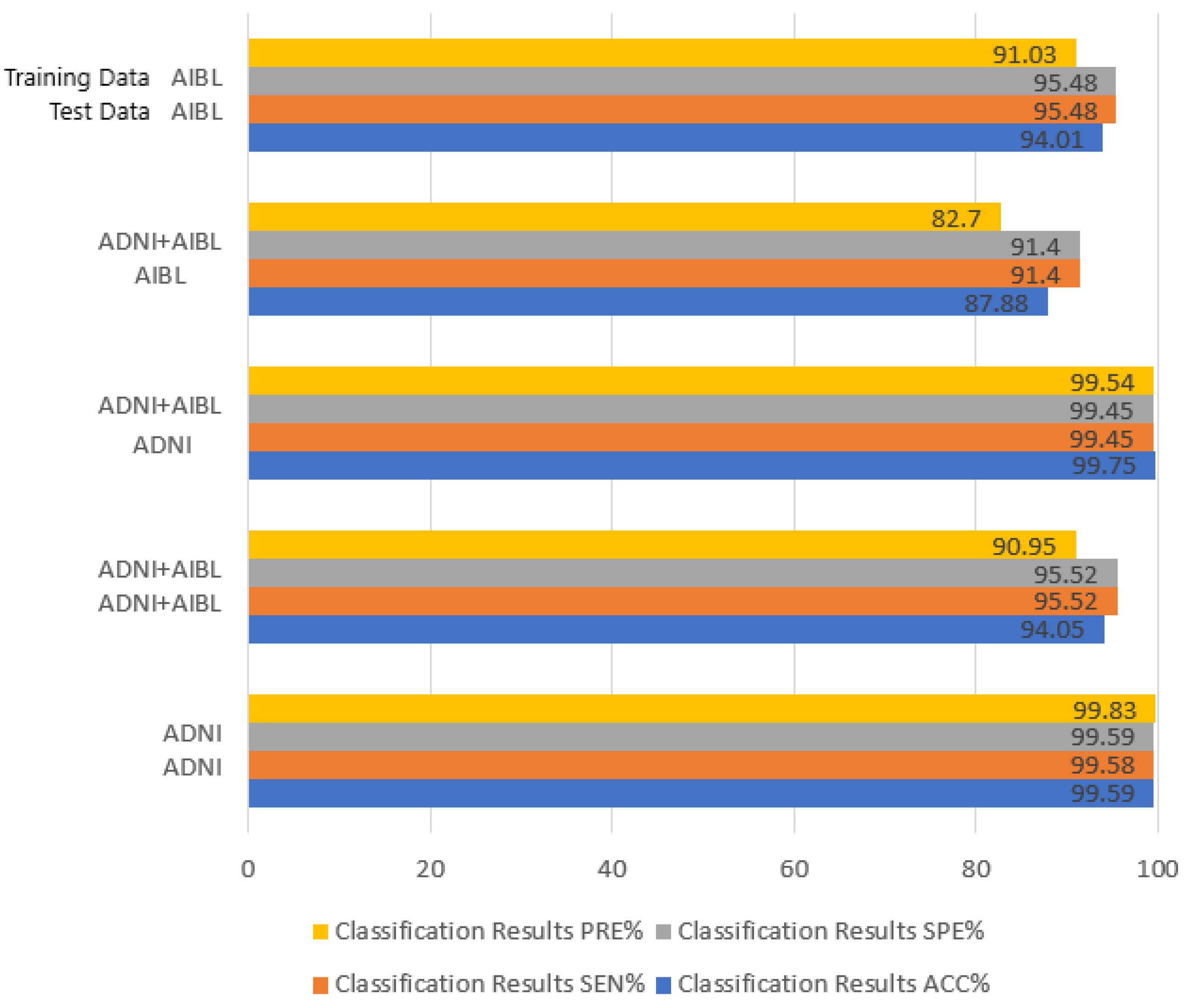
4.3. Experimental Results

The classification performance was assessed using the following four common specificity indicators: accuracy (ACC), sensitivity (SEN), specificity (SPE), and precision (PRE). True positive, true negative, false positive, and false negative are labeled TP, TN, FP, and FN. Then, ACC, SEN, SPE, and PRE can be expressed as

$$\mathrm{A}\mathrm{C}\mathrm{C}=\frac{\mathrm{T}\mathrm{P}+\mathrm{T}\mathrm{N}}{\mathrm{T}\mathrm{P}+\mathrm{F}\mathrm{P}+\mathrm{T}\mathrm{N}+\mathrm{F}\mathrm{N}}$$

$$\mathrm{S}\mathrm{E}\mathrm{N}=\frac{\mathrm{T}\mathrm{P}}{\mathrm{T}\mathrm{P}+\mathrm{F}\mathrm{N}}$$

$$\mathrm{S}\mathrm{P}\mathrm{E}=\frac{\mathrm{T}\mathrm{N}}{\mathrm{T}\mathrm{N}+\mathrm{F}\mathrm{P}}$$

$$\mathrm{P}\mathrm{R}\mathrm{E}=\frac{\mathrm{T}\mathrm{P}}{\mathrm{T}\mathrm{P}+\mathrm{F}\mathrm{P}}$$

(5)

In order to demonstrate the superiority of this method, we compared various studies of different types in this field on ADNI public datasets, as shown in

Table 2. Comparison of our proposed model with related studies.

Models	Types	Classification Results
		ACC%	SEN%	SPE%	PRE%
DenseCNN [12]	ROI	89.80	98.50	85.20	--
CNN [17]	Whole	93.00	92.00	94.00	--
LDMIL [19]	Patch	92.02 ± 0.93	90.76 ± 2.72	92.40 ± 1.10	--
ResNet+Attention [20]	Attention	90.00	92.80	87.50	--
ResNet+ViT [22]	Transformer	92.26	88.98	94.04	--
CNN+ViT [23]	Transformer	90.58	--	--	--
CNN+ViT [24]	Transformer	96.80	--	--	97.20
Ours	Transformer	99.59	99.58	99.59	99.83

The abbreviations of the models are taken from the corresponding research. ROI means the model is based on the region of interest (ROI), and the rest are similar. Accuracy (ACC), sensitivity (SEN), specificity (SPE), and precision (PRE) are the four indicators used to assess the classification performance. The bold denotes our method.

. Experimental results show that our method has excellent performance. At the same time, we compared studies based on Transformers. These studies also performed well, benefiting from the ability of Transformers to capture distant information. Compared with the research in [21], which also combines transfer learning technology, the performance of the RST architecture is significantly improved. It can be seen that our proposed RST architecture can effectively classify AD and NC.

4.4. Ablation Experiments

We carried out several ablation experiments to maximize the experimental outcomes.

Experiment 1: We used sMRI slices in three different orientations. In

Table 3. Comparisons of three directional slices using RST model.

Types	Classification Results
	ACC%	SEN%	SPE%	PRE%
Sagittal	99.69	99.74	99.67	99.54
Coronal	99.07	99.46	98.79	98.50
Axial	99.59	99.58	99.59	99.83

, the experimental findings are displayed. The worst result was obtained when using the coronal plane slice without the skull-stripping preprocessing procedure, which differed greatly from the findings of the other two orientations. Since most experiments were centered on the axial plane and the differences between the experimental outcomes in the axial and sagittal planes were not particularly apparent, axial plane slices were employed in this experiment.

Experiment 2: Tests were run to show how well the various parts of our proposed RST model worked together. The test results are listed in

Table 4. Comparison of different data types and network structures.

Models	Data	ACC
RST	No skull stripping	98.74%
RST	2.5D skull stripping	96.36%
RST	Skull stripping	98.99%
CNN+RST	Skull stripping	99.98%
ST	No skull stripping	95.87%
CNN+ST	No skull stripping	98.87%
CNN+RST	No skull stripping	99.62%

RST: ReSwin Transformer; ST: Swin Transformer. The input consists of axial, sagittal, and coronal sMRI slices, called 2.5D data. The bold denotes the best results.

. The RST model, as implemented by a CNN, performs noticeably better than the other experiments, as shown in the table. In contrast, the step of skull stripping only slightly improves the performance of the RST model and is not proportional to the additional expense it incurs. We used sMRI’s axial, sagittal, and coronal slices as the three input channels of the RST model, but surprisingly, the RST model did not perform well on 2.5D image data. Our analysis results may be due to 2.5D images containing more information, and the model cannot effectively extract features from them. At the same time, we also conducted a comparison with the Swin Transformer, and the experimental results show that the RST is still superior to the Swin Transformer on the ADNI dataset.

Experiment 3: Investigations were carried out on several datasets to confirm the robustness of our proposed model. The outcomes of our trials are shown in Figure 6. The table illustrates that our model performs better for various datasets. The analysis results may be caused by the unevenness of the datasets and the image discrepancies between the datasets because the findings of AIBL, on the other hand, are worse than those of ADNI.

5. Conclusions and Future Work

This paper presents a Resizer Swin Transformer architecture that combines cross-channel learning with a CNN and extracts features from two-dimensional axial-plane slices of brain MRI. The analysis and visualization of the experimental data demonstrated the accuracy with which the RST architecture can accomplish the categorization of AD, as well as its strong adaptability to various datasets. This experiment does still have some flaws, though. The RST model has comparatively high model parameters, and cross-channel learning in conjunction with the CNN enhances the classification performance using the model. Meanwhile, we discovered that the accuracy of the experimental findings is lower than 85% when the model trained on ADNI is directly assessed using AIBL. The model may undergo further development to overcome these problems and provide a lighter and more scalable model. And we hope that in the future, we can better connect image preprocessing with the deep-learning model to construct an end-to-end model that can actually be used in clinical diagnosis.

References

1. Ahmed, S.T.; Kumar, V.; Kim, J. AITel: eHealth Augmented Intelligence based Telemedicine Resource Recommendation Framework for IoT devices in Smart cities. IEEE Internet Things J. 2023. [Google Scholar] [CrossRef]
2. Burgos, N.; Colliot, O. Machine learning for classification and prediction of brain diseases: Recent advances and upcoming challenges. Curr. Opin. Neurol. 2020, 33, 439–450. [Google Scholar] [CrossRef] [PubMed]
3. Segato, A.; Marzullo, A.; Calimeri, F.; De Momi, E. Artificial intelligence for brain diseases: A systematic review. APL Bioeng. 2020, 4, 041503. [Google Scholar] [PubMed]
4. Cai, L.; Gao, J.; Zhao, D. A review of the application of deep learning in medical image classification and segmentation. Ann. Transl. Med. 2020, 8, 1–15. [Google Scholar] [CrossRef] [PubMed]
5. Ahmed, S.T.; Koti, M.S.; Muthukumaran, V.; Joseph, R.B. Interdependent Attribute Interference Fuzzy Neural Network-Based Alzheimer Disease Evaluation. Int. J. Fuzzy Syst. Appl. (IJFSA) 2022, 11, 1–13. [Google Scholar] [CrossRef]
6. Vemuri, P.; Jack, C.R. Role of structural MRI in Alzheimer’s disease. Alzheimer’s Res. Ther. 2010, 2, 23. [Google Scholar] [CrossRef]
7. Dharwada, S.; Tembhurne, J.; Diwan, T. Multi-channel Deep Model for Classification of Alzheimer’s Disease Using Transfer Learning. In Proceedings of the Distributed Computing and Intelligent Technology: 18th International Conference, ICDCIT 2022, Bhubaneswar, India, 19–23 January 2022; Springer International Publishing: Cham, Switzerland, 2022; pp. 245–259. [Google Scholar]
8. Yamanakkanavar, N.; Choi, J.Y.; Lee, B. MRI segmentation and classification of human brain using deep learning for diagnosis of Alzheimer’s disease: A survey. Sensors 2020, 20, 3243. [Google Scholar] [CrossRef]
9. Druzhinina, P.; Kondrateva, E. The effect of skull-stripping on transfer learning for 3D MRI models: ADNI data. In Proceedings of the Medical Imaging with Deep Learning 2022, Zürich, Switzerland, 6–8 July 2022. [Google Scholar]
10. Liu, Z.; Lin, Y.; Cao, Y.; Hu, H.; Wei, Y.; Zhang, Z.; Lin, S.; Guo, B. Swin transformer: Hierarchical vision transformer using shifted windows. In Proceedings of the IEEE/CVF International Conference on Computer Vision, Montreal, QC, Canada, 10–17 October 2021; pp. 10012–10022. [Google Scholar]
11. Hu, Z.; Wang, Z.; Jin, Y.; Hou, W. VGG-TSwinformer: Transformer-based deep learning model for early Alzheimer’s disease prediction. Comput. Methods Programs Biomed. 2023, 229, 107291. [Google Scholar] [CrossRef]
12. Zou, L.; Lam, H.F.; Hu, J. Adaptive resize-residual deep neural network for fault diagnosis of rotating machinery. Struct. Health Monit. 2023, 22, 2193–2213. [Google Scholar] [CrossRef]
13. Zhang, R.; Isola, P.; Efros, A. Colorful image colorization. In Proceedings of the Computer Vision–ECCV 2016: 14th European Conference, Amsterdam, The Netherlands, 11–14 October 2016; Proceedings, Part III 14. Springer International Publishing: Cham, Switzerland, 2016; pp. 649–666. [Google Scholar]
14. Wang, Q.; Li, Y.; Zheng, C.; Xu, R. DenseCNN: A Densely Connected CNN Model for Alzheimer’s Disease Classification Based on Hippocampus MRI Data. In AMIA Annual Symposium Proceedings; American Medical Informatics Association: Bethesda, MD, USA, 2020; Volume 2020, p. 1277. [Google Scholar]
15. Pan, D.; Zou, C.; Rong, H.; Zeng, A. Early diagnosis of Alzheimer’s disease based on three-dimensional convolutional neural networks ensemble model combined with genetic algorithm. J. Biomed. Eng. 2021, 38, 47–55. [Google Scholar]
16. Huang, H.; Zheng, S.; Yang, Z.; Wu, Y.; Li, Y.; Qiu, J.; Wu, R. Voxel-based morphometry and a deep learning model for the diagnosis of early Alzheimer’s disease based on cerebral gray matter changes. Cereb. Cortex 2023, 33, 754–763. [Google Scholar] [CrossRef] [PubMed]
17. Hazarika, R.A.; Kandar, D.; Maji, A.K. An experimental analysis of different deep learning-based models for Alzheimer’s disease classification using brain magnetic resonance images. J. King Saud Univ.-Comput. Inf. Sci. 2022, 34, 8576–8598. [Google Scholar] [CrossRef]
18. Morid, M.A.; Borjali, A.; Del Fiol, G. A scoping review of transfer learning research on medical image analysis using ImageNet. Comput. Biol. Med. 2021, 128, 104115. [Google Scholar] [CrossRef]
19. Zhang, F.; Pan, B.; Shao, P.; Liu, P.; Shen, S.; Yao, P.; Xu, R.X. An explainable two-dimensional single model deep learning approach for Alzheimer’s disease diagnosis and brain atrophy localization. arXiv 2017, arXiv:2107.13200. [Google Scholar]
20. Liu, M.; Zhang, J.; Nie, D.; Yap, P.T.; Shen, D. Anatomical landmark based deep feature representation for MR images in brain disease diagnosis. IEEE J. Biomed. Health Inform. 2018, 22, 1476–1485. [Google Scholar] [CrossRef] [PubMed]
21. Liu, M.; Zhang, J.; Adeli, E.; Shen, D. Landmark-based deep multi-instance learning for brain disease diagnosis. Med. Image Anal. 2018, 43, 157–168. [Google Scholar] [CrossRef]
22. Zhang, Y.; Teng, Q.; Liu, Y.; Liu, Y.; He, X. Diagnosis of Alzheimer’s disease based on regional attention with sMRI gray matter slices. J. Neurosci. Methods 2022, 365, 109376. [Google Scholar] [CrossRef]
23. Han, K.; Xiao, A.; Wu, E.; Guo, J.; Xu, C.; Wang, Y. Transformer in transformer. Adv. Neural Inf. Process. Syst. 2021, 34, 15908–15919. [Google Scholar]
24. Li, C.; Cui, Y.; Luo, N.; Liu, Y.; Bourgeat, P.; Fripp, J.; Jiang, T. Trans-ResNet: Integrating Transformers and CNNs for Alzheimer’s disease classification. In Proceedings of the 2022 IEEE 19th International Symposium on Biomedical Imaging (ISBI), Kolkata, India, 28–31 March 2022; pp. 1–5. [Google Scholar]
25. Jang, J.; Hwang, D. M3T: Three-dimensional Medical image classifier using Multi-plane and Multi-slice Transformer. In Proceedings of the IEEE/CVF Conference on Computer Vision and Pattern Recognition, New Orleans, LA, USA, 18–24 June 2022; pp. 20718–20729. [Google Scholar]
26. Deng, J.; Dong, W.; Socher, R.; Li, L.J.; Li, K.; Fei-Fei, L. Imagenet: A large-scale hierarchical image database. In Proceedings of the 2009 IEEE Conference on Computer Vision and Pattern Recognition, Miami, FL, USA, 20–25 June 2009; pp. 248–255. [Google Scholar]
27. Lyu, Y.; Yu, X.; Zhu, D.; Zhang, L. Classification of Alzheimer’s Disease via Vision Transformer: Classification of Alzheimer’s Disease via Vision Transformer. In Proceedings of the 15th International Conference on PErvasive Technologies Related to Assistive Environments, Corfu, Greece, 29 June–1 July 2022; pp. 463–468. [Google Scholar]
28. Zhang, Z.; Gong, Z.; Hong, Q.; Jiang, L. Swin-transformer based classification for rice diseases recognition. In Proceedings of the 2021 International Conference on Computer Information Science and Artificial Intelligence (CISAI), Kunming, China, 17–19 September 2021; pp. 153–156. [Google Scholar]
29. Nawaz, W.; Ahmed, S.; Tahir, A.; Khan, H.A. Classification of breast cancer histology images using alexnet. In Proceedings of the Image Analysis and Recognition: 15th International Conference, ICIAR 2018, Póvoa de Varzim, Portugal, 27–29 June 2018; Proceedings 15. Springer International Publishing: Cham, Switzerland; pp. 869–876. [Google Scholar]
30. Sarwinda, D.; Paradisa, R.H.; Bustamam, A.; Anggia, P. Deep learning in image classification using residual network (ResNet) variants for detection of colorectal cancer. Procedia Comput. Sci. 2021, 179, 423–431. [Google Scholar] [CrossRef]
31. Marques, G.; Agarwal, D.; de la Torre Díez, I. Automated medical diagnosis of COVID-19 through EfficientNet convolutional neural network. Appl. Soft Comput. 2020, 96, 106691. [Google Scholar] [CrossRef]
32. Wang, Y.; Yan, W.Q. Colorizing Gray-scale CT images of human lungs using deep learning methods. Multimed. Tools Appl. 2022, 81, 37805–37819. [Google Scholar] [CrossRef] [PubMed]
33. Talebi, H.; Milanfar, P. Learning to resize images for computer vision tasks. In Proceedings of the IEEE/CVF International Conference on Computer Vision, Montreal, QC, Canada, 10–17 October 2021; pp. 497–506. [Google Scholar]
34. Petersen, R.C.; Aisen, P.S.; Beckett, L.A.; Donohue, M.C.; Gamst, A.C.; Harvey, D.J.; Weiner, M.W. Alzheimer’s disease neuroimaging initiative (ADNI): Clinical characterization. Neurology 2010, 74, 201–209. [Google Scholar] [CrossRef] [PubMed]
35. Ellis, K.A.; Bush, A.I.; Darby, D.; De Fazio, D.; Foster, J.; Hudson, P.; AIBL Research Group. The Australian Imaging, Biomarkers and Lifestyle (AIBL) study of aging: Methodology and baseline characteristics of 1112 individuals recruited for a longitudinal study of Alzheimer’s disease. Int. Psychogeriatr. 2009, 21, 672–687. [Google Scholar] [CrossRef] [PubMed]
Figure 1. The overall structure of the proposed model. The CNN module is used to convert a single-channel gray-scale image of the axial sMRI slices into a three-channel RGB image. The Resizer module resizes the input image and removes invalid parts. The Swin Transformer identifies features that are useful for classification. Finally, the Softmax layer generates classification scores for each slice.
Applsci 13 09310 g001
Figure 2. Colorization CNN network structure. The numbers and cubes of different colors are the feature map and C × H × W of the feature map after a series of convolution operations; Blocks 1, 2, and 3 show the specific details of the convolution operation corresponding to the blue, yellow, and orange feature maps, respectively. Given the lightness channel L of a gray-scale image, this model predicts the corresponding a and b color channels of the image in the CIE Lab color space. Finally, it is converted to the RGB color space, and the image is output.
Applsci 13 09310 g002
Figure 3. Resizer module in our proposed model for resizing images. The original size of the image is (181, 217), and the bilinear Resizer up-samples the image to a size of (224, 224) as the input for the Swin Transformer.
Applsci 13 09310 g003
Figure 4. Swin Transformer and its block structure. (a) The overall structure of the Swin Transformer. A Swin Transformer block contains two attention calculations. The specific computation process is shown in (b).
Applsci 13 09310 g004
Figure 5. (ac) The variation in ACC with epoch for different batch sizes with learning rates of 1 × 10⁻⁵, 5 × 10⁻⁵, and 1 × 10⁻⁶, respectively. (d) Comparison of the two curves with the optimal variation in ACC.
Applsci 13 09310 g005
Figure 6. Experimental results of RST on different datasets. The left horizontal coordinate represents the experimental results obtained under the corresponding training set and test set.
Applsci 13 09310 g006