1. Introduction
The Industrial Control System (ICS) serves as the backbone of the Industrial Internet, which in turn is the product of the combination of new-generation technologies such as communication and automation with traditional industrial networks in the 21st century [
1]. Industrial control systems are an important part of industrial development, controlling the operation of different working systems in different industries and building a digital, networked industrial chain through the connection of field devices, operators, and other facilities. It is an important cornerstone of Industry 4.0 [
2]. Network security has always been a key concern, and the security of industrial control systems needs to be given the same high priority [
3]. The Purdue model, which is now the reference standard for industrial control system security, demonstrates the interdependence of all the components of a typical ICS and is an important reference point for starting to build a typical modern ICS architecture. The Purdue model is shown in
Figure 1. The intrusion detection system is a very important part of the computer network system; its purpose is to collect key useful information from different parts of the network system and, by analyzing the collected data, determine whether there are insecure behaviors in the current network system that cause damage to the network. Compared with traditional network defense mechanisms such as firewalls, VNPs, access control, etc., network intrusion detection systems can detect some unknown means of attack [
4,
5]. At the same time, intrusion detection systems can detect attacks without affecting network performance and achieve real-time protection of network systems [
6,
7].
Intrusion detection systems commonly use two analysis methods, anomaly detection and misuse detection, to detect and analyze abnormal behavior. As deep learning technology advances, progresses, and evolves, people are gradually combining deep learning algorithms and industrial control system intrusion detection to find more suitable methods to protect the system.
Compared with traditional machine learning algorithms, deep learning can mine more advanced and important features in massive data. Akashdeep Bhardwaj et al. [
8] introduced a pattern recognition algorithm named “Capture the Invisible (CTI)”. Used to find hidden processes in industrial control device logs and detect behavior-based attacks executed in real-time. Yongle Chen et al. [
9] developed a method to improve the information transfer link in adversarial domain adaptation (DA). This approach is capable of training the anomaly detection depth using unbalanced data. Experiments have high detection accuracy on SCADA network layer-based data. Khan, M.A. [
10] creating a deep learning-based hybrid intrusion detection framework by convolutional recurrent neural network (CRNN) using convolutional neural network (CNN) to capture local features and recurrent neural network (RNN) to capture temporal features to improve the performance of the intrusion detection system, the effectiveness of the model is validated on the CSE-CIC-DS2018 dataset. Yan Hu et al. [
11] proposed a new alignment entropy-based method to detect stealth attacks on ICSs, by which the non-randomness contained in the residuals can be characterized, thus effectively distinguishing the residuals from random sequences during stealth attacks. The experiments were synthesized in the Matlab-Simulink environment, and the results verified excellent detection capabilities. Jie Ling et al. [
12] proposed an intrusion detection method based on bi-directional simple recursive units (BiSRU). It was also validated on two standard industrial datasets at Mississippi State University, and the results showed that the proposed method is more accurate and requires less training time. Chao Wang et al. [
13] proposed a self-encoder-based intrusion detection method for industrial control systems that simultaneously predicts and reconstructs the input data, thus overcoming the drawback of using each data individually. Using the errors obtained from the model, a rate of change is proposed to locate the most likely suspect devices under attack. Experiments were conducted on the SWaT dataset to verify the high validity of the method.
The above research is based on the deep learning method of supervised learning; however, supervised learning requires labeled data to train the model, so a large amount of data is needed to support the training of the model [
14]. In industrial control systems, communication data is the object of study, and normal or abnormal traffic occurs in the process of system operation, in which there may be uneven data distribution and unknown data traffic. Most of these data need to be manually labeled to distinguish, and if these unlabeled data cannot be used well, it will bring trouble to the intrusion detection system. Contrast learning belongs to self-supervised learning, which in turn is the category of unsupervised learning [
15]. Contrast learning enables the use of unlabeled data to assist in training a feature extraction network and improve the accuracy of subsequent classification detection tasks. The classical algorithms for contrast learning include SimCLR, Momentum Contrast for Unsupervised Visual Representation Learning (MoCo), Bootstrap Your Own Latent: A New Approach to Self-Supervised Learning (BYOL), Exploring Simple Siamese Representation Learning (SimSiam), Swapping Assignments between Multiple Views of the Same Image (SWaV) [
16,
17,
18,
19,
20], etc.
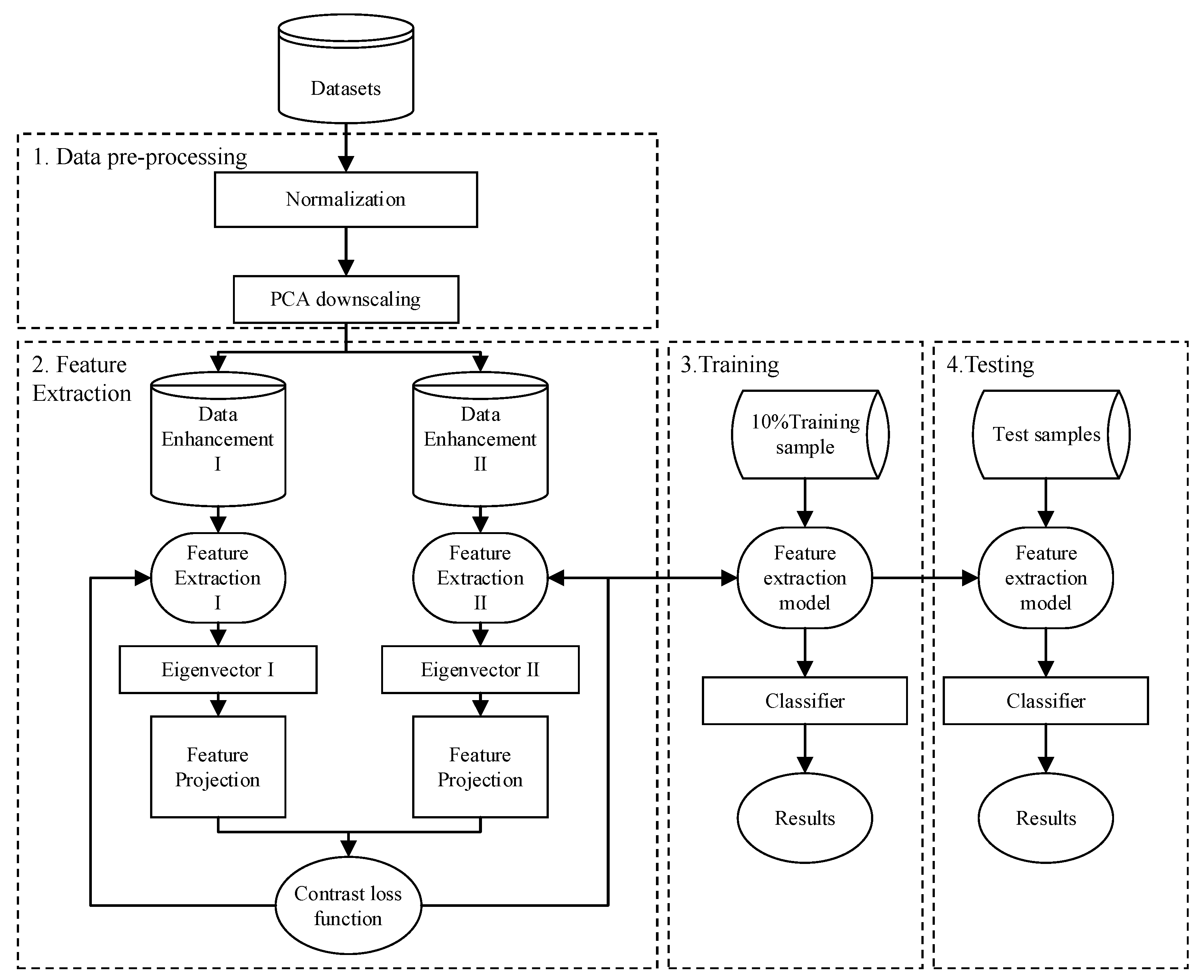
In this paper, we propose an intrusion detection model for industrial control systems based on the improved comparative learning model SimCLR by combining the improved comparative learning model SimCLR with industrial control system intrusion detection. Firstly, we need to perform data pre-processing on the obtained industrial control traffic data, use normalization to map the data to the 0-1 interval to eliminate the adverse effects caused by odd sample data, and use the principal component analysis (PCA) algorithm for dimensionality reduction on the normalized data, which can effectively reduce the data dimensionality, eliminate redundant information, and improve the efficiency of data processing and data quality. Unlike the supervised model, the contrast learning model does not require the use of labeled data to train the network model. It is a self-supervised learning method that allows the model to learn which data points are similar or which data points are different to learn the general characteristics of the data set without the data being labeled. The contrast learning model has four main phases: data augmentation, feature extraction, feature projection, and the calculation of contrast loss. The trained contrast learning feature extraction network is transferred to the supervised learning training, and the model is fine-tuned by using only 10% of the labeled data in the simulated experimental dataset. Finally, the trained model is tested on the test data.
The innovative points of this paper are as follows:
- (1)
An intrusion detection model for industrial control systems based on improved comparative learning SimCLR is proposed, and the data enhancement is improved by adding random noise, sequence inversion, and random sampling of the Synthetic Minority Over-sampling Technique (SMOTE) algorithm to the original industrial control traffic data. The other one uses only the SMOTE algorithm. The other one uses only the SMOTE algorithm to replace the original data with the same multiplicity of sampling.
- (2)
The asymmetric network structure is adopted on top of the original model, which enables different networks to perform feature extraction for different types of data.
- (3)
The feature projection structure is improved by using feature cross-fusion to cross-fuse two feature vectors and using a jump join between the first and last linear layer to add the two vectors before and after the projection, which increases the similarity between positive and negative examples and makes the similarity between positive and negative examples more distant.
The article is structured as follows:
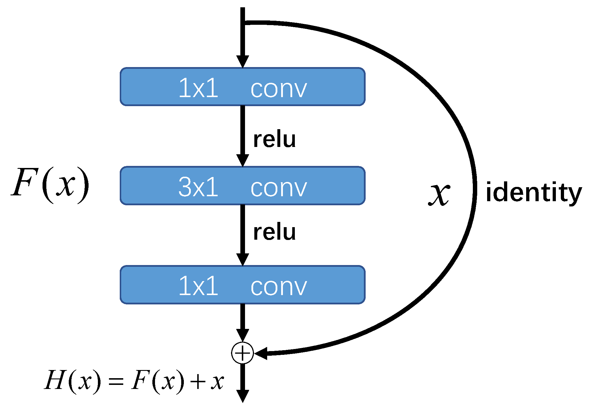
Section 2 introduces the SMOTE algorithm and the deep residual network, ResNet.
Section 3 presents the proposed intrusion detection model based on contrast learning for industrial control systems.
Section 4 presents the datasets used in the experiments, the model evaluation metrics, and the experimental results.
Section 5 summarizes the work of this paper and provides an outlook for the future.
4. Experiments and Results Analysis
The experiments divide the data into unlabeled data for training the feature extraction network in the contrast learning model and labeled training and test data for supervised training of the fine-tuned model. Firstly, comparison experiments between different temperature coefficients are conducted to select the best temperature coefficients for contrast learning. The effectiveness of this method is verified by comparing the experimental results between different data enhancement methods and this method. A contrast learning feature extraction network trained with unlabeled data is added with a linear classification layer, and a small amount of labeled training data is used to compare the classification results with other deep learning models through model fine-tuning to verify the effectiveness of this method. Finally, the SWaT dataset was replaced and tested using the present model to further validate the applicability of the model.
4.1. Experimental Data Set
The intrusion detection dataset for the industrial control system used in this experiment was obtained from Mississippi State University. The researchers examined and captured the natural gas pipeline control system traffic data through a network data logger and obtained 97,019 experimental datasets. The data contains pre-processed network transaction data with the underlying transport data (TCP, MAC, etc.) removed. Each data entry contains 26 traffic attributes and one attack category, where the attack category has seven attack types and one normal type. The attack types and label descriptions are shown in
Table 3. The distribution of sample size is shown in
Figure 7.
4.2. Model Evaluation Metrics
In this experiment, four metrics were adopted to evaluate the model: Accuracy, Precision, Recall, and F1, in which several basic concepts need to be introduced:
TP (True Positive): The prediction is positive, and the actual case is positive.
FP (False Positive): Predicted positive case, actual negative case.
FN (False Negative): Predicted negative case, actual positive case.
TN (True Negative): The predicted case is negative, and the actual case is negative.
Accuracy rate: It indicates the percentage of all correctly classified samples in the total number of samples. The specific calculation formula is shown in Equation (
12):
Precision rate: indicates the percentage of correct predictions that are positive among all predictions that are positive. The specific calculation formula is shown in Equation (
13):
Recall: indicates the percentage of correct predictions that are positive in all actual positive. The specific calculation formula is shown in Equation (
14):
: The calculation formula is shown in Equation (
15):
4.3. Parameter Setting
The system environment used for this experiment is the Windows 10 operating system; the CPU model of the computer is I7-11800H; the GPU model is Geforce GTX 2080Ti; the system running memory is 16 Gb; and the model is built using the deep learning framework Pytorch 1.10. The experimental part of the model needs to select the appropriate Batch_size, learning rate, and optimizer, and the most appropriate learning rate, optimizer, and Batch_size are selected by experimental comparison, and the experimental results are shown in
Figure 8,
Figure 9 and
Figure 10, respectively.
The experiments use training accuracy as an evaluation metric, and the best learning rate is 0.001, the best optimizer is Adam, and the best batch size is 256, as derived from
Figure 8,
Figure 9 and
Figure 10.
4.4. Experimental Results and Analysis
4.4.1. Comparison of Experimental Results with Different Temperature Coefficients
The temperature coefficient plays an important role in the process of comparison loss calculation, and by changing the size of the temperature coefficient, the degree of attention to difficult samples can be adjusted. In general, the smaller the temperature coefficient, the more attention is paid to separating positive samples from other samples and, thus, whether better classification can be achieved. The temperature coefficients of 0.5, 0.2, and 0.07 were used to derive the change curves of contrast loss values with an increasing number of iterations, as shown in
Figure 11.
As can be seen from
Figure 11, the contrast loss is minimized when using a temperature coefficient of 0.07 and maximized when the temperature coefficient is 0.5. The smaller the temperature coefficient, the stronger the contrast learning effect, and the more you can distinguish between positive and negative samples.
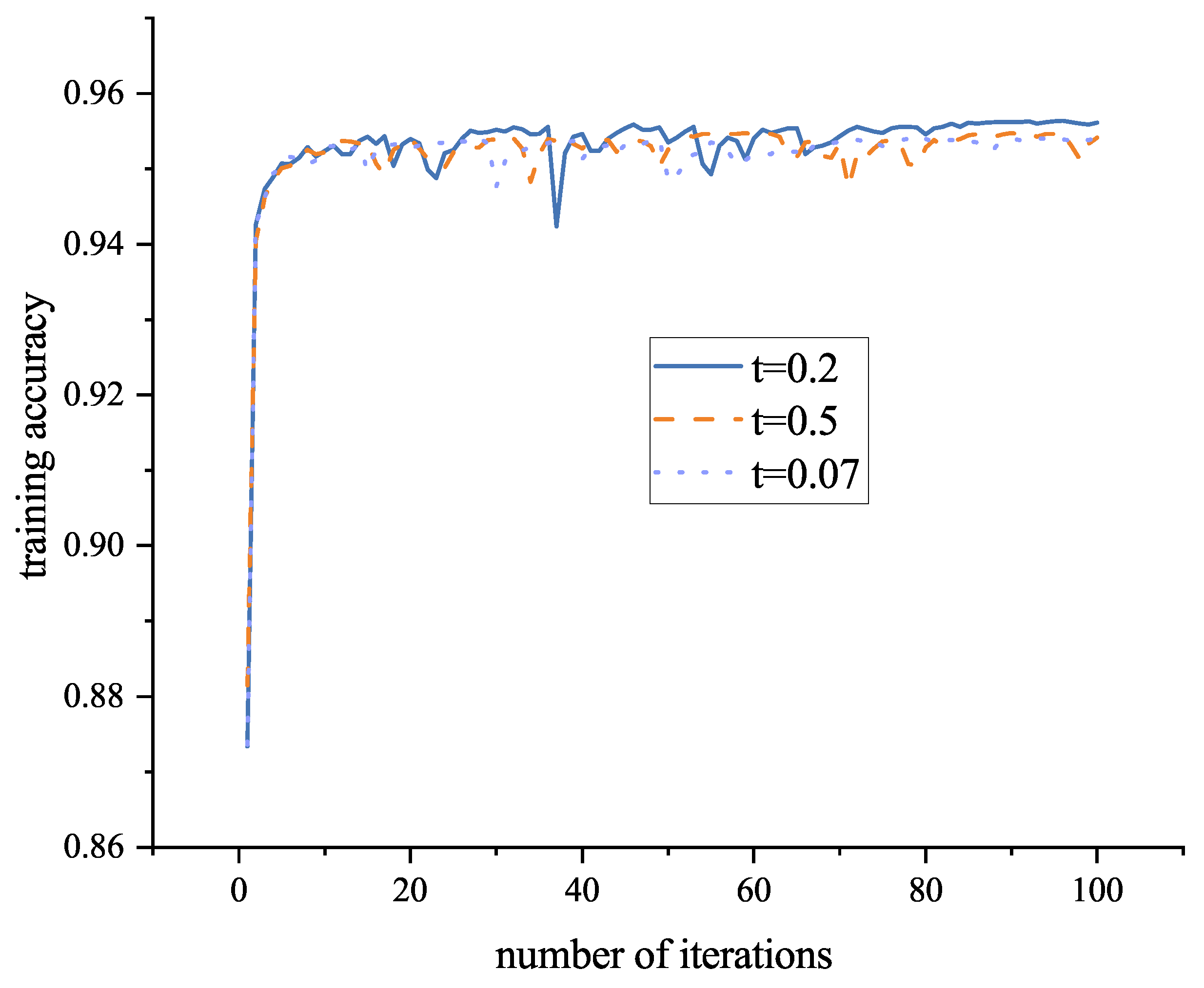
Then the feature extraction network was trained using the temperature coefficients of 0.5, 0.2, and 0.07, respectively, and the accuracy of the model training for 100 batches is shown in
Figure 12 by training the classification behind the network by adding a fully connected layer.
As can be seen from
Figure 12, the highest accuracy and best training results are achieved when the temperature coefficient is chosen to be 0.2. In this case, the negative samples that are extremely similar to the positive samples are often likely to be potential positive samples, and the larger the temperature coefficient, the more there is no difference for the comparison between positive and negative samples, which tend to be treated equally and do not pay too much attention to the more difficult negative samples, so too large or too small temperature coefficients are not conducive to the calculation of contrast loss.
4.4.2. Comparison of Experimental Results of Different Data Enhancement Methods
To validate the efficacy of the data augmentation technique proposed in this paper, the SMOTE algorithm sampling, adding Gaussian noise, sequence inversion, and the original data were selected for comparison learning experiments with the data channel fusion method in this paper, respectively. Firstly, different data enhancements were performed on the basis of obtaining the original industrial control data traffic, and the sequence distribution after using different data enhancements is shown in
Figure 13.
It can be seen from
Figure 13 that the feature distribution of the data with Gaussian noise added and the data sampled with the SMOTE algorithm is not much different from the original data. The feature distribution of the data after the sequence inversion is opposite to the original data.
The experimental accuracy of the comparison learning model training after using different data enhancements is shown in
Figure 14.
The experimental results show that the data with channel merging are better than those with SMOTE sampling, Gaussian noise addition, sequence inversion, and the original data. The data with sequence inversion differed from the original data in dimensional order, and the experimental results were worse than the other three. The data after channel merging incorporates data enhanced by different types of data and has higher-order features of multiple data types, which can obtain better features after subsequent feature extraction and improve the classification detection effect.
4.4.3. Comparison of Experimental Results of Different Classification Models
On top of the trained contrast learning model, the feature extraction network is obtained, a linear classification layer is added and retrained using a small amount of labeled data, and the classification experiment is completed by fine-tuning the model parameters. CNN and LSTM are commonly used deep learning algorithms. The results of this model are compared with three algorithms after improvement: ResNet, CNN-LSTM, and Attention-LSTM, which are deep learning methods without using comparison learning models for training assistance. The loss values and accuracy curves of the models in the training phase are shown in
Figure 15 and
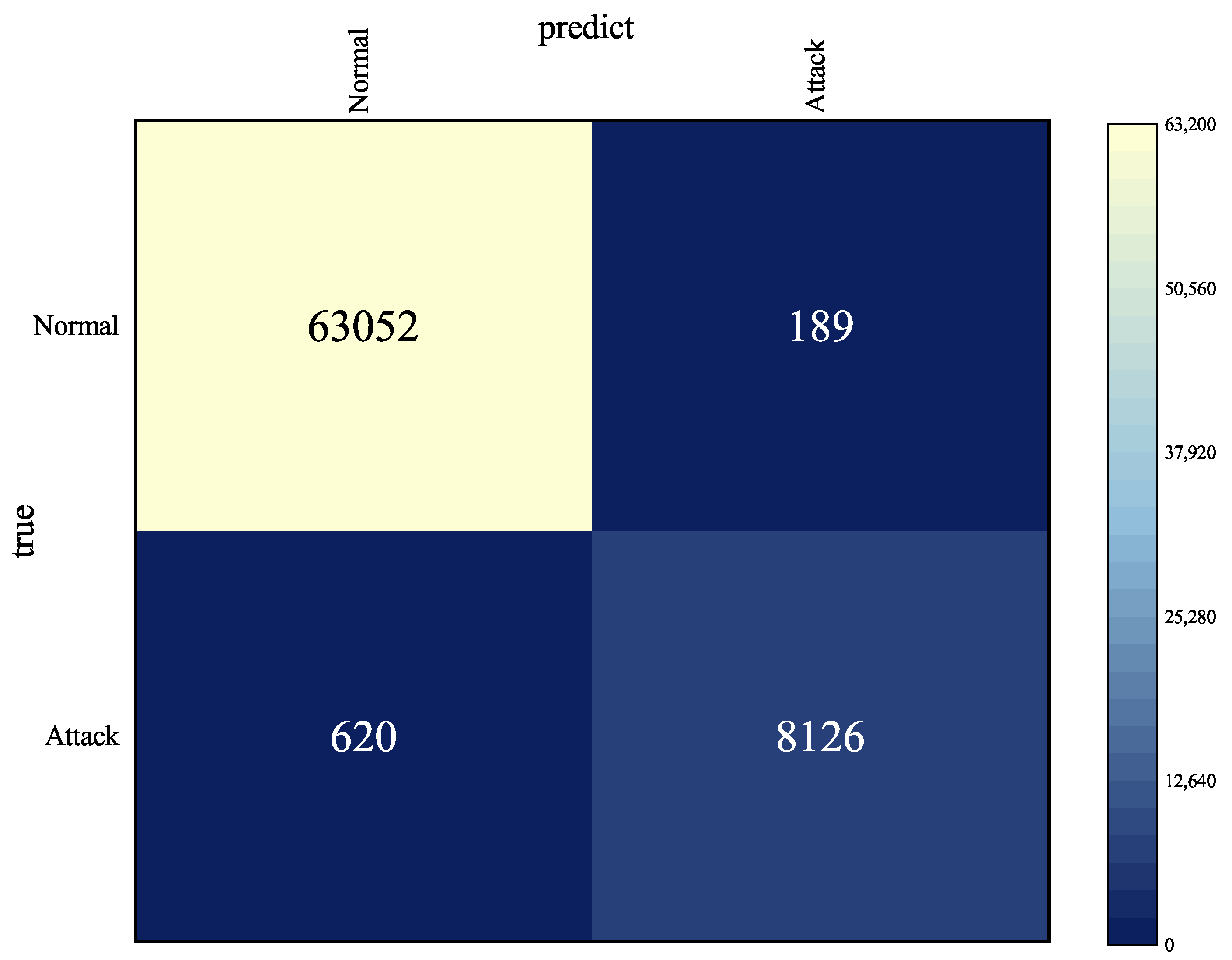
Figure 16, the confusion matrix of the test set results is shown in
Figure 17, and the evaluation metrics of the four models are shown in
Table 4.
From
Figure 15 and
Figure 16, it can be seen that the model training on the training set, as the number of training iterations increases, has the highest accuracy and the smallest loss value. From the confusion matrix in
Figure 17; it can be seen that most of the results are located on the diagonal of the matrix, and a small number of results are located on both sides of the diagonal, indicating that the model is able to detect most of the results. As can be seen from
Table 4, using the test set in the trained model for model testing, the method in this paper achieves 95.7%, 98.1%, 94.0%, and 96.0% in the four indexes of accuracy, precision, recall, and F1, respectively. The results are better than ResNet, CNN-LSTM, and Attention-LSTM. The model training time is shown in
Table 5:
4.4.4. Experimental Results for Different Datasets
To verify the applicability of the model, this section further validates its performance by replacing it with the SWaT dataset, using the same experimental approach as described above. Again, the experimental results are compared with three common deep learning algorithms, and the confusion matrix for the experiments as well as the model evaluation metrics are shown in
Figure 18 and
Table 6 below.
From the confusion matrix
Figure 18, we can see that most of the detected results are located on the diagonal of the matrix, which indicates that this model has a better classification effect, and from
Table 6, we can see that the four indexes of accuracy, precision, recall, and F1 in this paper reach 98.9%, 98.4%, 96.3%, and 97.3%, respectively, compared with the other three common deep learning algorithms.


 ,
, 


