
A Novel Gradient-Weighted Voting Approach for Classical and Fuzzy Circular Hough Transforms and Their Application in Medical Image Analysis—Case Study: Colonoscopy

Abstract
:Featured Application
Abstract
1. Introduction
- selecting the edge detection method that is the most suitable for colorectal polyp localization purposes. Developing a metric to base this selection,
- determining gradient limits for removing the unnecessary edges,
- applying fuzzy Hough transform on colonoscopy images and comparing its results with the classical Hough transform,
- introducing a gradient-weighted voting to both classical and fuzzy Hough transforms and study its effects,
- characterizing the roundness of the objects to be detected.
2. Theoretical Background
2.1. Classical and Fuzzy Hough Transforms
- Divide the space by a finite grid (if not already executed).
- Divide the transformed space by a finite grid, it gives the resolution of the result.
- For each point in the transformed space add a vote for each point in the original space, that is contained by the line.
- Search for the maximum of votes
- If there is just one line, the global maximum will be the approximation of parameter of the line we were looking for.
- If there are multiple lines, longer and shorter segments, the local maxima will also approximate parameter pairs of lines.The longer the line in the original space, the more votes it obtains. By setting up a threshold, the length of the detected line segment can be controlled.
- The lines with the detected approximate parameters can be drawn in the original space .
| Algorithm 1: Classical Hough transform for a circle with parameters a, b and r | |
| Requirements: an edge image with size , a finite parameter space with size with initial values of 0 a threshold for peak percentage , a result image , with size , with initial values of 0 | |
| 1: | for each image row from 1 to |
| 2: | for each image column from 1 to |
| 3: | for each parameter space row from 1 to |
| 4: | for each parameter space column from 1 to |
| 5: | for each parameter space 3rd dimension from 1 to |
| 6: | if |
| 7: | |
| 8: | end if |
| 9: | end for |
| 10: | end for |
| 11: | end for |
| 12: | end for |
| 13: | end for |
| 14: | compute the global maximum in |
| 15: | compute local maxima |
| 16: | select local maxima with |
| 17: | calculate the number of the local maxima from line 16 |
| 18: | for each local maximum from 1 to |
| 19: | for each result image row from 1 to |
| 20: | for each result image column from 1 to |
| 21: | if |
| 22: | |
| 23: | end if |
| 24: | end for |
| 25: | end for |
| 26: | end for |
- Divide the space of fuzzy points by a finite grid (if not already executed).
- Divide the transformed space by a finite grid, it gives the resolution of the result.
- For each point in the transformed space, and its environment add a vote proportional to the membership function for each fuzzy point in the original space, that is part of the fuzzy curve.
- Search for the maximum of votes
- If there is just one curve segment, the global maximum will be the approximation of parameter of the curve we were looking for.
- If there are multiple curves, with longer and shorter segments, the local maxima will also approximate parameters of the curves.The longer the curve in the original space, the more votes it obtains. By setting up a threshold the length of the detected segment can be controlled.
- The curves with the detected approximate parameters can be drawn in the original space .
| Algorithm 2: Fuzzy Hough transform for a circle with parameters a, b, and r | |
| Requirements: an edge image with size , a finite parameter space with size , , , with initial values of 0 a threshold for peak percentage , a voting membership matrix with size a result image , with size , with initial values of 0 | |
| 1: | for each image row from 1 to |
| 2: | for each image column from 1 to |
| 3: | for each parameter space row from 1 to |
| 4: | for each parameter space column from 1 to |
| 5: | for each parameter space 3rd dimension from 1 to |
| 6: | if |
| 7: | … |
| 8: | end if |
| 9: | end for |
| 10: | end for |
| 11: | end for |
| 12: | end for |
| 13: | end for |
| 14: | compute the global maximum in |
| 15: | compute local maxima |
| 16: | select local maxima with |
| 17: | calculate the number of the local maxima from line 16 |
| 18: | for each local maximum from 1 to |
| 19: | for each result image row from 1 to |
| 20: | for each result image column from 1 to |
| 21: | if |
| 22: | |
| 23: | end if |
| 24: | end for |
| 25: | end for |
| 26: | end for |
2.2. Gradient Filtering
2.3. The Implemented Edge Detection Algorithms
2.3.1. Roberts, Prewitt, and Sobel Edge Detection Algorithms
2.3.2. Canny Edge Detection Algorithm
3. Practical Application of the Proposed Method
3.1. Edge Detection Methods—Application, Evaluation, and Selection
- Cutting off the black frame surrounding all original images to reduce unnecessary information.
- Removing the colonoscope’s light reflections: The colonoscope light’s reflections (and consequently their contours) were removed from all the databases’ images as a step towards reducing the number of redundant edge pixels (Figure 4b). The histogram of the image pixel intensities was used as the basis for the reflection removal step. Briefly, we cut out the histogram’s highest (and lowest) intensity peaks, and then the pixel intensities were re-normalized to the original [0 to 255] domain. A “white mask” was created using the pixels that made up the histogram’s highest peak. Similar to the procedure described in [49], the “white mask” was extended and smoothened into the neighboring pixels.
- Generating the “ring mask” for the colorectal polyp contour: In many cases of the manually drawn masks, the edges of the polyp’s contour are not completely visible, either because the polyp is located in the area of bowel folds, or it is covered with impurities. Moreover, reasons related to the human fatigue or error can also affect the drawing accuracy of the colorectal polyp mask. These are the main reasons why it was necessary to extend the contour of the manually drawn database mask to a finite width ring which is proportional to the size of the examined image. The previously extracted contour was extended into a ring (Figure 4e). To do that, we selected the first nearest pixels of the entire contour as a width of the ring mask. As the databases images are with different sizes, we used different ring mask widths based on the database images size (they are for CVC-Clinic database [9], for CVC-Colon database [42], and for ETIS-Larib database [34]).
- Calculating the gradient magnitude for each of the studied samples, like in (Figure 4f).
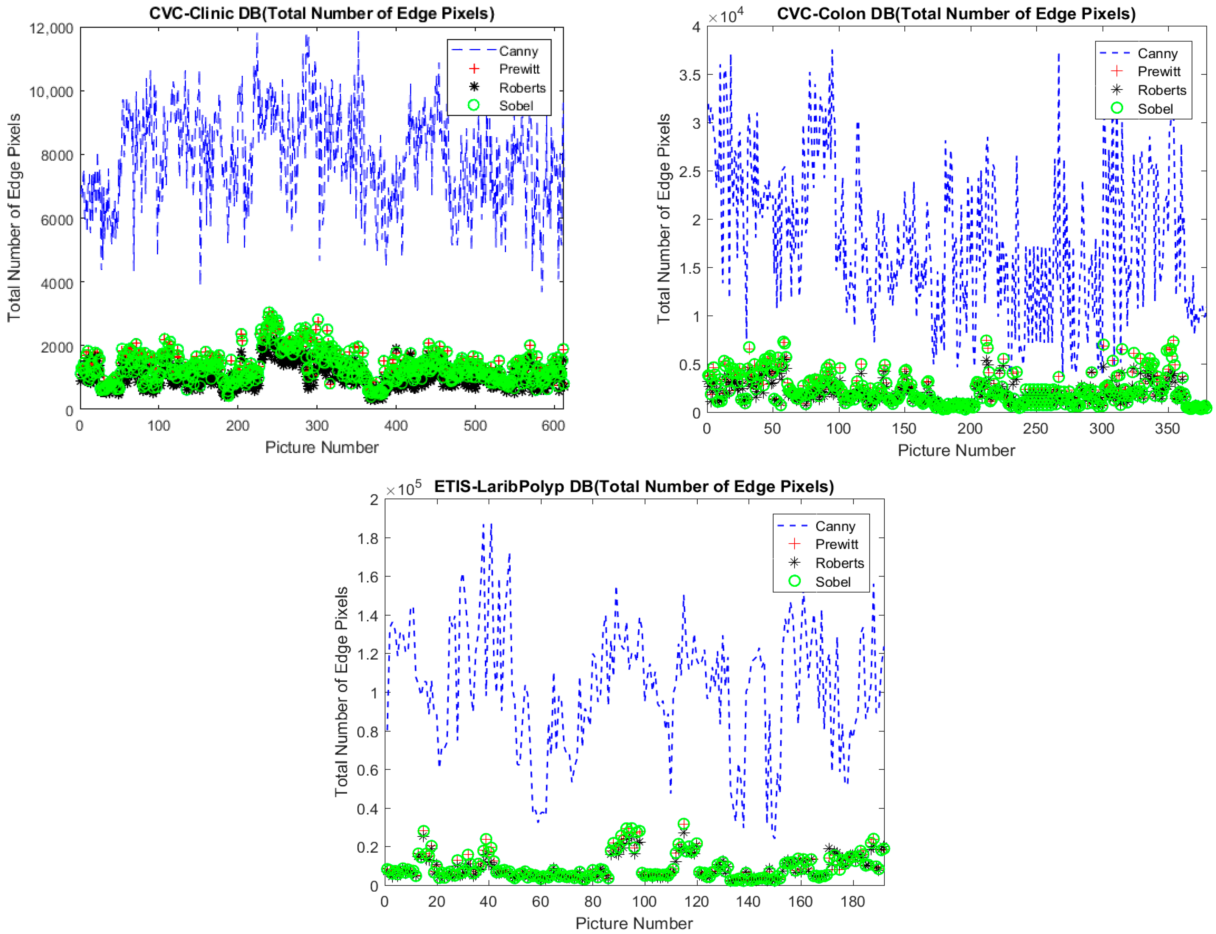
- Detecting polyp edges: Canny, Prewitt, Roberts, and Sobel techniques were applied as four different edge detection methods (Figure 5a,c,e,g respectively). By employing this edge detection operation, it becomes possible to decrease the time required for the following pre-processing steps and offers a comparatively consistent data source that tolerates geometric and environmental variations while performing the Hough transform calculations. The total number of edge pixels resulting from each filtering technique for all the images of the three databases was calculated and plotted in Figure 6.
- Finding the gradient-weighted edges: The edge filtered images (Figure 5a,c,e,g) were multiplied by the gradient magnitude output (Figure 4f). The reason for performing this multiplication step is to determine the gradient magnitude domain, where the polyp edges are most likely to be present within the whole gradient domain.As an example, we received images like (Figure 5b,d,f,h) for Canny, Prewitt, Roberts, and Sobel techniques. (It is visible, that in contrast with the full gradient subplot (Figure 4f), subplots (Figure 5b,d,f,h) contain the gradient values only where the edge mask value is 1, i.e., where the white pixels are located in subplots (Figure 5a,c,e,g).
- Normalizing: To make the proposed approach universally applicable, for all the pictures in all the databases, the gradient-weighted edges pixels were normalized into the interval [0, 1] for each image separately.
- Counting the number of the edge pixels located inside the ring mask, (this number serves as the reference: it is the number of the useful edge pixels).
- Calculating the final evaluation metrics: Considering our application requirements, two quantities were introduced to evaluate each of the four implemented edge detection methods. For each image of the three studied databases, the statistics calculated in the previous steps (the total number of pixels in the polyp mask contour, the total number of edge pixels resulted from each edge detection method, and the total number of edge pixels inside the ring mask) were used in composition the following two metrics.
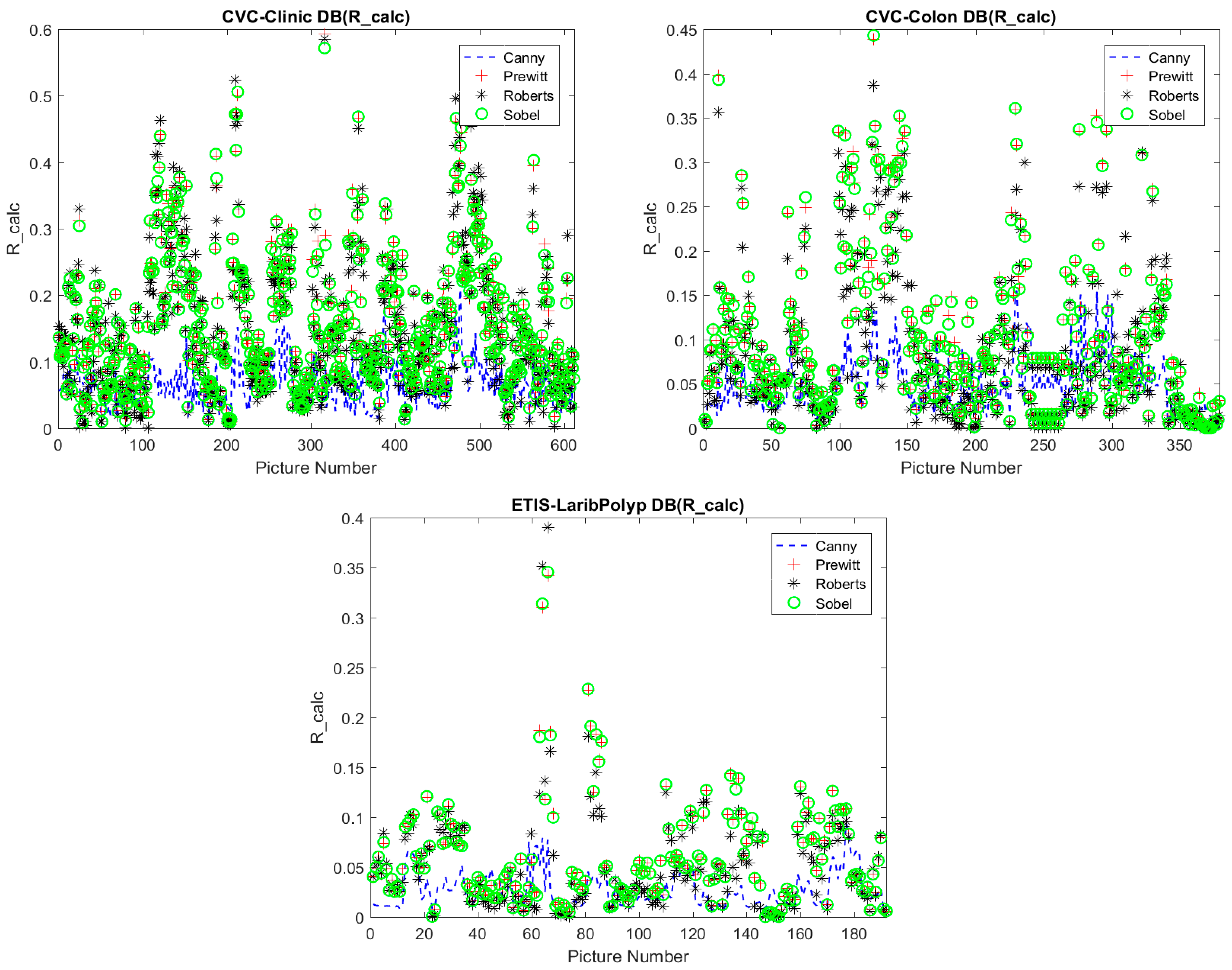
- The first evaluation parameter, i.e., the one referring to the calculation efficiency, is defined by the ratio between the number of edge pixels in the ring mask around the polyp contour and the total number of edge pixels in the entire image,This ratio represents the quality of the edge detection method with regard to the Hough transforms and polyp detection. values’ range is between 0 and 1. The higher this ratio is, the fewer non-mask contour edges are identified, and the less unneeded calculation is required in the classical or fuzzy Hough transform. Figure 7 shows the values of this metric resulting from Canny, Prewitt, Roberts, and Sobel filtering techniques for the three databases.
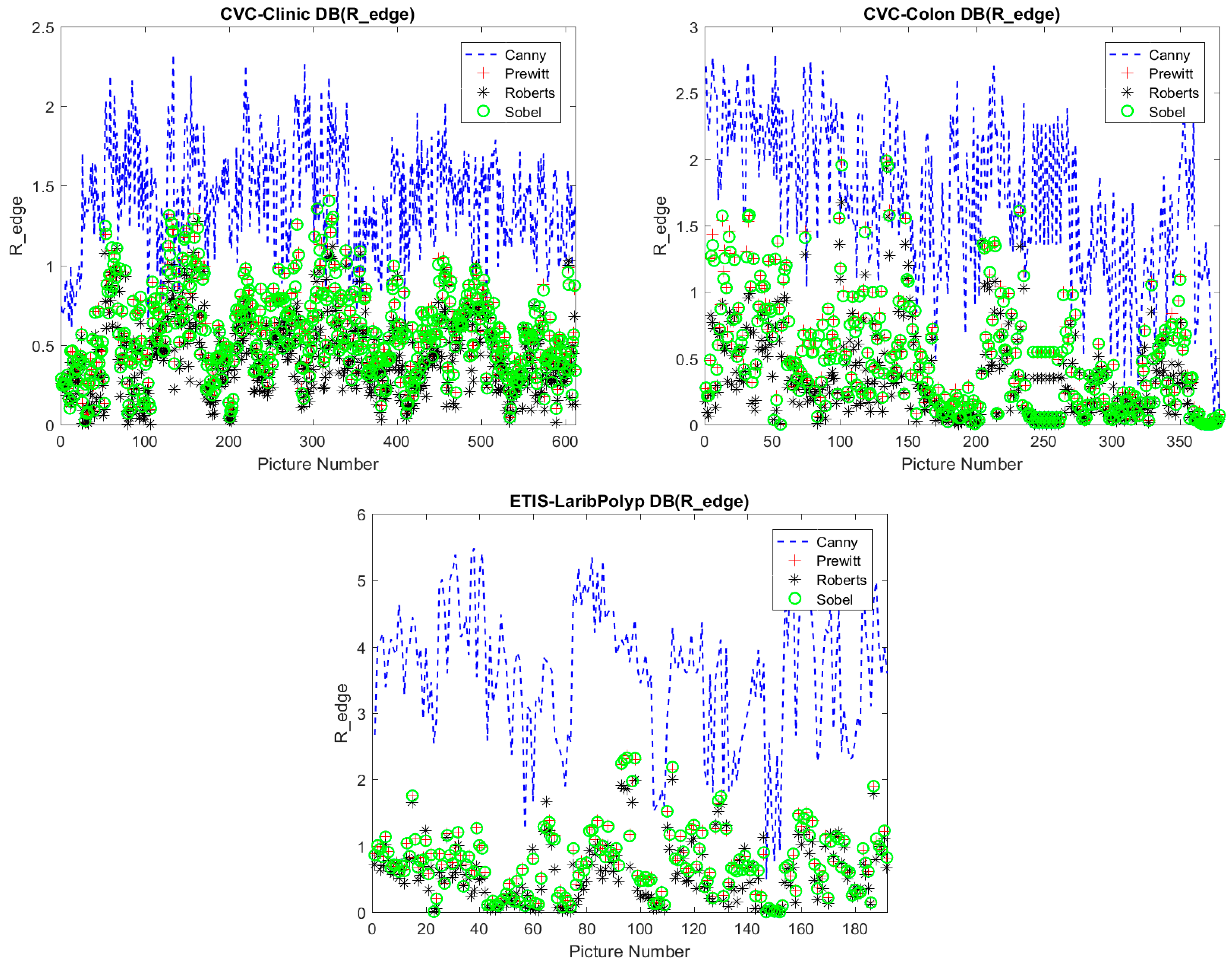
- The second evaluation parameter, i.e., the metric referring to the goodness of the edge pixels finding the ideal polyp contour (derived from the ground truth mask), is given by the ratio between the number of edge pixels in the ring mask and the number of pixels in the database polyp mask contour,In ideal case, this ratio should be as close to 1 as possible. Figure 8 displays the values of this metric resulting from all edge detection techniques for all studied databases.We have to note that the detected edge pixels in the ring mask may not exactly be the same as the edge pixels in the manually drawn database mask contour, but it still could be used for finding the polyp.
- Selecting the most appropriate edge detection technique: Canny method detects a wide range of fine edges and gives a dense detailed edges map. It also tends to connect edge pixels to continuous edge lines, in contrast with the other three techniques. Figure 6 clearly shows the large difference between the total number of edge pixels resulting from Canny and the other three edge detection methods. Prewitt, Roberts, and Sobel have very similar results for the majority of samples. As we are interested not only in decreasing the number of edge points scanned by the Hough transform, but also in increasing the efficiency of finding the colorectal polyp, we relied on the definition of the previous two evaluation metrics and as a basic for selecting the most appropriate edge detection technique as following.
- Selection of the most appropriate edge detection technique using : We tested two different selection strategies using metric . Based on the definition of , the nearest the value to 1 is, the better the filter is.According to the 1st strategy, we can select the filter, that has the mean of the metric values closest to 1. For each database and each type of the four edge detection methods we calculated the mean of the values.However, for the values of metric , in all databases, for all the four edge detection techniques, there was many samples between [0, 0.1], as it is visible in Figure 7. This is the reason why another strategy has to be considered as well.According to the 2nd strategy, we can select the filter, which has the most samples close to the ideal value. For this purpose, a goodness interval can be defined, and the number of samples within that interval can be calculated. In our case, for every edge detection technique, we checked how many samples in each database had a value greater than 0.1 as a measure of the filter suitability. Accordingly, the higher the number of resulting samples, the better the filter is. Of course, the percentage of this number within the total number of images in each database has to be considered; database CVC-Clinic [9] has 612 images, database CVC-Colon [42] has 379 images, and database ETIS-Larib [34] has 196 images). Table 2 lists the total results of this step.
- Selection of the most appropriate edge detection technique using : We also tested two different choosing strategies based on metric .According to the 1st strategy, similar to what we executed for , we can test how similar the results to their ideal value are. However, instead of calculating the mean value, we calculated the mean absolute error (MAE) value for metric from its ideal value 1. For this criterion, the smallest MAE value nominates the better filter.According to the 2nd strategy, as metric should be as close to 1 as possible, we suggested finding the goodness interval around , i.e., considering each sample that has value within [0.5, 1.5] among the good samples. Consequently, the higher the number of samples within the goodness interval, the better the filter is. Table 3 arranges the total results of this step.
3.2. Gradient-Based Thresholding for Prewitt Edge Detection Results
3.3. Gradient-Weighted Voting Approach for Classical and Fuzzy Hough Transforms
| Algorithm 3: Fuzzy Hough transform for a circle with parameters a, b, and r with gradient-weighted voting approach | |
| Requirements: an edge image with size a gradient magnitude image with size a finite parameter space with size , , with initial values of 0 a threshold for peak percentage , a threshold interval for the gradient magnitudes a voting membership matrix with size a result image , with size , with initial values of 0 | |
| 1: | for each image row from 1 to |
| 2: | for each image column from 1 to |
| 3: | for each parameter space row from 1 to |
| 4: | for each parameter space column from 1 to |
| 5: | for each parameter space 3rd dimension from 1 to |
| 6: | if and |
| 7: | … |
| 8: | end if |
| 9: | end for |
| 10: | end for |
| 11: | end for |
| 12: | end for |
| 13: | end for |
| 14: | compute the global maximum in |
| 15: | compute local maxima |
| 16: | select local maxima with |
| 17: | calculate the number of the local maxima from line 16 |
| 18: | for each local maximum from 1 to |
| 19: | for each result image row from 1 to |
| 20: | for each result image column from 1 to |
| 21: | if |
| 22: | |
| 23: | end if |
| 24: | end for |
| 25: | end for |
| 26: | end for |
4. Results and Discussion
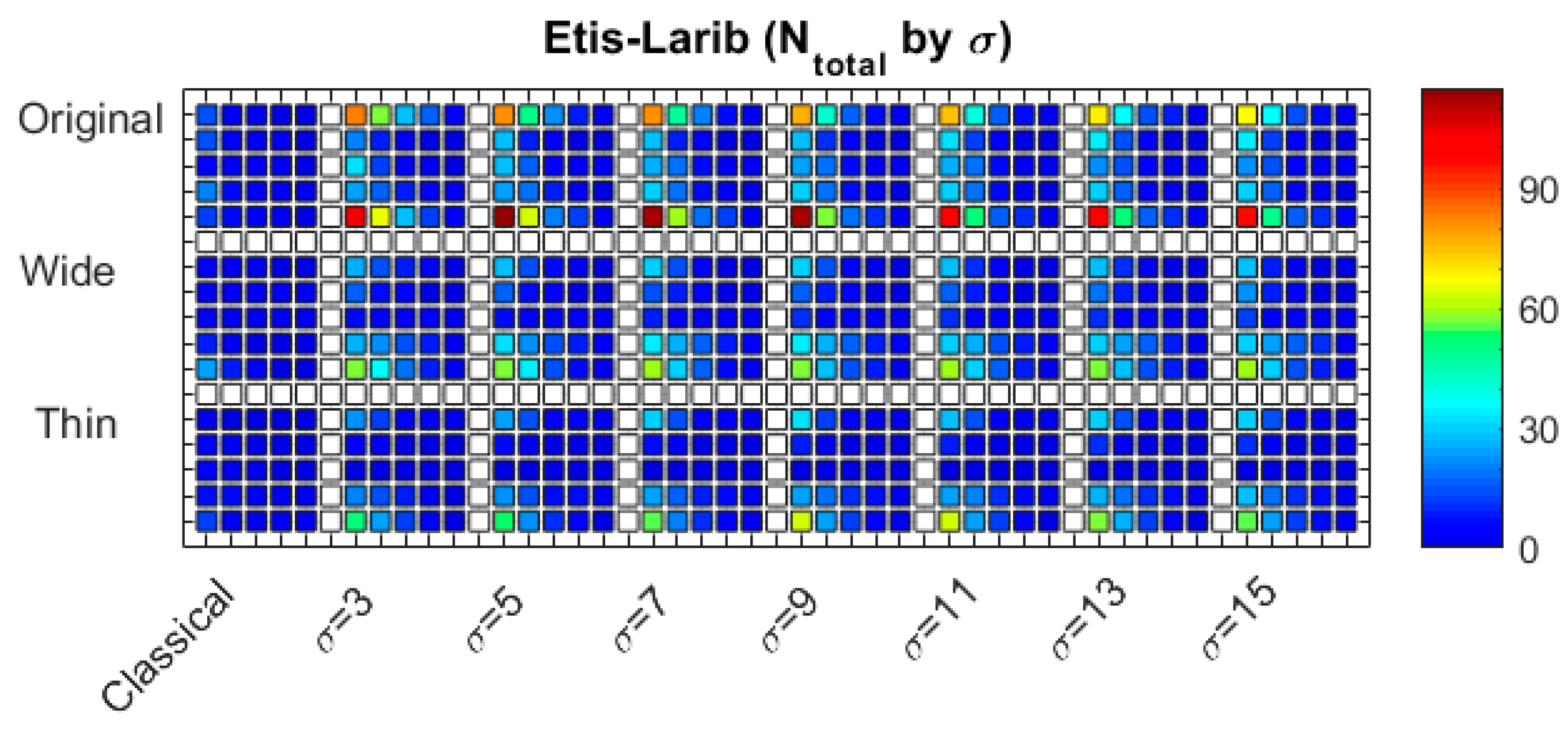
4.1. Number of Circles Found by the Algorithm
4.2. Roundness Metrics Evaluation
4.3. Time Evaluation
5. Conclusions
Author Contributions
Funding
Institutional Review Board Statement
Informed Consent Statement
Data Availability Statement
Conflicts of Interest
Appendix A


| (14) | A ratio to represent the quality of the edge detection method regarding the calculation efficiency of Hough transforms and polyp detection |
| (15) | A ratio to measure the goodness of the edge pixels finding the ideal polyp contour |
| and are the chosen values for the width of the voting membership function of the fuzzy Hough transforms | |
| and are the peak percentage values of the selected local maximum thresholds of the global maximum of the votes | |
| The total number of the final resulting circles | |
| The number of final circles within the ring mask | |
| (16) | A metric to measure the effectiveness of finding polyp-related final circles |
| The minimum and maximum coordinates of the ground truth mask points in direction | |
| The minimum and maximum coordinates of the ground truth mask points in direction | |
| (17) | Average radius of the polyp mask |
| The and coordinates of the left of the polyp mask | |
| The radial displacement of mask contour point | |
| The maximum of the roundness error | |
| Original | The full Hough transforms for all the edge points |
| Wide | The restricted Hough transforms for the edge points with normalized gradient values within a wide threshold interval [0.06, 0.3] |
| Thin | The restricted Hough transforms for the edge points with normalized gradient values within a thin threshold interval [0.08, 0.2] |
References
- Alam, M.J.; Fattah, S.A. SR-AttNet: An Interpretable Stretch-Relax Attention based Deep Neural Network for Polyp Segmentation in Colonoscopy Images. Comput. Biol. Med. 2023, 160, 106945. [Google Scholar] [CrossRef]
- Krenzer, A.; Banck, M.; Makowski, K.; Hekalo, A.; Fitting, D.; Troya, J.; Sudarevic, B.; Zoller, W.G.; Hann, A.; Puppe, F. A Real-Time Polyp Detection System with Clinical Application in Colonoscopy Using Deep Convolutional Neural Networks. J. Imaging 2023, 9, 26. [Google Scholar] [CrossRef]
- Yue, G.; Han, W.; Li, S.; Zhou, T.; Lv, J.; Wang, T. Automated polyp segmentation in colonoscopy images via deep network with lesion-aware feature selection and refinement. Biomed. Signal Process. Control 2022, 78, 103846. [Google Scholar] [CrossRef]
- Ahmad, O.F.; Brandao, P.; Sami, S.S.; Mazomenos, E.; Rau, A.; Haidry, R.; Vega, R.; Seward, E.; Vercauteren, T.K.; Stoyanov, D.; et al. Artificial intelligence for real-time polyp localization in colonoscopy withdrawal videos. Gastrointest. Endosc. 2019, 89, AB647. [Google Scholar] [CrossRef]
- Sornapudi, S.; Meng, F.; Yi, S. Region-based automated localization of colonoscopy and wireless capsule endoscopy polyps. Appl. Sci. 2019, 9, 2404. [Google Scholar] [CrossRef] [Green Version]
- Wittenberg, T.; Zobel, P.; Rathke, M.; Mühldorfer, S. Computer aided detection of polyps in whitelight-colonoscopy images using deep neural networks. Curr. Dir. Biomed. Eng. 2019, 5, 231–234. [Google Scholar] [CrossRef]
- Aliyi, S.; Dese, K.; Raj, H. Detection of gastrointestinal tract disorders using deep learning methods from colonoscopy images and videos. Sci. Afr. 2023, 20, e01628. [Google Scholar] [CrossRef]
- Karaman, A.; Pacal, I.; Basturk, A.; Akay, B.; Nalbantoglu, U.; Coskun, S.; Sahin, O.; Karaboga, D. Robust real-time polyp detection system design based on YOLO algorithms by optimizing activation functions and hyper-parameters with Artificial Bee Colony (ABC). Expert Syst. Appl. 2023, 221, 119741. [Google Scholar] [CrossRef]
- Bernal, J.; Sánchez, F.J.; Fernández-Esparrach, G.; Gil, D.; Rodríguez, C.; Vilariño, F. WM-DOVA maps for accurate polyp highlighting in colonoscopy: Validation vs. saliency maps from physicians. Comput. Med. Imaging Graph. 2015, 43, 99–111. [Google Scholar] [CrossRef]
- Iwahori, Y.; Hattori, A.; Adachi, Y.; Bhuyan, M.; Woodham, R.J.; Kasugai, K. Automatic Detection of Polyp Using Hessian Filter and HOG Features. Procedia Comput. Sci. 2015, 60, 730–739. [Google Scholar] [CrossRef] [Green Version]
- Rácz, I.; Horváth, A.; Szalai, M.; Spindler, S.; Kiss, G.; Regöczi, H.; Horváth, Z. Digital Image Processing Software for Predicting the Histology of Small Colorectal Polyps by Using Narrow-Band Imaging Magnifying Colonoscopy. Gastrointest. Endosc. 2015, 81, AB259. [Google Scholar] [CrossRef]
- Georgieva, V.; Nagy, S.; Kamenova, E.; Horváth, A. An Approach for Pit Pattern Recognition in Colonoscopy Images. Egypt. Comput. Sci. J. 2015, 39, 72–82. [Google Scholar]
- Hough, P.V.C. Machine Analysis of Bubble Chamber Pictures. In Proceedings of the 2nd International Conference on High-Energy Accelerators and Instrumentation, HEACC 1959, CERN, Geneva, Switzerland, 14–19 September 1959. [Google Scholar]
- Ballard, D.H. Generalizing the Hough Transform to detect arbitrary shapes. Pattern Recognit. 1981, 13, 111–122. [Google Scholar] [CrossRef] [Green Version]
- Nahum, K.; Eldar, Y.; Bruckstein, A.M. A probabilistic Hough Transform. Pattern Recognit. 1991, 24, 303–316. [Google Scholar] [CrossRef]
- Lei, X.; Erkki, O. Randomized Hough Transform (RHT): Basic Mechanisms, Algorithms, and Computational Complexities. CVGIP Image Underst. 1993, 57, 131–154. [Google Scholar] [CrossRef]
- Cucchiara, R.; Filicori, F. The Vector-Gradient Hough Transform. IEEE Trans. Pattern Anal. Mach. Intell. 1998, 20, 746–750. [Google Scholar] [CrossRef]
- Han, J.H.; Kóczy, L.T.; Poston, T. Fuzzy Hough Transform. Pattern Recognit. Lett. 1994, 15, 649–658. [Google Scholar] [CrossRef]
- Zhao, K.; Han, Q.; Zhang, C.; Xu, J.; Cheng, M. Deep Hough Transform for Semantic Line Detection. IEEE Trans. Pattern Anal. Mach. Intell. 2022, 44, 4793–4806. [Google Scholar] [CrossRef] [PubMed]
- Lin, G.; Tang, Y.; Zou, X.; Cheng, J.; Xiong, J. Fruit detection in natural environment using partial shape matching and probabilistic Hough transform. Precis. Agric 2020, 21, 160–177. [Google Scholar] [CrossRef]
- Liu, W.; Zhang, Z.; Li, S.; Tao, D. Road Detection by Using a Generalized Hough Transform. Remote Sens. 2017, 9, 590. [Google Scholar] [CrossRef] [Green Version]
- Mathavan, S.; Vaheesan, K.; Kumar, A.; Chandrakumar, C.; Kamal, K.; Rahman, M.; Stonecliffe-Jones, M. Detection of pavement cracks using tiled fuzzy Hough Transform. J. Electron. Imaging 2017, 26, 053008. [Google Scholar] [CrossRef] [Green Version]
- Pugin, E.; Zhiznyakov, A.; Zakharov, A. Pipes Localization Method Based on Fuzzy Hough Transform. In Advances in Intelligent Systems and Computing, Proceedings of the Second International Scientific Conference “Intelligent Information Technologies for Industry” (IITI’17); Abraham, A., Kovalev, S., Tarassov, V., Snasel, V., Vasileva, M., Sukhanov, A., Eds.; IITI 2017; Springer: Cham, Switzerland, 2018; Volume 679, pp. 536–544. [Google Scholar] [CrossRef]
- Nagy, S.; Solecki, L.; Sziová, B.; Sarkadi-Nagy, B.; Kóczy, L.T. Applying Fuzzy Hough Transform for Identifying Honed Microgeometrical Surfaces. In Computational Intelligence and Mathematics for Tackling Complex Problems; Kóczy, L., Medina-Moreno, J., Ramírez-Poussa, E., Šostak, A., Eds.; Studies in Computational Intelligence; Springer: Cham, Switzerland, 2020; Volume 819, pp. 35–42. [Google Scholar] [CrossRef]
- Nagy, S.; Kovács, M.; Sziová, B.; Kóczy, L.T. Fuzzy Hough Transformation in aiding computer tomography-based liver diagnosis. In Proceedings of the 2019 IEEE AFRICON, Accra, Ghana, 15–17 September 2019. [Google Scholar] [CrossRef]
- Djekoune, A.; Messaoudi, K.; Amara, K. Incremental circle hough transform: An improved method for circle detection. Optik 2017, 133, 17–31. [Google Scholar] [CrossRef]
- Hapsari, R.K.; Utoyo, M.I.; Rulaningtyas, R.; Suprajitno, H. Iris segmentation using Hough Transform method and Fuzzy C-Means method. J. Phys. Conf. Ser. 2020, 1477, 022–037. [Google Scholar] [CrossRef]
- Vijayarajeswari, R.; Parthasarathy, P.; Vivekanandan, S.; Basha, A.A. Classification of mammogram for early detection of breast cancer using SVM classifier and Hough transform. Measurement 2019, 146, 800–805. [Google Scholar] [CrossRef]
- Shaaf, Z.F.; Jamil, M.M.A.; Ambar, R. Automatic Localization of the Left Ventricle from Short-Axis MR Images Using Circular Hough Transform. In Lecture Notes in Networks and Systems, Proceedings of the Third International Conference on Trends in Computational and Cognitive Engineering; Kaiser, M.S., Ray, K., Bandyopadhyay, A., Jacob, K., Long, K.S., Eds.; Springer: Singapore, 2022; Volume 348, p. 348. [Google Scholar] [CrossRef]
- Chen, J.; Qiang, H.; Wu, J.; Xu, G.; Wang, Z. Navigation path extraction for greenhouse cucumber-picking robots using the prediction-point Hough transform. Comput. Electron. Agric. 2021, 180, 105911. [Google Scholar] [CrossRef]
- Chuquimia, O.; Pinna, A.; Dray, X.; Granado, B. A Low Power and Real-Time Architecture for Hough Transform Processing Integration in a Full HD-Wireless Capsule Endoscopy. IEEE Trans. Biomed. Circuits Syst. 2020, 14, 646–657. [Google Scholar] [CrossRef]
- Montseny, E.; Sobrevilla, P.; Marès Martí, P. Edge orientation-based fuzzy Hough transform (EOFHT). In Proceedings of the 3rd Conference of the European Society for Fuzzy Logic and Technology, Zittau, Germany, 10–12 September 2003. [Google Scholar]
- Barbosa, W.O.; Vieira, A.W. On the Improvement of Multiple Circles Detection from Images using Hough Transform. TEMA 2019, 20, 331–342. [Google Scholar] [CrossRef]
- Silva, J.; Histace, A.; Romain, O.; Dray, X.; Granado, B. Toward embedded detection of polyps in WCE images for early diagnosis of colorectal cancer. Int. J. Comput. Assist. Radiol. Surg. 2014, 9, 283–293. [Google Scholar] [CrossRef] [PubMed]
- Ruano, J.; Barrera, C.; Bravo, D.; Gomez, M.; Romero, E. Localization of Small Neoplastic Lesions in Colonoscopy by Estimating Edge, Texture and Motion Saliency. In Proceedings of the Annual International Conference of the IEEE Engineering in Medicine and Biology Society, Berlin, Germany, 23–27 July 2019; pp. 5945–5948. [Google Scholar] [CrossRef]
- Ruiz, L.; Guayacán, L.; Martínez, F. Automatic polyp detection from a regional appearance model and a robust dense Hough coding. In Proceedings of the 2019 XXII Symposium on Image, Signal Processing and Artificial Vision (STSIVA), Bucaramanga, Colombia, 24–26 April 2019; pp. 1–5. [Google Scholar] [CrossRef]
- Yao, H.; Stidham, R.W.; Soroushmehr, R.; Gryak, J.; Najarian, K. Automated Detection of Non-Informative Frames for Colonoscopy Through a Combination of Deep Learning and Feature Extraction. In Proceedings of the Annual International Conference of the IEEE Engineering in Medicine and Biology Society, Berlin, Germany, 23–27 July 2019; pp. 2402–2406. [Google Scholar] [CrossRef]
- Ismail, R.; Nagy, S. On Metrics Used in Colonoscopy Image Processing for Detection of Colorectal Polyps. In New Approaches for Multidimensional Signal Processing; Kountchev, R., Mironov, R., Li, S., Eds.; Smart Innovation, Systems and Technologies; Springer: Singapore, 2021; Volume 216, pp. 137–151. [Google Scholar] [CrossRef]
- Ismail, R.; Nagy, S. Ways of improving of active contour methods in colonoscopy image segmentation. Image Anal. Stereol. 2022, 41, 7–23. [Google Scholar] [CrossRef]
- Nagy, S.; Ismail, R.; Sziová, B.; Kóczy, L.T. On classical and fuzzy Hough transform in colonoscopy image processing. In Proceedings of the IEEE AFRICON 2021, Virtual Conference, Arusha, Tanzania, 13–15 September 2021; pp. 124–129. [Google Scholar] [CrossRef]
- Ismail, R.; Prukner, P.; Nagy, S. On Applying Gradient Based Thresholding on the Canny Edge Detection Results to Improve the Effectiveness of Fuzzy Hough Transform for Colonoscopy Polyp Detection Purposes. In New Approaches for Multidimensional Signal Processing; Kountchev, R., Mironov, R., Nakamatsu, K., Eds.; NAMSP 2022. Smart Innovation, Systems and Technologies; Springer: Singapore, 2023; Volume 332, pp. 110–121. [Google Scholar] [CrossRef]
- Bernal, J.; Sanchez, F.J.; Vilariño, F. Towards Automatic Polyp Detection with a Polyp Appearance Model. Pattern Recognit. 2012, 45, 3166–3182. [Google Scholar] [CrossRef]
- Zadeh, L.A. Fuzzy Sets. Inf. Control 1965, 8, 338–353. [Google Scholar] [CrossRef] [Green Version]
- Roberts, L. Machine Perception of 3-D Solids. Ph.D. Thesis, Massachusetts Institute of Technology, Department of Electrical Engineering, Cambridge, MA, USA, 1965. [Google Scholar]
- Prewitt, J.M.S. Object enhancement and extraction. In Picture Processing and Psychopictorics, 1st ed.; Lipkin, B., Rosenfeld, A., Eds.; Academic Press: New York, NY, USA, 1970; pp. 75–149. [Google Scholar]
- Sobel, I. Neighborhood coding of binary images for fast contour following and general binary array processing. Comput. Graph. Image Process. 1978, 8, 127–135. [Google Scholar] [CrossRef]
- Canny, J. A computational approach to edge detection. IEEE Trans. Pattern Anal. Mach. Intell. 1986, 8, 679–698. [Google Scholar] [CrossRef]
- Kalbasi, M.; Nikmehr, H. Noise-Robust, Reconfigurable Canny Edge Detection and its Hardware Realization. IEEE Access 2020, 8, 39934–39945. [Google Scholar] [CrossRef]
- Csimadia, G.; Nagy, S. The Effect of the Contrast Enhancement Processes on the Structural Entropy of Colonoscopic Images. In Proceedings of the ICEST 2014, Nis, Serbia, 20–27 June 2014. [Google Scholar]
- Pogorelov, K.; Randel, K.R.; Griwodz, C.; Eskeland, S.L.; de Lange, T.; Johansen, D.; Spampinato, C.; Dang-Nguyen, D.-T.; Lux, M.; Schmidt, P.T.; et al. KVASIR: A Multi-Class Image Dataset for Computer Aided Gastrointestinal Disease Detection. In Proceedings of the 8th ACM on Multimedia Systems Conference 2017, Taipei, Taiwan, 20–23 June 2017; pp. 164–169. [Google Scholar] [CrossRef] [Green Version]


| Strengths | Weaknesses |
|---|---|
|
|
|
|
|
|
| |
|
|
|
| Canny | Prewitt | Roberts | Sobel | ||
|---|---|---|---|---|---|
| 1st strategy: Mean | 0.063001 | 0.153718 | 0.147087 | 0.152823 | CVC-Clinic |
| 0.04806 | 0.099965 | 0.081437 | 0.09925 | CVC-Colon | |
| 0.026186 | 0.06001 | 0.049776 | 0.059926 | ETIS-Larib | |
| 2nd strategy: Num. of samples with | 70 | 394 | 360 | 394 | CVC-Clinic |
| 29 | 138 | 108 | 141 | CVC-Colon | |
| 0 | 35 | 22 | 33 | ETIS-Larib |
| Canny | Prewitt | Roberts | Sobel | ||
|---|---|---|---|---|---|
| 1st strategy: MAE | 0.459919 | 0.447193 | 0.579451 | 0.44937 | CVC-Clinic |
| 0.779827 | 0.582246 | 0.683746 | 0.588328 | CVC-Colon | |
| 2.609909 | 0.44718 | 0.536933 | 0.451125 | ETIS-Larib | |
| 2nd strategy: Num. of samples with | 346 | 353 | 221 | 349 | CVC-Clinic |
| 132 | 156 | 90 | 152 | CVC-Colon | |
| 4 | 122 | 88 | 121 | ETIS-Larib |
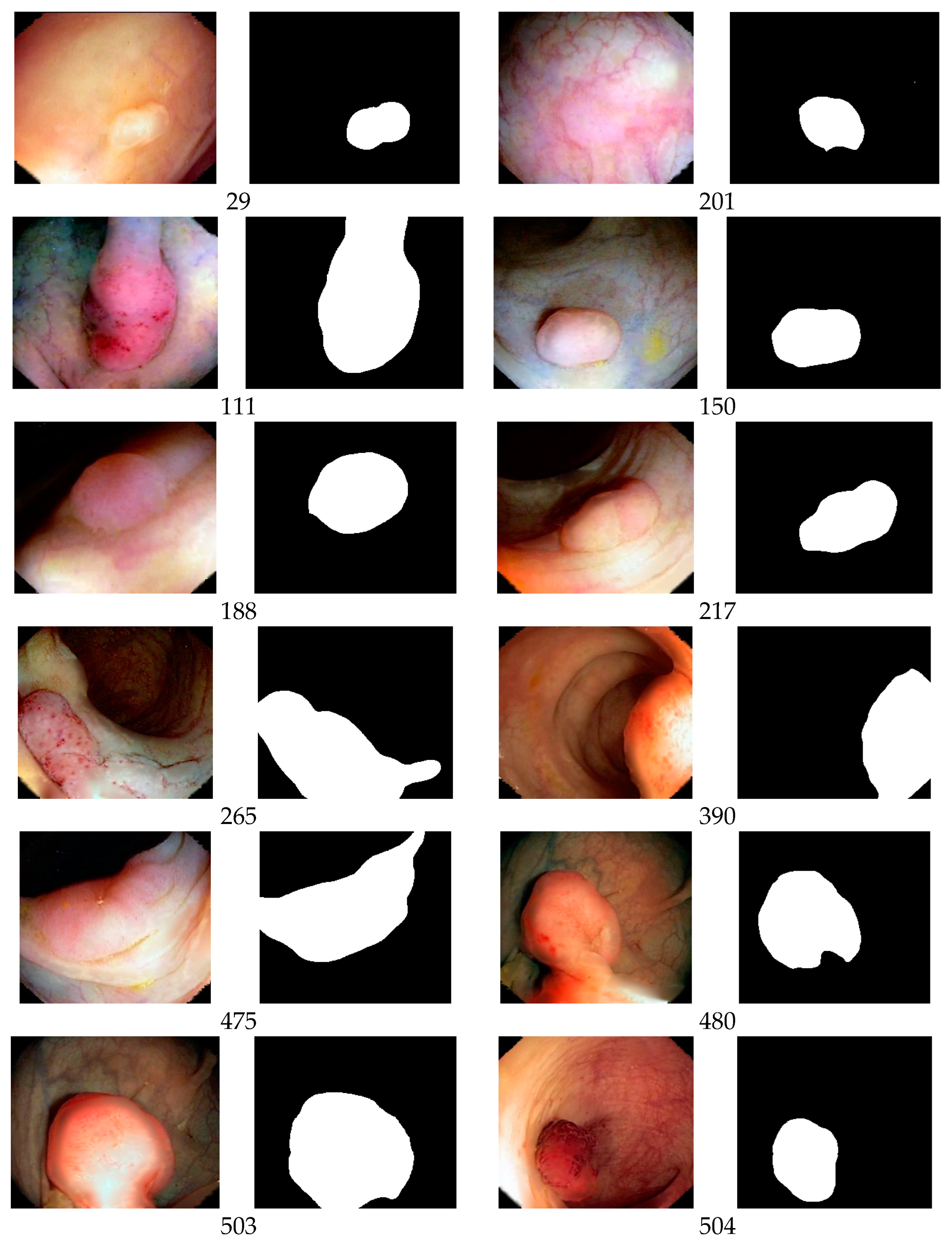
| Database | Image | No. of Edge Pixels | ||||
|---|---|---|---|---|---|---|
| CVC-Clinic | 29 | 0.004918033 | 0.013274336 | 610 | 38.75 | 0.358 |
| 201 | 0.008460237 | 0.038314176 | 1182 | 68 | 0.957 | |
| 111 | 0.247629671 | 0.733884298 | 1793 | 92.75 | 0.380 | |
| 150 | 0.251902588 | 1.054140127 | 1314 | 52 | 0.261 | |
| 188 | 0.364678899 | 0.424 | 436 | 66.5 | 0.173 | |
| 217 | 0.230191827 | 0.74393531 | 1199 | 64.5 | 0.409 | |
| 265 | 0.260652765 | 0.871212121 | 2206 | 110 | 0.775 | |
| 390 | 0.297808765 | 0.641630901 | 1004 | 75.75 | 0.366 | |
| 475 | 0.367805755 | 0.653354633 | 1112 | 106.5 | 0.757 | |
| 480 | 0.222554145 | 0.685057471 | 1339 | 72.75 | 0.315 | |
| 503 | 0.310214376 | 0.976190476 | 1586 | 84.75 | 0.151 | |
| 504 | 0.180173092 | 0.68358209 | 1271 | 56.75 | 0.201 | |
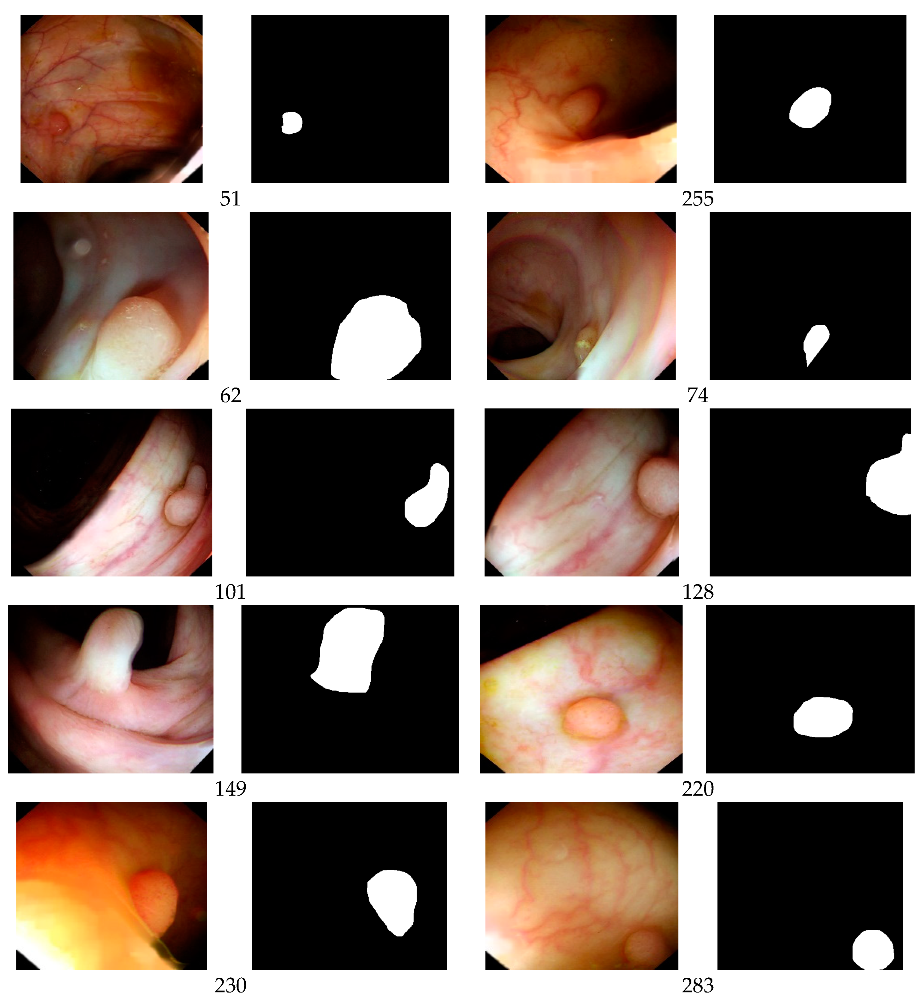
| CVC-Colon | 51 | 0.004398827 | 0.035087719 | 1364 | 27 | 0.278 |
| 255 | 0.002773925 | 0.006779661 | 721 | 52.25 | 0.299 | |
| 62 | 0.242270224 | 0.801120448 | 2361 | 117 | 0.337 | |
| 74 | 0.218066743 | 1.457692308 | 1738 | 46.25 | 0.694 | |
| 101 | 0.180649379 | 1.978520286 | 4589 | 71.5 | 0.711 | |
| 128 | 0.182273052 | 0.44973545 | 1399 | 84 | 0.483 | |
| 149 | 0.215956424 | 1.099510604 | 3121 | 98 | 0.334 | |
| 220 | 0.149488927 | 0.966942149 | 2348 | 59.5 | 0.202 | |
| 230 | 0.318594104 | 0.641552511 | 882 | 74.25 | 0.442 | |
| 283 | 0.194486983 | 0.404458599 | 653 | 52.25 | 0.132 | |
| ETIS-Larib | 24 | 0.007230077 | 0.204545455 | 6224 | 39.75 | 0.135 |
| 151 | 0.0010755 | 0.012437811 | 4649 | 70.75 | 0.507 | |
| 25 | 0.104344123 | 0.879186603 | 7044 | 153.25 | 0.549 | |
| 65 | 0.117593198 | 1.24 | 7645 | 125.25 | 0.249 | |
| 82 | 0.191721133 | 1.269230769 | 4131 | 113.25 | 0.321 | |
| 138 | 0.102428256 | 0.649859944 | 2265 | 63.5 | 0.449 | |
| 160 | 0.129833607 | 1.297423888 | 8534 | 151 | 0.430 |
| Artificial Image | Axes (Pixels) | |||
|---|---|---|---|---|
 | 30, 30 | 15.5 | 0.6508 | 0.042 |
| 30, 25 | 14 | 1.8902 | 0.135 | |
| 30, 20 | 13 | 2.8758 | 0.221 | |
| 30, 15 | 11.75 | 4.7322 | 0.403 | |
| 30, 10 | 10.5 | 5.0081 | 0.477 | |
 | 60, 60 | 30.5 | 0.7931 | 0.026 |
| 60, 50 | 28 | 2.8902 | 0.103 | |
| 60, 40 | 25.5 | 5.2002 | 0.204 | |
| 60, 30 | 23 | 7.6023 | 0.331 | |
| 60, 20 | 20.5 | 10.0369 | 0.490 | |
 | 90, 90 | 45.5 | 1.6081 | 0.035 |
| 90, 75 | 41.5 | 4.2220 | 0.102 | |
| 90, 60 | 38 | 8.4958 | 0.224 | |
| 90, 45 | 34.25 | 12.1989 | 0.356 | |
| 90, 30 | 30.5 | 15.0686 | 0.494 |
Disclaimer/Publisher’s Note: The statements, opinions and data contained in all publications are solely those of the individual author(s) and contributor(s) and not of MDPI and/or the editor(s). MDPI and/or the editor(s) disclaim responsibility for any injury to people or property resulting from any ideas, methods, instructions or products referred to in the content. |
© 2023 by the authors. Licensee MDPI, Basel, Switzerland. This article is an open access article distributed under the terms and conditions of the Creative Commons Attribution (CC BY) license (https://creativecommons.org/licenses/by/4.0/).
Share and Cite
Ismail, R.; Nagy, S. A Novel Gradient-Weighted Voting Approach for Classical and Fuzzy Circular Hough Transforms and Their Application in Medical Image Analysis—Case Study: Colonoscopy. Appl. Sci. 2023, 13, 9066. https://doi.org/10.3390/app13169066
Ismail R, Nagy S. A Novel Gradient-Weighted Voting Approach for Classical and Fuzzy Circular Hough Transforms and Their Application in Medical Image Analysis—Case Study: Colonoscopy. Applied Sciences. 2023; 13(16):9066. https://doi.org/10.3390/app13169066
Chicago/Turabian StyleIsmail, Raneem, and Szilvia Nagy. 2023. "A Novel Gradient-Weighted Voting Approach for Classical and Fuzzy Circular Hough Transforms and Their Application in Medical Image Analysis—Case Study: Colonoscopy" Applied Sciences 13, no. 16: 9066. https://doi.org/10.3390/app13169066