Comparison of Mixing Plane, Frozen Rotor, and Sliding Mesh Methods on a Counter-Rotating Dual-Rotor Wind Turbine

Abstract

Nowadays, there are numerous new features available in CFD (computational fluid dynamics) that can simulate complex physical phenomena, which used to be challenging to address. However, in current CFD software, certain problems can be simulated using different approaches. In our article, we chose different rotating motion methods to analyze a counter-rotating dual-rotor wind turbine (CO-DRWT). Using the different rotating motion approaches we selected (mixing plane, frozen rotor, and sliding mesh), we examined the torque on the rotors and compared them. The following conclusion was reached. If transient fluid flow must be examined, then the sliding mesh method provided the most realistic results, while the frozen rotor method was adequate if we investigated the effect of wake and vortex near the rotating blades or on its environment. The mixing plane method should be used when the focus is on the kinetics and kinematics of the rotating blade or structure.

1. Introduction

Nowadays, numerical simulations are more often used compared to experiments with a physically built prototype. Depending on the requested output, the results of virtual testing can be different. Some of these methods include computational fluid dynamics (CFD), finite element analysis (FEA), and multibody dynamics simulations (MBDSs). CFD software provides more and more features year by year. Their solvers are optimized for fast and efficient running on a local PC or an HPC (high-performance computing) cloud computing server [1].

CFD is an excellent tool that allows us to model and simulate how engineering devices behave in practice. With a certain accuracy, it is possible to estimate their performance based on the obtained numerical data from simulations [2,3]. In our article, we focus only on rotating motion modeling by using an unconventional wind turbine (WT). It must be mentioned that the compressibility effect was neglected; therefore, we did not include the energy equation in our model.

Due to the increasing energy demand, clean and renewable energy sources are becoming very popular sources. The current energy mix contains more oil, coal–gas, and coal-fired and nuclear sources such as wind, solar, hydropower, bioenergy, and geothermal sources. By 2025, the energy demand will grow to 62 PWh/year, and it will contain more wind and solar than the other previously mentioned sources [4,5,6].

Among renewable energies, wind energy is a rapidly growing sector. This growth is achievable with traditional WTs, but it is more feasible with unconventional ones [7,8,9,10].

Unconventional WTs are special types of wind turbines that have been modified to meet specific requirements, e.g., installation territory.

In Figure 1a, we can see a counter-rotating dual-rotor wind turbine (CO-DRWT) that has two rotors; thus, it can achieve a higher power coefficient (c_p) and generate more electrical energy than a single-rotor wind turbine (SRWT) [8,9]. In Figure 1b, there is an augmented WT with a baffle to catch more wind, while in Figure 1c, the Archimedes screw WT is presented, which operates at a low noise level, and is suitable for urban areas [11,12,13].

The main goal of our article is to compare different rotary motion modeling methods in CFD applied on CO-DRWT and to demonstrate the advantages and disadvantages of the applied methods.

2. Foundation of CFD

Computational fluid dynamics (CFD) is a tool used to model and simulate fluid and thermal behaviors numerically. CFD predicts continuum behaviors using different methods, such as the finite volume method (FVM), finite difference method (FDM), or smoothed particle hydrodynamics (SPH). Each method is based on a certain type of discretization. In our research, we use FVM, which divides the computational domain into finite volumes, which is known in practice as a mesh or grid. For these mesh elements, the CFD solver creates a discrete equation system based on the following transport equation:

$$\frac{\partial }{\partial t}{{\displaystyle \int }}_V^{}\rho \varphi dV+{{\displaystyle \oint }}_A^{}\rho \varphi VdA-{{\displaystyle \int }}_V^{}{S}_{\varphi }dA-{{\displaystyle \oint }}_A^{}\mathsf{\Gamma }\nabla \varphi dA=R$$

(1)

In this equation, V denotes an arbitrary enclosed control volume, A denotes the surface of this control volume, ρϕ is the conserved quantity (e.g., mass), F is the same quantity’s flux over the A surface, S_ϕ is the volumetric source of quantity, ρϕ (potential energy) over volume V, Γ$\nabla$ϕ is the surface source of quantity, ρϕ over surface A, and R is the error of the equation (residual) [17].

From Equation (1), the mass and the momentum equation can be derived. In a Cartesian coordinate system, these laws can be described using the following equations:

$$\frac{\partial \rho }{\partial t}+\frac{\partial }{\partial x_i}\left(\rho u_i\right)=0$$

(2)

$$\frac{\partial \rho u_i}{\partial t}+\frac{\partial }{\partial x_j}\left(\rho u_i{u}_j\right)+\frac{\partial p}{\partial x_i}=\frac{\partial }{\partial x_j}\left({\tau }_{ij}+{\tau }_{ij}^R\right)+S_i$$

(3)

In Equations (2) and (3), i and j indexes are the directions in the Cartesian coordinate system, while their values are i = 1, 2, 3 and j = 1, 2, 3, u is the fluid velocity, $\rho$ is the fluid density, $S_i$ is a mass-distributed external force per unit mass, which contains the gravity ($S_i^{gravity}$), the coordinate system’s rotation ($S_i^{rotation})$, and the other external forces ($S_i=S_i^{rotation}+S_i^{rotation}+\dots )$, ${\tau }_{ij}$ is the viscous shear stress tensor, while t denotes time.

Using the i and j subscripts, we can define velocities and special directions in a three-dimensional space, e.g., the velocity vector would equal as follows:

$$u=u_x·e_x+u_y·e_y+u_z·e_z$$

(4)

if we use the x, y, and z directions instead of the 1, 2, and 3.

In a rotating reference frame, the external force from the rotation can be written as follows:

$$S_i^{rotation}=-2e_{ijk}{\mathsf{\Omega }}_j\rho u_k+\rho {\mathsf{\Omega }}^2{r}_i$$

(5)

where ${ϵ}_{ijk}$ is the Levy-Civita symbol, $\mathsf{\Omega }$ is the angular velocity, and r is the vector pointing to the axis of rotation.

If heat transfer and/or compressibility is modeled, then conservation law is used in the modeling. However, compressibility and heat effect were not in the scope of our aims; therefore, we did not include the energy equation in our model. It must be mentioned that this study sets the focus on traditional, second-order schemes, which are available in commercial CFD software (Simcenter STAR CCM+, V2022.1), although there are higher-order schemes [18,19] as well.

3. Methods for Modeling and Simulating Rotational Motion

There are several approaches to modeling rotating motion in CFD, for example, mixing plane, frozen rotor, sliding mesh, morphing mesh, or the overset mesh method. Each method has its own advantages and disadvantages. In this current paper, we used mixing plane, frozen rotor, and sliding mesh approaches, which shall be introduced briefly in the following paragraphs.

The mixing plane interface is also known as stage or averaged rotating local region in some CFD software [20]. With the mixing plane method, the interaction between two regions can be simulated, in which one of them is a stator, or a nonrotating region, while the other one is a rotor, which carries out the actual rotation.

This method can model and simulate steady and unsteady flows. When this approach is used in the rotating region, the governing equation is solved in a rotating coordinate system, while in the stationery region, the equations are solved in a stationary coordinate system. Within the rotating region, the flow field is averaged circumferentially; thus, the exiting flow has some rotary motion depending on the geometry and a modeled rotational speed.

There are several advantages of the mixing plane method. It calculates a uniform circumferential velocity, pressure, and turbulence variables distribution due to the averaging; therefore, torque, power, and other quantities can be examined as well. In addition, it provides a single value that represents the average value for a complete rotation. The disadvantage of the mixing plane approach is that wake and vortex shedding cannot be examined, not even in a transient simulation, due to the averaging [21,22,23,24].

For the simulations, a 1.1512675 × 10⁻⁴ time step with second-order temporal discretization was used based on the following consideration: the tip speed ratio (λ) was 4; therefore, the rotational speed was 1447.75 RPM. A 1447.75 RPM equals 24.12791667 RPS; therefore, the time requirement for one rotation was 0.041445766 s. Accordingly, the time requirement for one degree of rotation is 0.000115127129132344 s, which was rounded to 1.15127 × 10⁻⁴ s.

The frozen rotor approach, similar to the mixing plane method, requires two domains, in which one domain is stationary while the other one is rotating. The frozen rotor interface is often referred to as a moving reference frame (MRF).

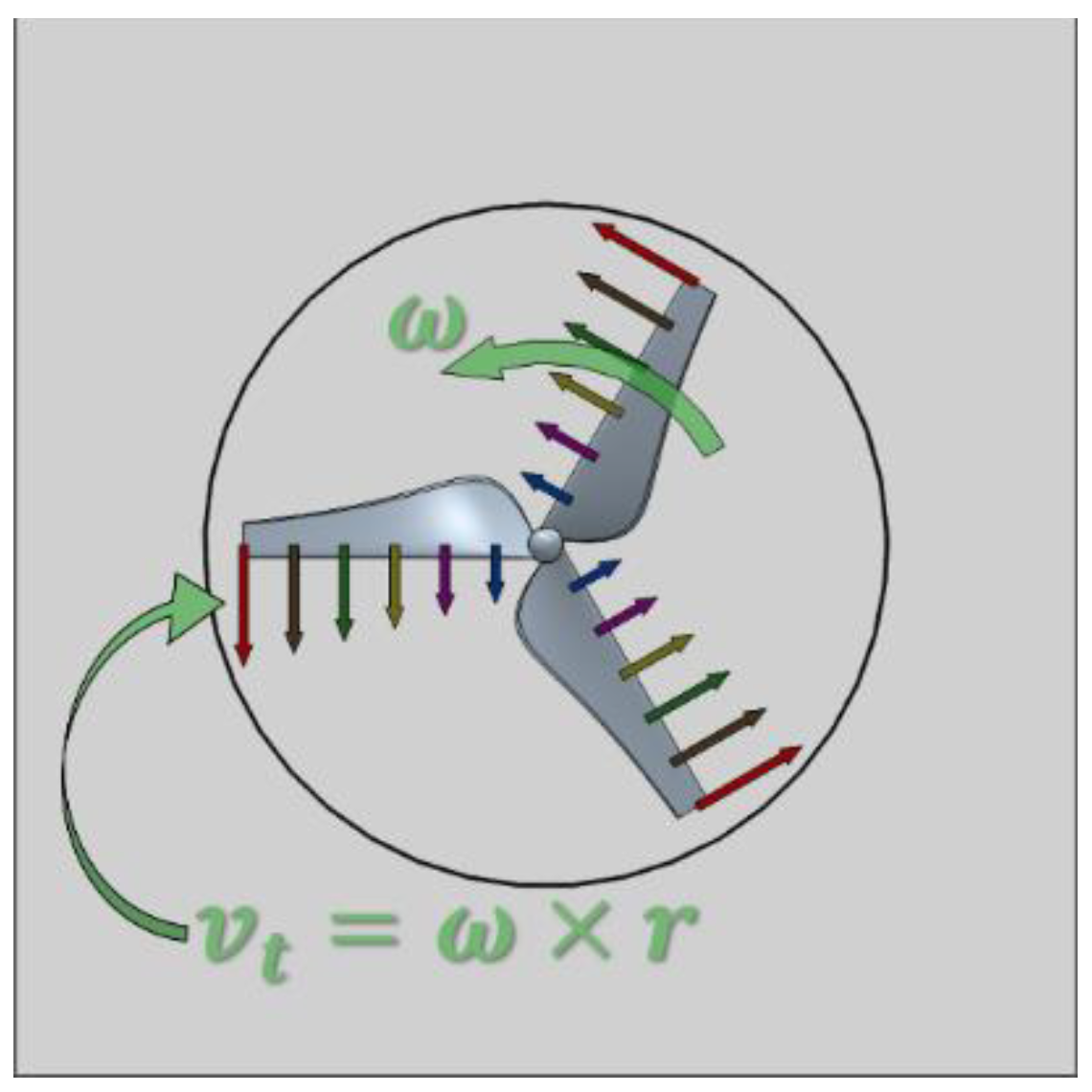
The frozen rotor approach is easily understandable if we simplify the whole mathematical approach for this technique into a rotating wall boundary condition. In this case, the solid body is rotating around its axis of rotation, while the velocity, near the wall, has an $\omega \times r$ component, where ω is the angular velocity and r is the distance from the axis of rotation. This method does not average the fluid quantities; thus, it provides nonuniform circumferential velocity, pressure, and turbulent quantities on the domain’s exiting face. In addition, the frozen rotor approach can be used during steady and unsteady simulations to simulate wake and vortex shedding.

The advantages of the frozen rotor interface are the following. The wake and the vortex shedding can be examined near the edges and near the blade tips. The disadvantage is that the relative position of the moving component is fixed; consequently, motion is modeled by adding the Coriolis and centrifugal forces to the momentum equation [21,22,23,24]. It is important to note that if performance such as quantities, such as torque, power, etc., are to be obtained, then the simulation must be repeated in different angular positions to eliminate the value dependency of each position [20,22].

The sliding mesh approach is a rotating motion interface, where there are also two domains: a stationary and a rotational one, similar to the previous methods. However, in this case, the rotational domain actually rotates. This approach can only be used in transient simulations due to the motion of the mesh. Among the three methods, the sliding mesh approach provides the most realistic results, but it requires the most computational resources too. Force, torque, and other quantities of the performance can be monitored during the time steps, and their values can be plotted against time or angular position.

Simplified explanatory diagrams about these modeling approaches are shown in the next figures (Figure 2, Figure 3 and Figure 4).

Commercial CFD software was used for the simulations (Simcenter STAR-CCM+ version V2022.1 from Siemens Digital Industries Software). A rectangle computational domain was employed with dimensions of 10D × 15D × 20D, where D denotes the diameter of the turbine (D = 200 mm). This computational domain has been tested in [28], and this size proved to be appropriate since neither was the computational cost high nor had the surrounding walls a significant effect on the numerical solution.

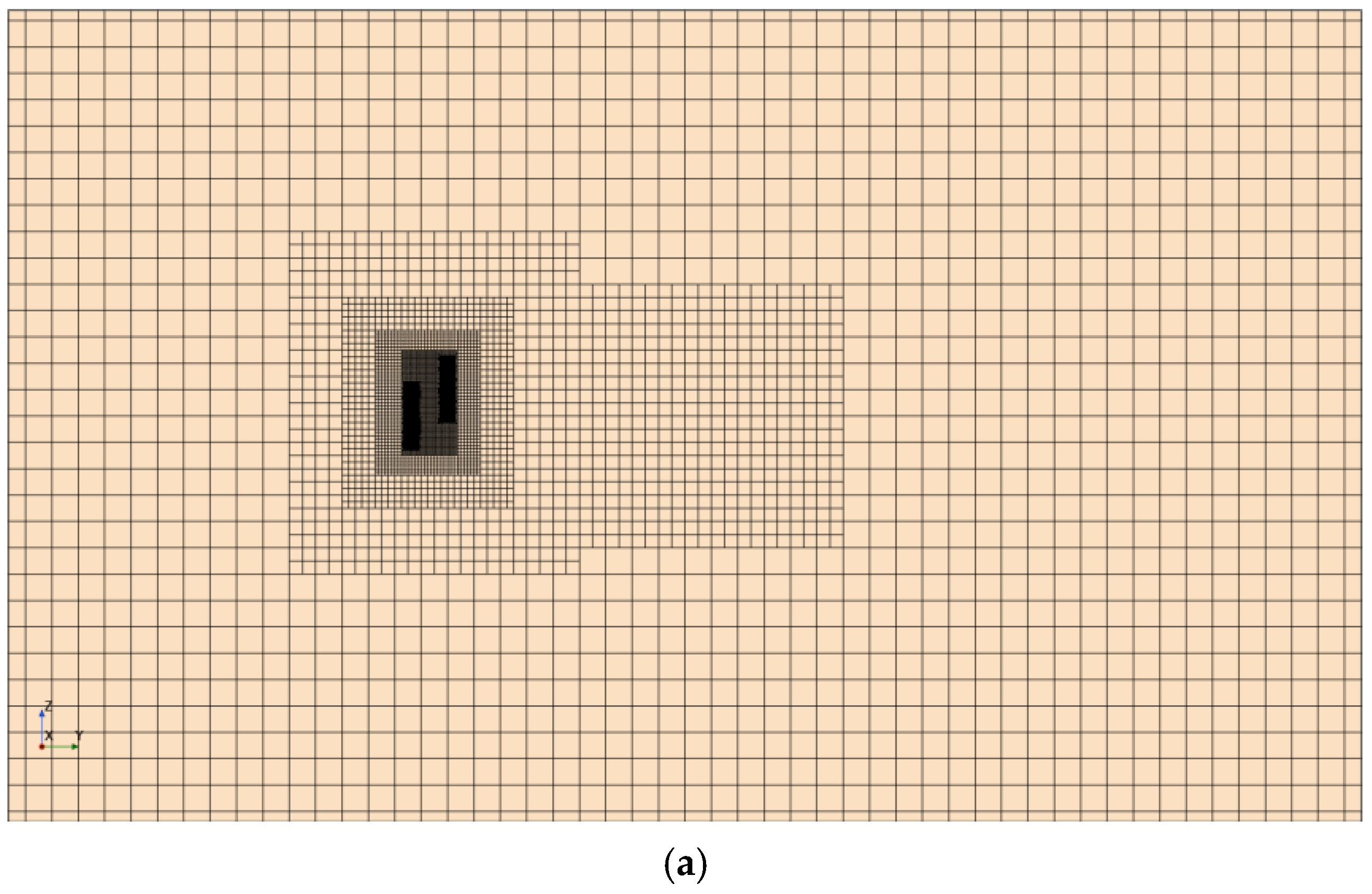
As for the rotors, the first one was positioned 7.5D from the “front” face and in the middle of the other two directions (10D from the sides). The domain with a cutout for the turbine is shown in the following Figure 5.

In the domain, the positions of the rotors were fixed. The distance between the rotors was 0.5D (100 mm) in both axial and radial directions. The turbines rotated in opposite directions, which is shown in the following Figure 6 with the rotors’ distances [29].

For the simulations, we used a segregated flow solver (SIMPLE), which solved the flow field and its quantities iteratively. The isotermic state and constant density were assumed for the fluid domain; therefore, only the continuity and the Navier–Stokes equations were solved. For modeling and simulating the turbulence, the SST k-ω turbulence model was used, which is described by the following equations:

$$\begin{array}{c}\frac{\partial \left(\rho ·k\right)}{\partial t}+div\left(\rho ·k·\mathit{U}\right)=div\left(\left(\mu +\frac{{\mu }_t}{{\sigma }_{\epsilon }}\right)·grad k \right)+P_k-{\beta }^{*}·\rho ·k·\omega \frac{\partial \left(\rho ·\omega \right)}{\partial t}\\ \frac{\partial \left(\rho ·\omega \right)}{\partial t}+div\left(\rho ·\omega ·\mathit{U}\right)=div\left(\left(\mu +\frac{{\mu }_t}{{\sigma }_{\omega ,1}}\right)·grad \omega \right)+{\gamma }_2\left(2·\rho ·S_{ij}·S_{ij}-\frac{2}{3}·\rho ·\omega ·\frac{\partial U_i}{\partial x_j}·{\delta }_{ij}\right)-\\ {\beta }_2·\rho ·{\omega }^2+2·\frac{\rho }{{\sigma }_{\omega ,2}·\omega }·\frac{\partial k}{\partial x_k}·\frac{\partial \omega }{\partial x_k}\end{array}$$

(6)

The inlet flow had a velocity of 3.79 m/s. On the sides of the domain, a symmetry boundary condition was applied, while a pressure outlet was employed on the outlet face. The ambient pressure was 1 atm (101,325 Pa). The fluid was “Air” from the material database of the Simcenter STAR-CCM+. The angular velocity of the domains was −1447.675 RPM and +1447.75 RPM; therefore, the tip speed ratio was 4 for each turbine.

To model the rotational motion, the previously presented approaches (frozen rotor, mixed plane, and sliding mesh) were used.

For the mixed plane approach in which the averaging was carried out within the rotating domain, only one geometry position was available since the rotated geometries provided the same results due to the averaging.

For the sliding mesh approach in which the simulation was transient, one geometry was used as well since, in this case, the mesh was rotating.

For the frozen rotor approach, seven different geometries were created, which were shifted by 15° between each step. The initial position (later referred to as position with 0°) is shown in Figure 7 and represented as white turbines. The rotated positions are represented with yellow and green colors, as the turbines were rotated by 15°. We used these 15° steps and directions for creating the seven different geometries in which the rotation angles were 0°, 15°, 30°, 45°, 60°, 75°, 90°, and 115°. The eighth position for 120° could be identical to 0° [30,31,32].

Before conducting the simulations, two kinds of dependency studies were carried out. The first one focused on determining the appropriate domain size, while the second one was for detecting mesh dependency. For the first series of simulations, various domain sizes were used and compared. In the mesh dependency study, six different meshes were employed, in which we compared the torque in each turbine. All simulations were steady state and utilized the boundary conditions described earlier with the initial (0°) geometry. The torque difference between the last two meshes was 3.8% and 1%. The change in the torque for the meshes is shown in Figure 8.

After the mesh dependency study, the last, viz. sixth mesh, was chosen for running our simulation. During the simulations, various quantities were monitored such as torque, pressure on the surface of the turbines, average and maximum velocities, and the residuals. While torque converged quickly, other quantities required more iterations to converge.

Despite using a mesh-independent grid, unexpected changes were observed in the torque; therefore, the simulations were carried out further on with adaptive mesh refinements (AMR) until 2500 iterations. A typical run is shown in Figure 9 below.

We can see in Figure 9 that the torque in each turbine started with an initial value, which converged rather fast to its final value at around 250–300th iterations. Following this, the torque remained constant until the 1400th iteration, at which point the first AMR was applied. The mesh refinement occurred after 100 iterations. Once the torque reached convergence, the simulation was stopped at the 2500th iteration.

The mesh that was used included two different meshing methods. In the “outer” region where the freestream is more dominant, a trimmed cell mesher was employed. Near the turbines and in the region of the turbines, a polyhedral mesher was used. The initial mesh is shown in Figure 10.

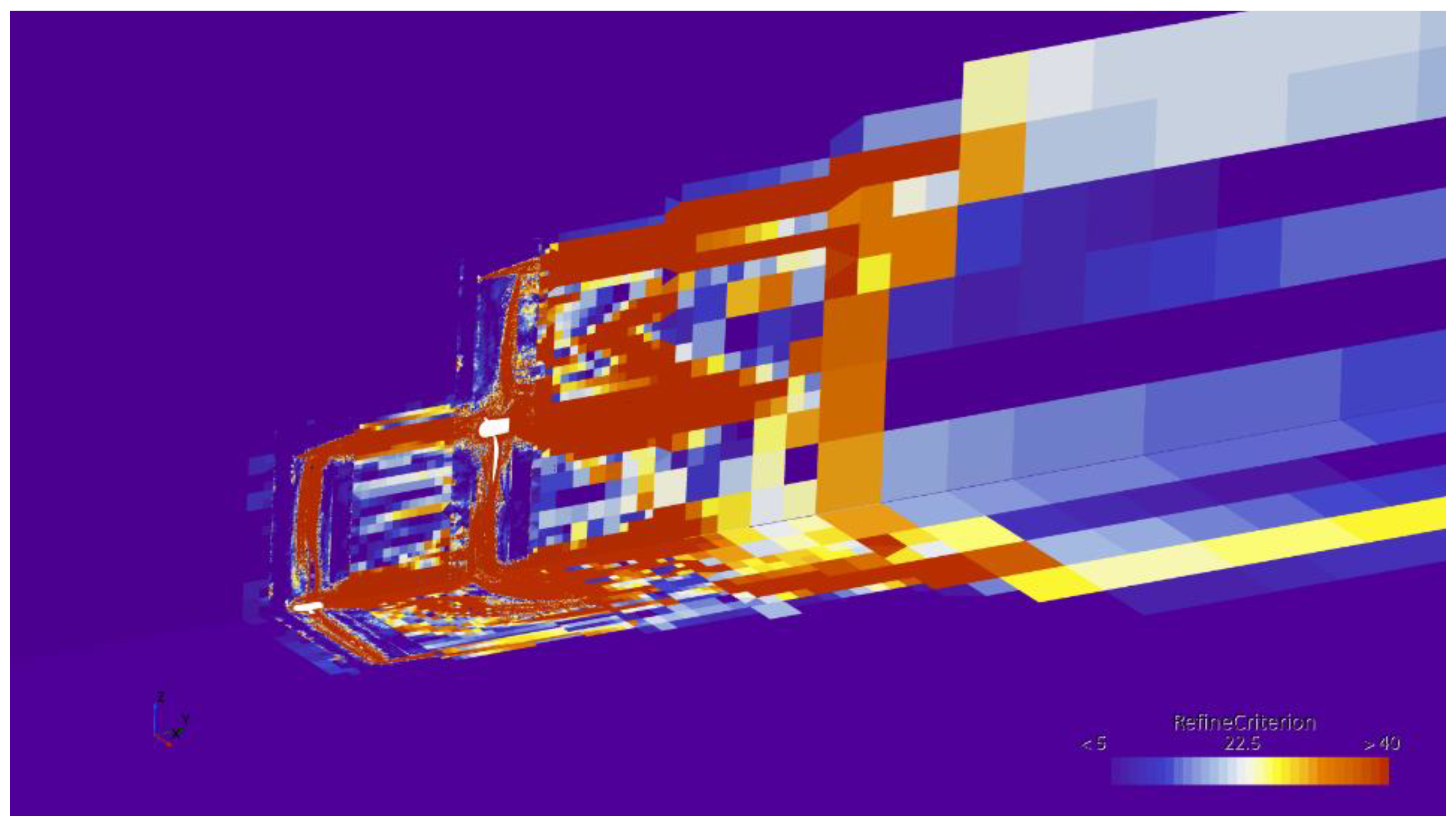
As previously mentioned, after the 1400th iteration, AMR was used. The last refined mesh (which was used for the 2500th iteration) for the 0° position is shown in Figure 11.

The grid contained prism mesh on the turbines with a mesh size of 0.02 mm. The prism layer mesh contained 15 layers, and the total thickness was 1 mm. The minimum adaptation cell size for the AMR was set to 0.45 mm. If this value was below 5, the AMR coarsened the mesh; if it was between 5 and 40, the mesh was not changed; and if its value was above 40, the AMR refined the mesh. The refinement criterion for the last iteration of the 0° position is shown in Figure 12.

For the position 0° at the 2500th iteration, the Y+ value and its distribution are shown in Figure 13. The average Y+ value on the first turbine was 0.4236, while the maximum and the minimum were 4.4453 and 0.0212, respectively. On the second turbine, the average of the Y+ was 0.4116, and the maximum and the minimum were 4.3640 and 0.0187, respectively. For the other positions, the values of the Y+ were similar.

During the mesh refinements of the AMR, the number of elements increased from approximately 6 million to 34 million, while the cell size decreased with each refinement. Although the element number increased dramatically, the torque did not change significantly.

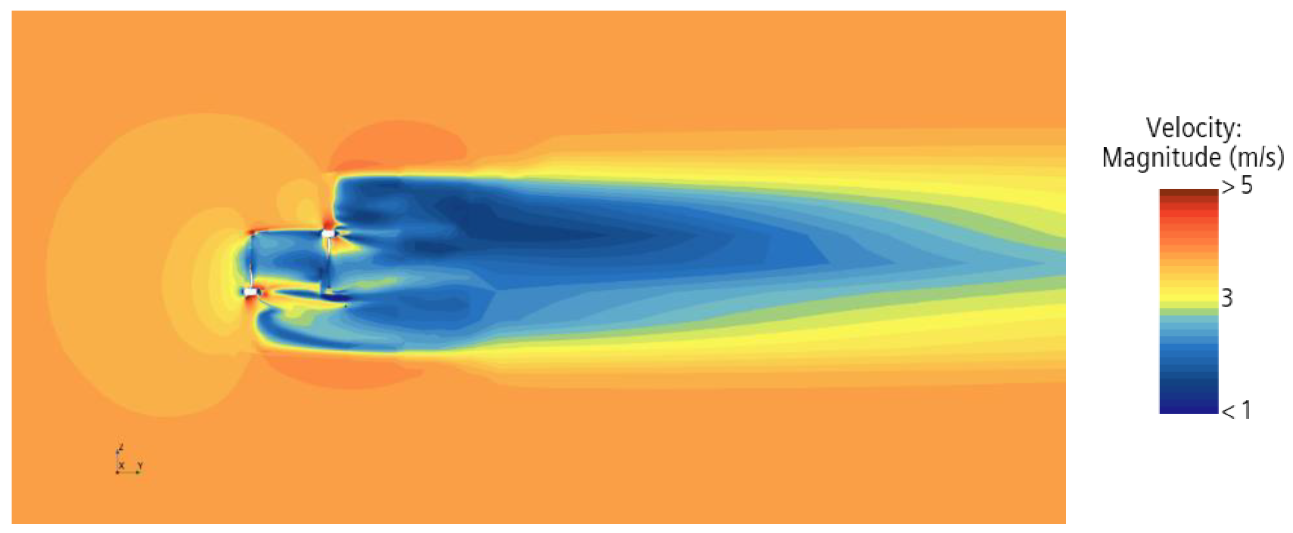
The velocity distribution near the turbine, for different positions, showed similar flow fields. Two wake regions for the two turbines, one between the two rotors and one larger after the second turbine, where the velocities were lower than the freestream velocity, were observed. However, for unsteady and frozen rotor cases, higher velocities near the tips could be detected due to the modeling of the rotating motion. Figure 14 shows the velocity distribution near the rotors for position 0°.

4. Results

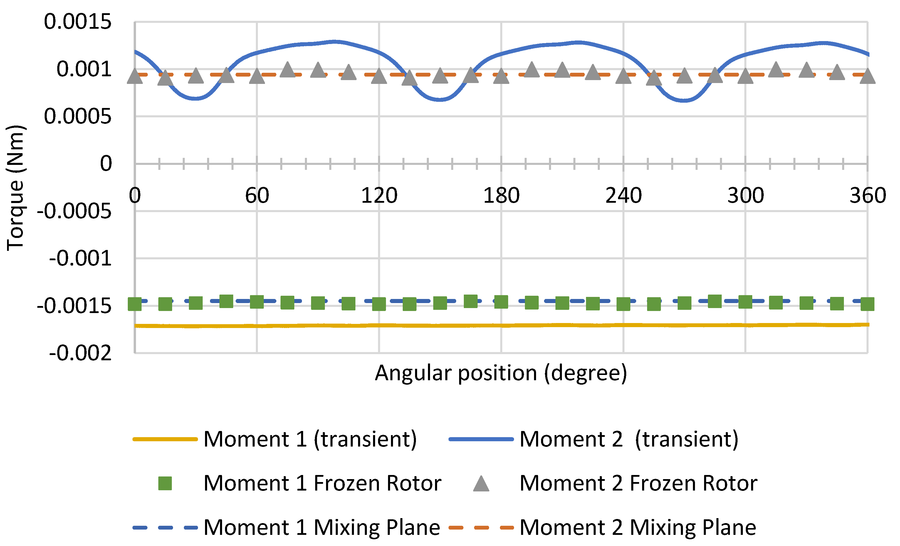
The three methods were compared in this article in the following way: calculation of torque on the turbine was carried out with the mixing plane and frozen rotor methods in a steady state, while the sliding mesh approach was in an unsteady state (Figure 15). The obtained data were compared to see how much the results obtained from the mixing plane and the frozen rotor approaches deviated if they were compared with the unsteady sliding mesh method.

In the case of the mixing plane method, the torque on the first turbine was −0.00145003 Nm, while on the second turbine, 0.000941719 Nm. The average torque with the frozen rotor technique was −0.001471612 Nm on the first turbine and 0.000946494 Nm on the second turbine. The average torque in the case of the sliding mesh method, between the fifth and the sixth revolutions, was −0.001707654 Nm and 0.001102037 Nm on the first and the second turbine, respectively.

When the torque obtained from the mixing plane and frozen rotor methods was compared to the averaged torque obtained from the sliding mesh method, then it can be seen that the steady-state solutions are 14–15% lower (

Table 1. Average torque on the rotors and their differences compared with the average of the transient result.

Method	Torque (Nm)	Percentage Difference Between Steady and Unsteady Torque (-)
Sliding mesh first rotor	−0.001707654	-
Sliding mesh second rotor	0.001102037	-
Mixing plane first rotor	−0.001450030	15.09%
Mixing plane second rotor	0.000941719	14.55%
Frozen rotor first rotor	−0.001471612	13.82%
Frozen rotor second rotor	0.000946494	14.11%

).

Based on the results, several conclusions have been made. First of all, it was expected that a higher difference would appear between the frozen rotor and the mixing plane methods since the second rotor behaved as a stator. Therefore, the impact of a stagnant rotor in the modeling was smaller than expected.

Second of all, it was also hypothesized that the frozen rotor method would yield similar results to the sliding mesh method, with the second turbine showing a sinusoidal (or other periodic) change; however, this phenomenon did not appear in the solution of the frozen rotor. It must also be mentioned that the difference between the torque with the mixing plane method and the average torque with the frozen rotor method was 1.47% and 0.50% on the first and second turbines, respectively. Consequently, the two methods provide closely identical solutions if similar engineering objects and phenomena (no tower and no ground) are modeled. Therefore, it is advisable to use the computationally cheaper method for these types of simulations.

Thirdly, the difference between the transient and steady-state results was higher than the difference between the steady-state results alone, with a difference of approx. 14–15% (using the average values as previously mentioned). The reason for this difference could be attributed to the different time domains (RANS vs. URANS) and the different rotating motion techniques (sliding mesh in a URANS simulation and steady rotating motion methods in a RANS simulation).

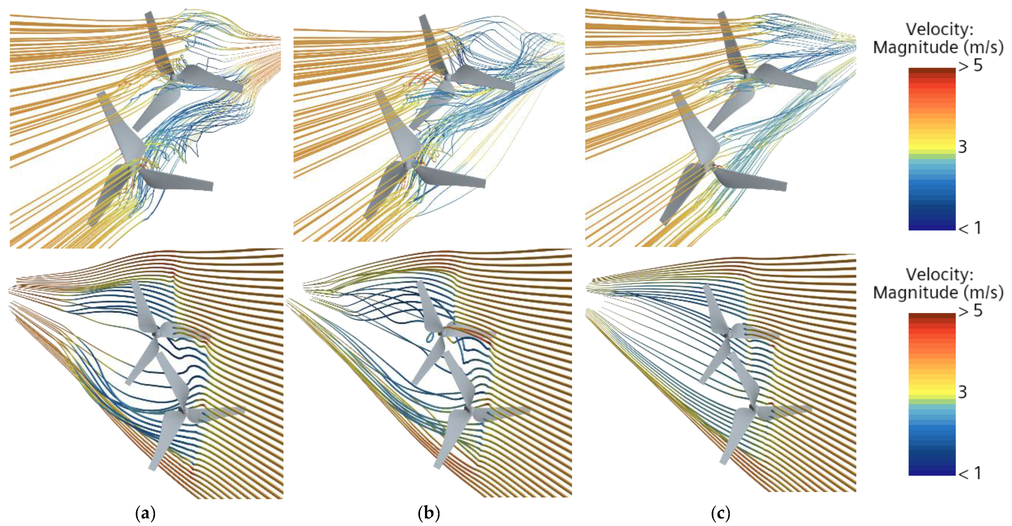
In addition to the conclusions, several important features, such as the streamlines or the turbulence-related vorticity, were also investigated.

With regard to the streamline (Figure 16), it is visible that the transient simulation (sliding mesh) and the frozen rotor solutions (steady state) have similar results near the turbine; however, the time-dependent solution has more vortexes than the steady solution. The other steady solution with the mixing plane approach has a “smoother” result, which means that the streamlines have a swirl after turbines due to the averaging.

With regard to vorticity (Figure 17), the so-called Q criterion at Q = 800 1/s² value was used to model the differences between the methods.

Figure 17a shows a fluid structure starting from the first turbine’s tip and colliding with the second turbine in the sliding mesh simulation. In this case, it is possible to find another turbulence structure, which starts from the second turbine and flows “back”.

The second picture in Figure 17b shows a less consistent swirling structure starting from the tip of the blades, which can also be found in the sliding mesh simulation. Due to RANS/URANS differences, a vortex appears that starts from the tip of the blade and flows straight “back”, which is also visible in Figure 17b.

The third picture in Figure 17c shows the mixing plane approach, which shows neither a turbulence structure such as the result obtained from the sliding mesh nor the ones obtained from the frozen rotor approach. This indicates that the mixing plane approach averages out the turbulences, as mentioned in the introduction.

In the case of numerical methods, it is advisable to mention the computational costs as well.

Two steady-state simulations (mixing plane and frozen rotor) were compared to a transient simulation (sliding mesh). Three simulations were carried out with the same mesh settings for comparing the computational resources. Although the same mesh settings were used for the three methods, different cell numbers were generated due to their distinct characteristics.

For the mixing plane method, 4,622,698 cell numbers were generated, while for the frozen rotor, 6,109,872, and for the sliding mesh approach, 6,112,514. The difference between the frozen rotor and the sliding mesh comes from the meshers and their tolerances, while the difference between the mixing plane and the other two approaches comes from the differences in the rotating domain’s interfaces.

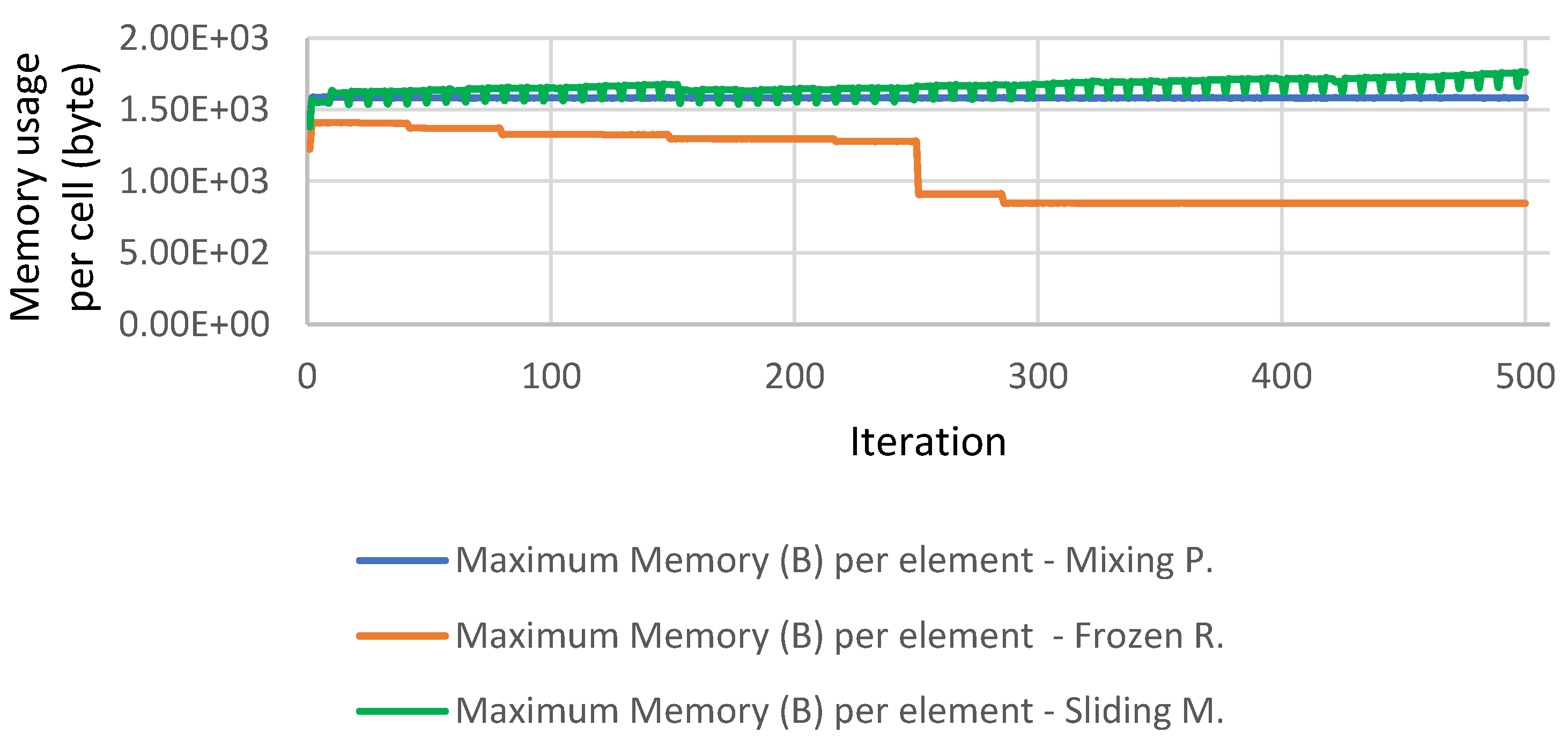
Computational costs were examined based on memory usage per cell and time requirement per cell.

With regard to memory usage per cell, it can be generally observed that the sliding mesh solution has some periodicity due to its solving method, which appears in every eighth iteration (Figure 18). The explanation for this periodicity is that the SIMPLE algorithm was used, which has a fixed number (8) of inner iterations. After this inner iteration number, the solver jumped to the next time step and calculated eight iterations within that time step to decrease the residual error. It must be mentioned that a growing trend in memory usage can be noticed as time changes.

In the case of the frozen rotor method, the memory usage was constant, while the memory usage decreased in the case of the mixing plane until it reached 300 iterations, then it became constant. In numbers, the average memory usage for the mixing plane simulation was 1588.247791 bytes/element, for the frozen rotor approach, 1409.438993 bytes/element, while for the sliding mesh solution, 1761.482633 bytes/element.

With regard to the time requirement per cell, steady solutions had similar time requirements for one iteration. Since the meshing numbers were different, the time requirement was calculated for one iteration per element, which is shown in Figure 19.

During the first 500 iterations, the average time requirement for one iteration per cell was 3.11816 × 10⁻⁵ s for the mixing plane solution, 1.40947 × 10⁻⁵ s for the frozen rotor, and 1.18686 × 10⁻⁹ s for the sliding mesh method.

5. Validation

The validation was carried out by comparing the experimentally [28] and numerically obtained pressure coefficient (c_p) as a function of the tip speed ratio. The experiment was performed with 3D-printed turbine blades in a wind tunnel equipped with a HELIOS HQ630-type fan. For the initial position, the two turbines were positioned in a way that the blades would turn toward each other; therefore, the first turbine did not block the wind from the second turbine. We applied the frozen rotor method in the simulation (Figure 20).

As it is visible, the numerically obtained results are in accordance with the experimental ones. Therefore, it can be concluded that the numerical model, with its boundary conditions, is well established and feasible to use.

6. Summary

In this paper, modeling methods were examined to recognize which approach fits the most for counter-rotating dual-rotor wind turbine (CO-DRWT) applications.

In this regard, simulation settings, including the domain shape and size, physical models, boundary conditions, and mesh, were discussed in detail. This was followed by a comparison of the obtained results from the mixing plane, frozen rotor, and sliding mesh approaches. Although it was initially hypothesized that the frozen rotor method would provide significantly different torque compared with the sliding mesh approach, the actual results were highly similar compared with both the mixing plane and the sliding mesh methods. In addition, it was concluded that the rotor–stator effect for a CO-DRWT is negligible or nonexistent with our half-diameter axial and half-diameter radial shifts. The torque obtained with the mixing plane and frozen rotor approaches were highly similar.