GTMesh: A Highly Efficient C++ Template Library for Numerical Schemes on General Topology Meshes

Abstract

This article introduces GTMesh, an open-source C++ library providing data structures and algorithms that facilitate the development of numerical schemes on general polytopal meshes. After discussing the features and limitations of the existing open-source alternatives, we focus on the theoretical description of geometry and the topology of conforming polytopal meshes in an arbitrary-dimensional space, using elements from graph theory. The data structure for mesh representation is explained. The main part of the article focuses on the implementation of data structures and algorithms (computation of measures, centers, normals, cell coloring) by using State-of-the-Art template metaprogramming techniques for maximum performance. The geometrical algorithms are designed to be valid regardless of the dimension of the underlying space. As an integral part of the library, a template implementation of class reflection in C++ has been created, which is sufficiently versatile and suitable for the development of numerical and data I/O algorithms working with generic data types. Finally, the use of GTMesh is demonstrated on a simple example of solving the heat equation by the finite volume method.

1. Introduction

Numerical algorithms for the solution of problems for partial differential equations often rely on meshes covering the computational domain. The prominent representatives of mesh-based methods are the finite element method (FEM) [1,2,3,4] and the finite volume method (FVM) [5,6,7]. In order to tackle domains with nontrivial geometries, efficient tools for unstructured mesh representation and manipulation are needed. In particular, using general polygonal or polyhedral meshes comprising a relatively small number of highly complex cells can be beneficial in several situations.

Using FVM to solve problems involving, e.g., reacting multiphase flows [8,9], the number of necessary evaluations of computationally costly terms in the governing equations can be reduced by using polyhedral meshes. In the CFD domain, the properties of polyhedral meshes and their possible advantages, in terms of convergence rate and computational costs, have recently started to be investigated systematically [10,11,12,13], and their support is available in popular packages, such as ANSYS Fluent, OpenFOAM [14] or AVL FIRE. Efficient finite volume schemes, specifically tailored to polyhedral meshes, are in active development [15,16].

FEM traditionally uses tetrahedral or hexahedral meshes (in 3D). However, FEM has recently been successfully generalized to meshes of convex polyhedrons, which has brought about significant advantages [17,18,19,20]. Their applications also extend to computer graphics [21].

For developers of numerical codes, several open-source projects offer mesh handling support, but none of them can provide the complete set of features required by high-performance parallel FVM and FEM codes. Notable examples are outlined below:

• OpenMesh [22] is aimed at applications in computer graphics, and provides tools for mesh modification. However, it only supports polygonal meshes for the representation of surfaces in 3D.
• PUMI (Parallel Unstructured Mesh Infrastructure) [23] is a complex library supporting distributed mesh storage and processing via MPI [24]. By default, the mesh representation by means of the MDS (Mesh Data Structure) submodule only accepts a limited set of topological types known a priori at compile time, in order to achieve high performance.
• ViennaGrid [25] is a modern library leveraging the concepts of template metaprogramming and iterators available in C++. It provides data structures for arbitrary-dimensional meshes and also a number of specialized data types and mesh algorithms that are often limited to certain dimensions or mesh types.
• MOAB (Mesh-Oriented datABase) [26] is an extensive library that allows general topology meshes and supports mesh refinement, decomposition, parallel I/O and other features. Despite being written in C++, it does not take advantage of templates, and its performance has been shown to be relatively poor when processing polyhedral meshes [27]. MOAB always represents mesh geometry in a 3D coordinate system.
• DUNE (Distributed and Unified Numerics Environment) [28] is a framework for numerical computations primarily (but not exclusively) aimed at FEM. It is a mature and very complex project with incomplete documentation, which also supports general topology meshes.
• TNL (Template Numerical Library) [29] is a dynamically evolving framework for implementing efficient numerical algorithms in C++, taking advantage of State-of-the-Art C++ programming paradigms and exposing both CPU and GPU programming through a unified interface. Recently, support for general topology polytopal meshes [27] has been added.

With all the above in mind, we introduce GTMesh, a library created to facilitate rapid development of numerical schemes and data postprocessing algorithms on general polytopal meshes in an arbitrary dimension. GTMesh is implemented as a modern C++ header-only library (compliant with the C++14 standard [30]). GTMesh makes extensive use of template metaprogramming, together with advanced concepts, such as SFINAE [31], on account of which it can provide generic data structures and mesh algorithms that compile for the desired use case and provide maximum run time performance. Using GTMesh, it is possible to write the dimension-agnostic code of a complete numerical solver, including the numerical scheme, the data association with the mesh and the data I/O. The dimension of the problem is then specified as a template parameter at a single point in the code. Currently, GTMesh is a relatively small open-source project, which is publicly available, together with introductory documentation (see Data Availability Statement at the end).

This paper serves as an introduction to the concepts used in GTMesh. In Section 2, the theoretical description of general topology meshes in ${\mathbb{R}}^d$, $d\in \mathbb{N}$, is laid out. Section 3 presents the general data structure for the mesh representation used in this project. The implementation details are explained in Section 4, including the data structures (Section 4.1 and Section 4.2) and the mesh algorithms (Section 4.3). In this section, the ideas are often presented in the context of FVM schemes. For simplicity, geometrical considerations are demonstrated on 2D polygons or 3D polyhedra, despite the possibility of generalization into ${\mathbb{R}}^d$, $d>3$. Section 5 is devoted to a useful concept of class reflection, which finds utility in generic numerical and data I/O algorithms. Its implementation is based on original ideas combining C++ class templates and preprocessor macros, in order to create a transparent and comfortable interface for the user. Finally, a simple example program that solves heat conduction in 3D, by the FVM scheme, is demonstrated in Section 6.

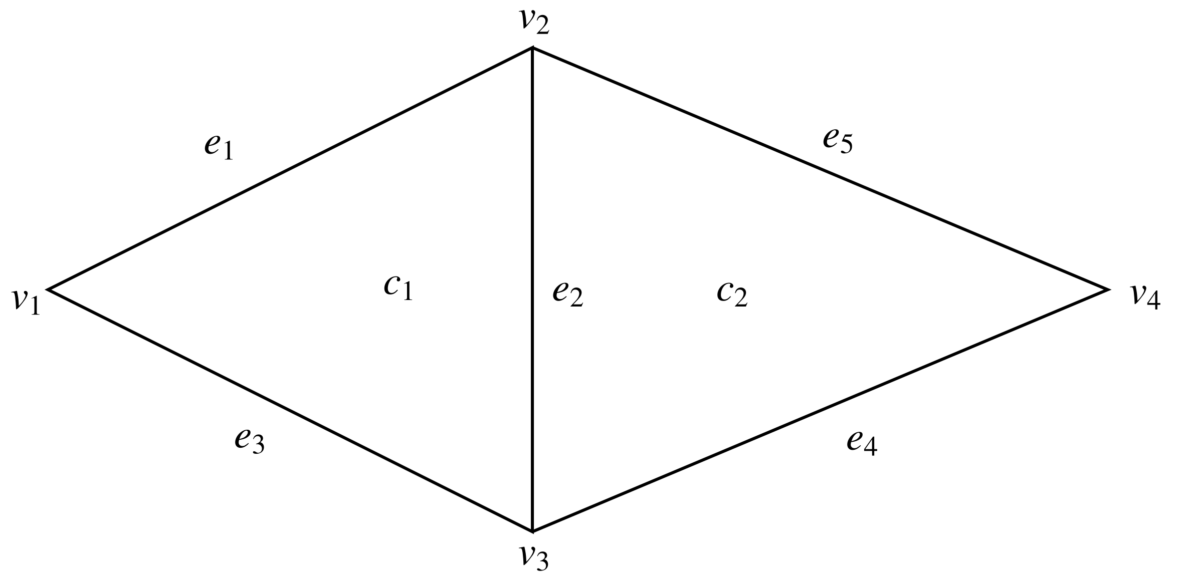
2. Geometry and Topology of Unstructured Meshes

The following definitions are motivated by meshing computational domains for the purpose of finite volume schemes. For an arbitrary set, $S\subset {\mathbb{R}}^d$, denoted by $m\left(S\right)$, the d-dimensional Lebesgue measure of S, and by $\tilde{m}\left(S\right)$, the $\left(d-1\right)$-dimensional Hausdorff measure of S.

Definition 1.

Let the spatial domain Ω be a bounded polytope in ${\mathbb{R}}^d$, $d\in \mathbb{N}$. Let $\mathcal{T}$ be a set of polytopal cells, and denote by $\mathcal{E}$ the set of all faces that constitute the boundaries of all elements of $\mathcal{T}$. $\mathcal{T}$ is called a d-dimensional conforming mesh on Ω, if the following properties are satisfied:

• $\overline{{\bigcup }_{K\in \mathcal{T}}K}=\overline{\Omega }$.
• $\left(\forall K\in \mathcal{T}\right)\left(\exists {\mathcal{E}}_K\subset \mathcal{E}\right)\left(\partial K={\bigcup }_{\sigma \in {\mathcal{E}}_K}\overline{\sigma }\right)$.
• $\left(\forall K,L\in \mathcal{T}\right)\left(K\ne L\Rightarrow \left(\tilde{m}\left(\overline{K}\cap \overline{L}\right)=0\vee \left(\exists \sigma \in \mathcal{E}\right)\left(\sigma =\overline{K}\cap \overline{L}\right)\right)\right)$.

Next, we introduce the notation for the sets of elements of different dimensions that form the geometry of the mesh. For example, in a 3D mesh, the boundaries of the 3D cells consist of 2D faces, which in turn represent flat surfaces bounded by 1D edges, which in turn span between their two 0D vertices. In order to avoid confusion with the notion of element in FEM, these objects are also called entities [27].

Definition 2.

Let $\mathcal{T}$ be a d-dimensional mesh, where $d\in \mathbb{N}$. The set of elements of dimension $k\in$$\left\{0,1,\dots ,d\right\}$ is denoted by ${\mathcal{T}}^k$. $N_{\mathcal{T}}^k=\left|{\mathcal{T}}^k\right|$ is the number of elements of dimension k in $\mathcal{T}$. Finally, the complete system of geometrical elements is defined as

$${\mathcal{T}}^{*}=\bigcup _{k=0}^d{\mathcal{T}}^k.$$

By Definition 2, we have $\mathcal{E}={\mathcal{T}}^{d-1}$. In terms of the mutual inclusion of elements of various dimensions, we define the relation of connection on ${\mathcal{T}}^{*}$:

Definition 3.

$e,f\in {\mathcal{T}}^{*}$ are connected ⟺$\left(e\subset \overline{f}\vee f\subset \overline{e}\right)$.

An example of mesh connections can be seen in Figure 1.

Figure 1. Example of connections in a simple 2D mesh. Vertices connected to element $c_1$ are $\left\{v_3,v_2,v_4\right\}$. The cells connected to element $v_1$ are $\left\{c_1,c_2\right\}$.

Figure 1. Example of connections in a simple 2D mesh. Vertices connected to element $c_1$ are $\left\{v_3,v_2,v_4\right\}$. The cells connected to element $v_1$ are $\left\{c_1,c_2\right\}$.

In a similar intuitive way, the neighborhood of elements is defined:

Definition 4.

Let $e\in {\mathcal{T}}^{*}$. Then, the neighborhood of e is defined as

$$N\left(e\right)=\left\{e^{\prime }\in {\mathcal{T}}^{*}\left|e^{\prime }\mathrm{is}\mathrm{connected}\mathrm{to}e\right.\right\}.$$

Moreover, we denote the subset of the connected elements with the given dimension $k\in \left\{0,1,\dots ,d\right\}$ as

$$N^k\left(e\right)=N\left(e\right)\cap {\mathcal{T}}^k.$$

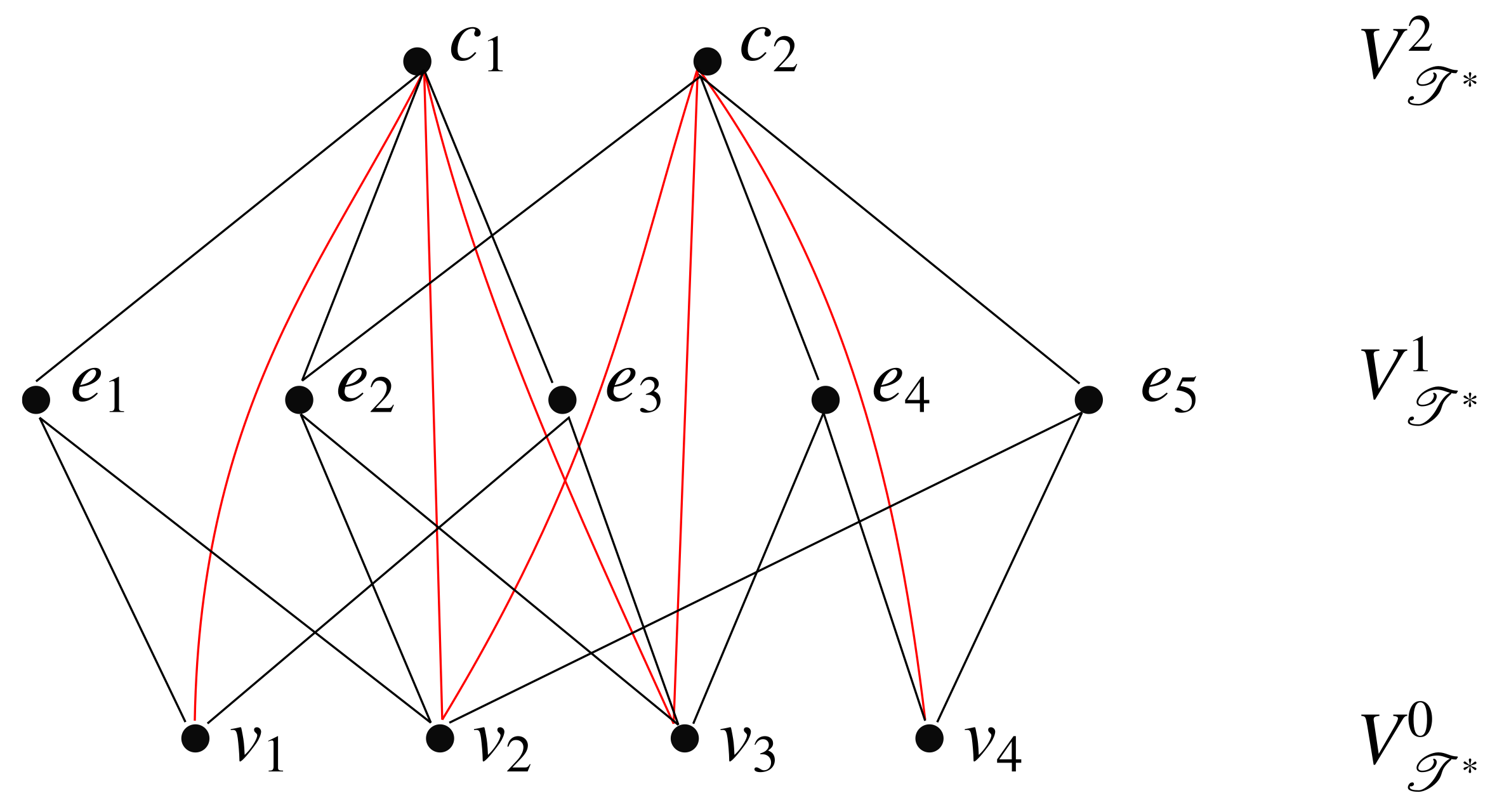
Graph Description of a General Topology Mesh

All connections in the mesh can be represented by means of a graph $G_{{\mathcal{T}}^{*}}=(V_{{\mathcal{T}}^{*}},E_{{\mathcal{T}}^{*}})$, where the vertices of the graph match the elements of the mesh, and where the edges of the graph correspond to the connections between them. The vertices $V_{{\mathcal{T}}^{*}}$ of $G_{{\mathcal{T}}^{*}}$ are grouped into layers by dimensions of elements:

$$\begin{array}{cc}\hfill V_{{\mathcal{T}}^{*}}& \cong {\mathcal{T}}^{*}={\mathcal{T}}^0\cup {\mathcal{T}}^1\cup \dots \cup {\mathcal{T}}^d;\hfill \end{array}$$

(1)

$$\begin{array}{cc}\hfill V_{{\mathcal{T}}^{*}}^k& \cong {\mathcal{T}}^k.\hfill \end{array}$$

(2)

The edges of $G_{{\mathcal{T}}^{*}}$ are defined as

$$E_{{\mathcal{T}}^{*}}=\left\{\left(e,e^{\prime }\right)\in V_{{\mathcal{T}}^{*}}^2\left|e,e^{\prime }\mathrm{are}\mathrm{connected}\right.\right\}.$$

(3)

For an example, see Figure 2.

The graph $G_{{\mathcal{T}}^{*}}$ contains all information about the topology of the mesh. As the connection of elements is a symmetrical relation, the graph $G_{{\mathcal{T}}^{*}}$ is de facto undirected, i.e., $\left(e,e^{\prime }\right)\in E_{{\mathcal{T}}^{*}}⟺\left(e^{\prime },e\right)\in E_{{\mathcal{T}}^{*}}$, $\forall e,e^{\prime }\in V_{{\mathcal{T}}^{*}}$. Additionally, for a simpler description of the connections, i.e., of the graph edges, we denote a subset of graph edges from dimension $d_1$ to dimension $d_2$ as

$$E_{{\mathcal{T}}^{*}}^{d_1,d_2}=\left\{\left(e,e^{\prime }\right)\in E_{{\mathcal{T}}^{*}}\left|e\in V_{{\mathcal{T}}^{*}}^{d_1},e^{\prime }\in V_{{\mathcal{T}}^{*}}^{d_2}\right.\right\}.$$

(4)

Definition 5.

Let $G=\left(V,E\right)$ be a graph. The adjacency matrix of the graph G is matrix ${\mathbb{A}}_G\in {\mathbb{R}}^{\left|V\right|\times \left|V\right|}$, defined as

$${\left[{\mathbb{A}}_G\right]}_{ij}=\left\{\begin{array}{c}1\mathit{if}\left(v_i,v_j\right)\in E,\\ 0\mathit{if}\left(v_i,v_j\right)\notin E,\end{array}\right.$$

(5)

where $i, j\le \left|V\right|$, $v_i, v_j\in V$.

Furthermore, to investigate certain types of connections and properties of the graph mesh representation, we introduce the idea of a connection matrix, closely related to the adjacency matrix. The connection matrix from dimension $d_1$ to dimension $d_2$ reads

$${\left[{\mathbb{A}}_{G_{{\mathcal{T}}^{*}}}^{d_1,d_2}\right]}_{ij}=\left\{\begin{array}{c}1\mathrm{if}\left(v_i,v_j\right)\in E,v_i\in V_{{\mathcal{T}}^{*}}^{d_1},v_j\in V_{{\mathcal{T}}^{*}}^{d_2},\\ 0\mathrm{if}\left(v_i,v_j\right)\notin E,v_i\in V_{{\mathcal{T}}^{*}}^{d_1},v_j\in V_{{\mathcal{T}}^{*}}^{d_2},\end{array}\right.,$$

(6)

where ${\mathbb{A}}_{G_{{\mathcal{T}}^{*}}}^{d_1,d_2}\in {\mathbb{R}}^{N_{\mathcal{T}}^{d_1}\times N_{\mathcal{T}}^{d_2}}$. The connection matrix is a rectangular block of $A_{G_{{\mathcal{T}}^{*}}}$.

The primary aim of the data structure representing any unstructured mesh is to store all connections of the elements in the mesh. Equivalently, it must contain enough information for the reconstruction of the whole $G_{{\mathcal{T}}^{*}}$. The graph is fully described by its adjacency matrix. Due to certain properties of the adjacency matrix of $G_{{\mathcal{T}}^{*}}$, it is possible to reduce the amount of connections stored. First, it holds that

$${\left({\mathbb{A}}_{G_{{\mathcal{T}}^{*}}}^{d_1,d_2}\right)}^T=\left({\mathbb{A}}_{G_{{\mathcal{T}}^{*}}}^{d_2,d_1}\right),$$

(7)

where the ${\mathbb{A}}_{G_{{\mathcal{T}}^{*}}}^{d_1,d_2}\in {\left\{0,1\right\}}^{\left|V_{{\mathcal{T}}^{*}}^{d_1}\right|\times \left|V_{{\mathcal{T}}^{*}}^{d_2}\right|}$ is a rectangular submatrix of ${\mathbb{A}}_{G_{{\mathcal{T}}^{*}}}$ reflecting the connections from ${\mathcal{T}}^{d_1}$ to ${\mathcal{T}}^{d_2}$. The second property is the dependence between adjacency matrices between specified dimensions. The relation reads

$$\begin{array}{cc}\hfill {\left[{\mathbb{A}}_{G_{{\mathcal{T}}^{*}}}^{d_1,d_2}\right]}_{ij}& =\mathrm{connect}\left({\mathbb{A}}_{G_{{\mathcal{T}}^{*}}}^{d_1,d_3},{\mathbb{A}}_{G_{{\mathcal{T}}^{*}}}^{d_3,d_2}\right)\hfill \\ \hfill & =\left\{\begin{array}{cc}1& \mathrm{if}\left(\exists k\in \left\{1,2,\dots ,N_{{\mathcal{T}}^{*}}^{d_3}\right\}\right)\left({\left[{\mathbb{A}}_{G_{{\mathcal{T}}^{*}}}^{d_1,d_3}\right]}_{ik}{\left[{\mathbb{A}}_{G_{{\mathcal{T}}^{*}}}^{d_3,d_2}\right]}_{kj}=1\right),\\ 0& \mathrm{else},\end{array}\right.\hfill \end{array}$$

(8)

where the dimensions $d_1,d_2,d_3$ satisfy $\left(d_1>d_3>d_2\right)\vee \left(d_1<d_3<d_2\right)$. In other words, the Formula (8) represents the chaining of the connections in the graph. The condition for the dimensions of the connection matrices consists in finding the correct paths in the graph that are consistent with the mesh topology.

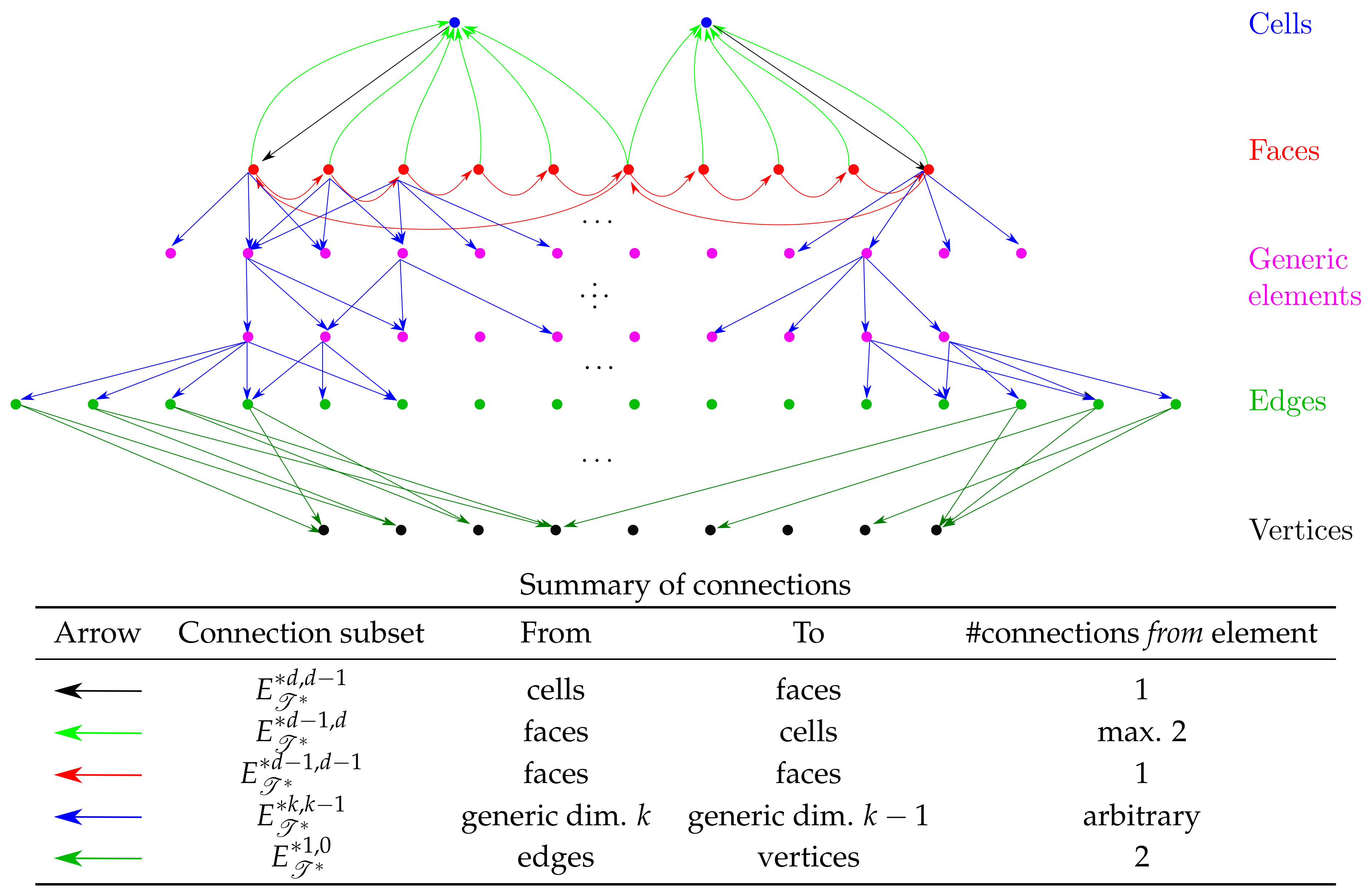
3. Abstract Data Structure for Mesh Representation in ${\mathbb{R}}^{\mathit{d}}$

This section describes the system of connections used in this work for storing an unstructured mesh with general topology and dimensions.

According to (7) and (8), it is necessary to store either connections from $V_{{\mathcal{T}}^{*}}^k$ to $V_{{\mathcal{T}}^{*}}^{k-1}$ or from $V_{{\mathcal{T}}^{*}}^{k-1}$ to $V_{{\mathcal{T}}^{*}}^k$, because those connections cannot be correctly obtained otherwise. Therefore, we introduce a basic data structure as a sub-system of connections suitable to represent any unstructured mesh in any dimension. Let us first consider the case $d=3$. The chosen data structure in 3D stores the connections

$$E_{{\mathcal{T}}^{*}}^{*}=E_{{\mathcal{T}}^{*}}^{*3,2}\cup E_{{\mathcal{T}}^{*}}^{*2,2}\cup E_{{\mathcal{T}}^{*}}^{2,3}\cup E_{{\mathcal{T}}^{*}}^{2,1}\cup E_{{\mathcal{T}}^{*}}^{1,0},$$

(9)

where the $E_{{\mathcal{T}}^{*}}^{*3,2}$ and $E_{{\mathcal{T}}^{*}}^{*2,2}$ are auxiliary connections enabling direct iteration over cell boundaries. The $E_{{\mathcal{T}}^{*}}^{*3,2}$ are pointers from each cell to one of its faces, while the references $E_{{\mathcal{T}}^{*}}^{*2,2}$ are between the faces, and they connect the faces making up the boundary of each single cell. Other connections are defined according to Equation (4). For better understanding of the connections between the elements, see Figure 3 presenting connections in a 3D mesh.

This concept is extensible to any dimension. The formula describing the system of connections stored in d-dimensional unstructured mesh is

$$E_{{\mathcal{T}}^{*}}^{*}=E_{{\mathcal{T}}^{*}}^{*d,d-1}\cup E_{{\mathcal{T}}^{*}}^{*d-1,d-1}\cup E_{{\mathcal{T}}^{*}}^{d-1,d}\cup E_{{\mathcal{T}}^{*}}^{d-1,d-2}\cup \dots \cup E_{{\mathcal{T}}^{*}}^{2,1}\cup E_{{\mathcal{T}}^{*}}^{1,0}.$$

(10)

The system of connections $E_{{\mathcal{T}}^{*}}^{*}$ is presented in Figure 4.

4. The GTMesh Library

The GTMesh library is a C++ project designed for efficient work with polytopal meshes. In order to achieve both user friendliness and computational efficiency, it utilizes modern C++ paradigms. The architecture of GTMesh aims at maintainability and extensibility, using, e.g., the open–closed principle [32].

From the construction point of view, the internal structure of the mesh storing the chosen system of connections (10) is very similar to formats of sparse matrices. However, the structures representing elements are designed to be more convenient for the user.

The library provides commonly used mesh algorithms determining, e.g., connections between elements of any desired dimensions, neighborhood of elements, measures of all elements of a mesh of an arbitrary dimension and normals to cell faces.

The architecture of GTMesh is split into four main parts:

• storing the mesh topology;
• associating data with the mesh;
• calculating various properties of the mesh;
• exporting and importing mesh-related data.

The construction parts of GTMesh are described in the following sections. Section 4.1 discusses the structure storing the mesh topology. Section 4.2 presents the system of data mapping to the mesh. This data mapping system significantly contributes to the user friendliness of GTMesh. Next, the auxiliary functions for calculating, e.g., elements centers and measures are described in Section 4.3. Section 5 describes a unique system of class reflection, developed to automate basic operations with C++ structures or classes such as serialization, deserialization or arithmetical operations. This concept improves the development efficiency, as it reduces the amount of routine work on data interface coding.

4.1. Mesh Data Structure

The complete C++ data structure storing a mesh consists of arrays containing the mesh elements. The representation of a mesh element is to be understood as a simple C++ data structure containing the respective references from (10). An example for the dimension $d=3$ is depicted in Figure 5. In addition, the structures for cells and faces contain two auxiliary data elements: center (see Section 4.3) and flag.

The elements are collected in a data structure called MeshElements, which is de facto the unstructured mesh itself. Due to the template implementation of the mesh element data structure, it is possible to automatically generate the system of elements based on the template arguments, i.e., only one definition of the MeshElements class is required, e.g., for definitions of 2D or 3D mesh. The dimension of the mesh is given by a template parameter.

Additionally, it is possible to prescribe the maximum number of sub-elements of faces and other elements which have references represented by blue arrows in Figure 4. This number is called Reserve. When Reserve is defined, it is possible to embed the references directly into the corresponding mesh element data structure, avoiding dynamic memory allocation. For example, when the number of sub-elements of faces in a 3D mesh is prescribed to three, the stored mesh can only have triangular faces. Note that, due to the chosen representation, the number of faces of one cell is unlimited in any dimension.

4.2. Associating Data with the Mesh

Any numerical method for solving a system of partial differential equations on a domain tessellated by the mesh needs to store data associated with the individual mesh elements. The data can represent the values of the solution, auxiliary pre-calculated space-dependent quantities or implementation-specific storage for intermediate results. The purpose (and hence the type) of data associated with mesh elements is specific to their dimension. For example, finite volume methods use solution values for the computationally significant elements, i.e., cell centers, cell faces or both. However, additional data storage may be allocated, for each vertex to hold the results of intermediate calculations.

GTMesh provides a data container, named MeshDataContainer, to conveniently store data associated with mesh elements. Once the mesh geometry and topology has been provided, MeshDataContainer provides a flexible interface for allocating and accessing the mesh-associated data. In the most generic case, a single instance of MeshDataContainer is capable of holding data represented by types ${\mathtt{T}}_1$, ${\mathtt{T}}_2$, …, ${\mathtt{T}}_n$ associated with all mesh elements of dimensions $d_1$, $d_2$, …, $d_n$, respectively. The dimensions specifiers ($d_1$, $d_2$, …, $d_n$) need not be unique, i.e., there can be more than one data type associated with elements of the given dimension.

Internally, MeshDataContainer contains n arrays with interfaces similar to std::vector<${\mathtt{T}}_1$> …std::vector<${\mathtt{T}}_n$>. For each $i\in \left\{1,\dots ,n\right\}$, the length of the vector is the same as the number of mesh elements of dimension $d_i$.

The vectors within MeshDataContainer can be addressed in two ways:

• By position i of the dimension $d_i$ within the ordered list ($d_1$, $d_2$, …, $d_n$);
• By dimension d. In this case, the ith vector is returned, where i is the first integer in the sequence ($1,2,\dots ,n$), such that $d_i=d$.

In addition, the data within MeshDataContainer can also be indexed directly by the instances of MeshElement, i.e., the MeshDataContainer provides a subscript operator for instances of the MeshElement class (see Listing 1). This establishes a mapping between mesh elements and data instances. The data vector in MeshDataContainer is given by the dimension of the mesh element (by using the rule explained above). The component of the vector is given by element dimension and index, present in every MeshElement data structure.

Listing 1. Presentation of the usage of the MeshDataContainer class. The data container allocates four different data types to dimensions of the mesh. Upon construction, the MeshDataContainer class allocates data according to the dimensions of the provided mesh. Then, the example presents the possibility of accessing data, using elements of the mesh or the underlying data collections, by explicitly specifying the dimension or position template parameter.

Listing 1. Presentation of the usage of the MeshDataContainer class. The data container allocates four different data types to dimensions of the mesh. Upon construction, the MeshDataContainer class allocates data according to the dimensions of the provided mesh. Then, the example presents the possibility of accessing data, using elements of the mesh or the underlying data collections, by explicitly specifying the dimension or position template parameter.

4.3. Algorithms

This section presents mesh algorithms provided by the GTMesh library. Each algorithm is implemented in a member function of a separate class template. The respective member function accepts a reference to a MeshElements instance as a parameter: thus, the set of functions may be extended without modifying the MeshElements structure. Therefore, the data structures presented in Section 4.1 do not have any calculation methods, in contrast to, e.g., OpenFOAM [14]. Generally, each external function aims to calculate the respective property for the whole mesh at once, e.g., calculating measures of all elements (of all dimensions) in the mesh. Note that function templates cannot generally be used for this purpose instead of class templates, as C++ does not support partial specialization of function templates. Whenever possible, the functionality of the respective class is wrapped in a function template, to simplify the user interface.

4.3.1. Iteration Over Mesh Structure

The first realized algorithm, MeshApply::apply(), provides a unified approach to iterating the connections in the mesh (i.e., MeshElements) according to Figure 4: for example, it is able to perform an operation for each vertex (target element dimension) connected to a cell (source element dimension), which would require three nested loops. The dimensions of the source and target elements are prescribed by template parameters StartDim and TargetDim. The operation to be performed is provided by a reference to a callable object (e.g., lambda function, function pointer).

This functionality guarantees that the desired operation will be performed with the indices of each element of the source element dimension and all the elements of the target element dimension connected to it. However, it is not guaranteed that the function will be called exactly once for each pair of elements: if this is a concern, multiple calls have to be handled by the user-defined algorithm itself.

Due to the symmetry of the connection relation (Definition 3), the iterations where the target element dimension is higher than the source element dimension (e.g., loop over cells connected to vertices) can be realized by looping with swapped dimensions and by only providing the correct indices of the target and source elements. Hence, GTMesh is able to realize such loops, even though the connections from lower-dimension elements to the ones with higher dimension are not stored in memory.

4.3.2. Determining the Elements’ Connections

By means of MeshConnections::connections(), the connection matrix ${\mathbb{A}}_{G_{{\mathcal{T}}^{*}}}^{d_1,d_2}$ is calculated. The dimensions $d_1,d_2$ are given by the template parameters StartDim and TargetDim. The result is a MeshDataContainer mapping a vector of indices of the connected elements of the TargetDim dimension for each element of the StartDim dimension. For an example of using MeshConnections, see Listing 2. MeshConnections provides the functionality of the map “connect” introduced in Equation (8).

Listing 2. An example of using MeshConnections. The MeshConnections::connections() member function returns a MeshDataContainer, mapping to each element the indexes of the connected elements of the requested dimension. The sequence of indexes does not contain duplicities, and the connections can optionally be returned in ascending order.

Listing 2. An example of using MeshConnections. The MeshConnections::connections() member function returns a MeshDataContainer, mapping to each element the indexes of the connected elements of the requested dimension. The sequence of indexes does not contain duplicities, and the connections can optionally be returned in ascending order.

Using MeshApply, the implementation of MeshConnections is very simple. The only problem to be solved is that the connected elements are visited more than once, because the function MeshApply does not care whether a connected element has already been visited. The solution consists of utilizing the standard template library class std::set, which prevents insertion of multiple keys (in our case, the element indexes).

4.3.3. Determining the Elements’ Neighborhood

MeshNeighborhood::neighbors() determines the neighborhood of elements. In terms of graph theory, the neighborhood of a vertex v is a set of graph vertices that are connected to v by an edge. We adapt the definition of neighborhood to respect the mesh geometry. This neighborhood is defined by two dimensions: the first is the connecting dimension $d_1$, and the second is the connected dimension $d_2$. For any element $e\in V_{{\mathcal{T}}^{*}}^d$, the set of neighboring elements of dimension $d_2$ connected by elements of dimension $d_1$ reads

$$N_{G_{{\mathcal{T}}^{*}}}^{d_1,d_2}\left(e\right)=\left\{f\in V_{{\mathcal{T}}^{*}}^{d_2}\left|\left(\exists g\in V_{{\mathcal{T}}^{*}}^{d_1}\right)\left(\left(g,f\right)\in E_{{\mathcal{T}}^{*}}\wedge \left(g,e\right)\in E_{{\mathcal{T}}^{*}}\wedge e\ne f\right)\right.\right\},$$

(11)

where $d,d_1,d_2\in \left\{0,1,\dots ,d_{\mathcal{T}}\right\}$. In the MeshNeighborhood class, the parameters $d,d_1,d_2$ are named StartDim, ConnectingDim and ConnectedDim, respectively. This algorithm returns a vector of indices of neighboring elements according to (11) for each element of dimension d. If a broader neighborhood is needed, the neighborhoods of neighboring elements can be combined, using the std::set_union() function.

4.3.4. Calculation of Proper Coloring of a Mesh

The last of the algorithms related to graph representation of the mesh topology is the coloring algorithm ColorMesh::color(). The problem consists of the proper coloring of the elements of dimension d according to the connections of dimension $d_1$ [33]. This algorithm can be used to advantage, to prevent race conditions during multi-threaded parallel computation.

The template parameters of the ColorMesh class are as follows:  d as ColoredDim; $d_1$ as ConnectingDim; and Method, to select one of the two supported coloring methods. The greedy method utilizes the first free color index when determining the color index for an element. Obviously, this approach may lead to uneven distribution of color indices in the mesh. If this turns out to be a limiting factor for parallel performance, random update strategy can be used instead: first, a proper coloring is obtained, using the greedy algorithm; then, a second phase is launched, which rebalances the color indices randomly, while still maintaining the proper coloring in each step.

4.3.5. Calculation of Element Centers

The previous algorithms work with the mesh as a topological object, i.e., they do not use the coordinates of vertices. Now, we will describe the algorithms that calculate some significant geometrical properties of the mesh. We begin with an algorithm calculating the center points of all objects in the mesh, which is crucial for implementing cell-centered FVM schemes.

The center of each element is calculated as an average of the positions of the centers of all the connected sub-elements. For example, the center of a cell is an average of the centers of the cell’s faces. The advantage of this approach is the reduction of the depth of iteration over the mesh (see the example of the algorithm in Figure 6). Because the algorithm uses the previously calculated values, the computation may speed up against the calculation of the center as the average of the positions of the connected vertices. For example, in the case of dimension $d_{\mathcal{T}}=2$, it is sufficient to visit the sub-elements of dimension 1. The scheme of the algorithm is as follows:

• set the dimension $d=1$;
• for all elements $e\in {\mathcal{T}}^d$, calculate the center of e as ${\mathit{x}}_e=\frac{1}{\left|N^{d-1}\left(e\right)\right|}{\sum }_{f\in N^{d-1}\left(e\right)}{\mathit{x}}_f$ by a loop over sub-elements of e;
• if $d<d_{\mathcal{T}}$ then $d=d+1$, and go to step 2; else, stop the algorithm and return the result.

Figure 6. An example of the algorithm for calculating the element centers in a simple 3D mesh. The center point of an element is calculated as an average of the center points of its sub-elements. For example, the cell center point denoted ${\mathit{x}}_c$ is the average of the centers of all connected faces, denoted ${\mathit{x}}_{f_i}$.

Figure 6. An example of the algorithm for calculating the element centers in a simple 3D mesh. The center point of an element is calculated as an average of the center points of its sub-elements. For example, the cell center point denoted ${\mathit{x}}_c$ is the average of the centers of all connected faces, denoted ${\mathit{x}}_{f_i}$.

In a 2D mesh, this algorithm returns the same result as the average of the positions of the connected vertices. However, in a 3D mesh, the results of both algorithms may differ if there are faces with different numbers of vertices. The computeCenters() function calculates the centers of all elements in the mesh, using the algorithm presented above.

4.3.6. Calculation of Element Measures

The next algorithm calculates the Hausdorff measures of elements, with respect to their dimension $1<d\le d_{\mathcal{T}}$, where $d_{\mathcal{T}}$ is the dimension of the mesh. We assume that every polytope $e\in {\mathcal{T}}^d$ is a star domain, with respect to its center ${\mathit{x}}_e$ [34]. For $d>1$, such polytopes can be subdivided into pyramids $P_{e,e^{\prime }}$ with (planar) bases formed by their sub-elements $e^{\prime }\in {\mathcal{T}}^{d-1}$ and a common top ${\mathit{x}}_e$. An example of subdivision of an element into pyramids is presented in Figure 7. This can be expressed as

$$e=\bigcup _{e^{\prime }\in N^{d-1}\left(e\right)}{P}_{e,e^{\prime }}$$

(see Definition 4). The d-dimensional Hausdorff measure of e is then given by

$$\begin{array}{cc}\hfill m\left(e\right)& =\sum _{e^{\prime }\in N^{d-1}\left(e\right)}m\left(P_{e,e^{\prime }}\right).\hfill \end{array}$$

(12)

Let us denote by $\mathit{v}$ the geometrical position of each vertex $v\in {\mathcal{T}}^0$. Then, the measure of the pyramid $P_{e,e^{\prime }}$ reads

$$m\left(P_{e,e^{\prime }}\right)=\frac{1}{d}m\left(e^{\prime }\right)\mathrm{dist}\left(V_{e^{\prime }},{\mathit{x}}_e\right),$$

(13)

where $V_{e^{\prime }}$ is a linear manifold of dimension $d-1$, containing the element $e^{\prime }$, and  $m\left(e^{\prime }\right)$ is the $\left(d-1\right)$-dimensional measure of the pyramid base, calculated recursively by the same algorithm. To find the height of the pyramid $\mathrm{dist}\left(V_{e^{\prime }},{\mathit{x}}_e\right)$, the Gram–Schmidt process is applied to the system of linearly independent vectors:

$$\left({\mathit{v}}_{e^{\prime },2}-{\mathit{v}}_{e^{\prime },1},{\mathit{v}}_{e^{\prime },3}-{\mathit{v}}_{e^{\prime },1},\dots ,{\mathit{v}}_{e^{\prime },d}-{\mathit{v}}_{e^{\prime },1},{\mathit{x}}_e-{\mathit{v}}_{e^{\prime },1}\right),$$

(14)

where ${\mathit{v}}_{e^{\prime },i}\in {\mathcal{T}}^0\cap e^{\prime }$ are unique vertices of $e^{\prime }$. Note that an element of dimension $d-1$ has at least d vertices. This results in an orthogonal system:

$$\left({\mathit{y}}_2,{\mathit{y}}_3,\dots ,{\mathit{y}}_d,\tilde{\mathit{y}}\right),$$

(15)

where the last vector, $\tilde{\mathit{y}}$, is not normalized. Finally, we calculate

$$\mathrm{dist}\left(V_{e^{\prime }},{\mathit{x}}_e\right)=\left|\tilde{\mathit{y}}\right|.$$

For $d=1$, the 1D measure (length) of an edge  $e\in {\mathcal{T}}^1$ is calculated by

$$m\left(e\right)=\left|{\mathit{v}}_A-{\mathit{v}}_B\right|,$$

(16)

where $\left\{v_A,v_B\right\}=N^0\left(e\right)$.

The above algorithm is implemented by the computeMeasures() function, and it returns a MeshDataContainer with measures of all elements in the mesh (except vertices). The computeMeasures() function calculates the measures from lower dimensions to higher ones, and it utilizes, to advantage, the already-calculated measures of lower-dimensional elements. This function also supports the compensation for non-planar elements [35].

Figure 7. An example of the computation of a 2D Hausdorff measure of a polygonal element, $e\in {\mathcal{T}}^2$, and of a 3D measure of a polyhedron, $e\in {\mathcal{T}}^3$.

Figure 7. An example of the computation of a 2D Hausdorff measure of a polygonal element, $e\in {\mathcal{T}}^2$, and of a 3D measure of a polyhedron, $e\in {\mathcal{T}}^3$.

4.3.7. Calculation of Face Normal Vectors

Another common operation is to calculate the outward-pointing normal vector ${\mathit{n}}_{e^{\prime }}$ to each face $e^{\prime }\in N^{d_{\mathcal{T}}-1}\left(e\right)$ of each cell $e\in {\mathcal{T}}^{d_{\mathcal{T}}}$. After constructing the system of vectors (14) and applying the Gram–Schmidt process, to obtain (14), the normal vector is calculated as

$${\mathit{n}}_{e^{\prime }}=-\frac{\tilde{\mathit{y}}}{\left|\tilde{\mathit{y}}\right|}.$$

The function responsible for the calculation of normal vectors is computeFaceNormals(). This function calculates a normal vector for each face in the mesh. The calculated normal vector points from the right cell (CellRightIndex) to the left cell (CellLeftIndex) are given by the data structure.

4.3.8. Import and Export of the Mesh

GTMesh provides tools for importing and exporting the mesh and the data associated with the mesh. The supported formats are VTK [36] for 2D and 3D meshes and FPMA for 3D meshes. The loading of meshes is realized by the VTKMeshReader and FPMAMeshReader classes, which accept the dimension of the source mesh as a template parameter. Similarly, there are classes for exporting meshes to the respective formats, i.e., VTKMeshWriter and FPMAMeshWriter. As the export operation is expensive, both mesh writers support a caching mechanism. If a mesh with the same topology is exported repeatedly via the same writer instance, the previously cached data are used. Note that VTKMeshWriter needs to know the types of cells to be exported. This information is not stored in the mesh directly, but it can be obtained from the reader instance that loaded the mesh. If the cell type is identified as a generic polyhedron, the cell is tessellated into tetrahedrons constructed from cell center, face center and edge vertices.

Support for other popular formats used, e.g., by ANSYS Fluent or CFX can be added in future, by implementing the respective classes. In addition, the readily available conversion tools provided by OpenFOAM [14] have been successfully tested.

4.3.9. Import and Export of Mesh Data

As the FPMA format does not support storing data, the only currently supported mesh data export is to the VTK format. The classes responsible for reading and writing data associated with a mesh are VTKMeshDataReader and VTKMeshDataWriter. The aim is to export data in a format that can be directly visualized using, e.g., ParaView.

The VTKMeshDataWriter::writeToStream() member function accepts a reference to an std::ostream to which the data will be appended, MeshDataContainer, with data associated with cells and a VTKMeshWriter instance utilized to export the mesh, as it contains metadata related to the tessellation of cells. The data must have the I/O Traits defined (see Section 5 below), in order to be exported. If a cell tesselation is performed, the data associated with the original cell is exported for all the resulting tetrahedrons.

The VTKMeshDataReader::readFromStream() member function accepts an std::istream from which the data will be loaded and a MeshDataContainer instance with corresponding data types associated with cells in which to store the data. The data types must have I/O Traits defined, in order to be loaded. The data array is allocated according to the length of the loaded array, regardless of the size of the actual mesh.

GTMesh provides other tools for data analysis, especially the DBGVAR_JSON debugging macro defined in debug.h. This macro prints JSON-formatted logs into a .json file. This file can subsequently be analyzed by a number of readily available tools, e.g., using the features and scientific packages in the Python ecosystem.

Finally, GTMesh provides the BinarySerializer class to save/load raw data in binary form without any information loss due to rounding. This is useful for creating snapshots of a numerical simulation that can serve as starting points for later continued computation. The endianness is not guaranteed, and depends on the architecture of the host system.

4.4. The UnstructuredMesh Wrapper Class

As described in the project architecture (Section 4), GTMesh aims at providing a single compact class exposing both the mesh structure and the mesh algorithms by means of its member functions, to simplify the work with the mesh. This construction makes the work with the mesh much more convenient. This wrapper class is called UnstructuredMesh. It inherits the MeshElements class, and it has no further structure. The only purpose of UnstructuredMesh is to provide the algorithms from Section 4.3 as its public member functions. The provided functions are constructed with as few template parameters as possible, because most of the parameters of the mesh functions can be deduced from the setup of UnstructuredMesh. For example, the member function computeElementMeasures() has only one template parameter Method, because the rest of the parameters of the function computeMeasures() are deduced. An example of UnstructuredMesh wrapper usage is shown in Listing 3.

Listing 3. An example of use of the UnstructuredMesh wrapper class. This listing illustrates calculating mesh properties, exporting them into a VTK file and loading them back. The exported three quantities associated with the cells are coloring with respect to connections over vertices, center point and inverse measure of cells. The process of calculation of the exported properties illustrates the fundamental design of the function calculating the properties of the UnstructuredMesh object.

Listing 3. An example of use of the UnstructuredMesh wrapper class. This listing illustrates calculating mesh properties, exporting them into a VTK file and loading them back. The exported three quantities associated with the cells are coloring with respect to connections over vertices, center point and inverse measure of cells. The process of calculation of the exported properties illustrates the fundamental design of the function calculating the properties of the UnstructuredMesh object.

5. Class Reflection in C++ Optimized for High-Performance Computing

As part of the GTMesh library, a support tool providing advanced reflection (introspection) of C++ structures and classes has been developed. In general, the aim of this tool is to provide a unified interface for data contained in user-defined structures or classes similar to std::tuple. As a result, the data members can be accessed based on an integer index resolved at compile time. As C++14 provides no direct way to introspect objects at run time or compile time, the data access mechanism has to be defined manually by the user. However, GTMesh provides tools that allow to do this in a single line of code.

The data accessed by this mechanism can be arbitrarily related to the data actually stored in the data structure, as demonstrated in Listing 4. Both real and “virtual” data members calculated from the actually stored data have names accessible at run time. In the context of numerical algorithms, this tool makes it possible to write generic code that implements the following functionalities:

• Data stored in user-defined data structures can be exported/imported to/from VTK, JSON or binary formats.
• Arithmetic or other mathematical operations (such as norm calculation) can be performed on the user-defined data structures.

As the above (and possibly other) use cases have different requirements, multiple reflections designed for different purposes can exist for a single class. The iteration over data members is done via static for loops, i.e., resolved at compile time by means of template function recursion. Hence, the generated code is as efficient as manually written code.

At the time of writing, there exist several other open-source projects that aim for data serialization and/or class reflection in C++. A very recent and elegant solution is Cista++ (https://cista.rocks),which implements class reflection with the help of C++17 structured bindings [37]. However, this approach suffers from substantial limitations that prevent using Cista++ with GTMesh: in particular, it does not allow data transformations to create “virtual” data members, and it only works with plain structures without constructors.

5.1. Member Access

A data member denotes any information calculated from the data stored in a data structure. Data members are obtained by their getter and are set by their setter functions. These functions might be arbitrary.

The first part of the architecture is the method for data access. This is realized by the MemberAccess template class with several template specializations. This class then provides a unified interface to getting and setting the member data values. MemberAccess may be constructed in different ways:

• Member reference, i.e., &data_structure::member, which defines the get, constant get and set operations. These operations are, thus, accessing the member data directly.
• Pair of getter and setter, where each of these may be a member function or global function (callable object, e.g., lambda function) accepting the data structure instance as a parameter.

5.2. Class Traits

The MemberAccess classes are then grouped in the Traits class template, which manages their association with the names of the data members. Traits has member functions returning the data accessed by MemberAccess based on an integer template parameter (see Listing 4).

5.3. Default Traits

In order for the algorithms in GTMesh to be able to access the class reflection functionalities, there has to be a standard mechanism of globally exposing Traits for the given user-defined data structures. The solution is based on the DefaultTraits class template, which accepts the reflected class as its template parameter. The generic declaration of DefaultTraits has no methods or parameters. Traits for a particular class are exposed by defining DefaultTraits template specialization with a single static member function getTraits(), which returns the corresponding Traits instance. From DefaultTraits, GTMesh derives DefaultIOTraits for mesh data I/O and DefaultArithmeticTraits for arithmetics (see Listing 5). Both of them inherit the DefaultTraits functionality, but a specialization of each template can be provided by the user. The SFINAE paradigm [31] is used to detect whether a particular class has the respective type of Traits defined.

Finally, to simplify the definition of default class traits, GTMesh offers several preprocessor macros expanding to the specializations of the above classes. For example, MAKE_DEFAULT_ATTRIBUTE_TRAITS expands to DefaultTraits, etc., with the expected static member functions and type definitions. As a result, the definition of the default class traits for a data structure requires a single line of code, as demonstrated in Listing 4.

Listing 4. Example of class reflection. There are two types of class traits defined for the Data class: the first is generic DefaultTraits, which is used as a fallback if a specific traits class is not defined; the other is DefaultIOTraits, which provides access to the primary members density and momentum of the class Data, whereas the DefaulIOTraits considers the Data class to consist of density and velocity, where velocity is calculated upon request from the primary members.

Listing 4. Example of class reflection. There are two types of class traits defined for the Data class: the first is generic DefaultTraits, which is used as a fallback if a specific traits class is not defined; the other is DefaultIOTraits, which provides access to the primary members density and momentum of the class Data, whereas the DefaulIOTraits considers the Data class to consist of density and velocity, where velocity is calculated upon request from the primary members.

Listing 5. Example implementation of operator + for any type with DefaultArithmeticTraits or DefaultTraits defined, e.g., application of this operator on the data class from Listing 4 would sum up the density and momentum members. This approach allows us to define all common mathematical operations for the classes with traits defined. It is even possible to define maximum value among the members, if the members of the class are comparable.

Listing 5. Example implementation of operator + for any type with DefaultArithmeticTraits or DefaultTraits defined, e.g., application of this operator on the data class from Listing 4 would sum up the density and momentum members. This approach allows us to define all common mathematical operations for the classes with traits defined. It is even possible to define maximum value among the members, if the members of the class are comparable.

5.4. Example of Use

By using the concept of class traits, it is possible to generalize complex computational methods to be independent of the data structures utilized by the solved problem, which simplifies their development and debugging. We demonstrate an implementation of a generic version of the fourth-order Runge–Kutta–Merson (RKM) solver, with adaptive time stepping for numerical integration of ordinary differential equation (ODE) systems [38].

Considering the ODE system in the form

$$\dot{\mathit{x}}=f\left(t,\mathit{x}\right),$$

(17)

where the $\mathit{x}\in {\mathbb{R}}^N$, $N\in \mathbb{N}$ and $f:\mathcal{J}\times {\mathbb{R}}^N\to {\mathbb{R}}^N$, the RKM solver works as presented in Algorithm 1:

Algorithm 1 Pseudo-code of the Runge–Kutta–Merson ODE solver [38].
1	$\tau ={\tau }_{\mathrm{ini}}$; ${\mathit{x}}^{\tau }={\mathit{x}}_{\mathrm{ini}}^{\tau }$; $t=T_{\mathrm{ini}};$
2	while($\left|T_{\mathrm{ini}}-t\right|<\left|T_{\mathrm{ini}}-T\right|$){
3	if ($\left|T-t\right|<\left|\tau \right|$) {
4	$\tau =T-t$);
5	}
6	${\mathit{K}}_1=f\left(t,{\mathit{x}}^{\tau }\right)$;
7	${\mathit{K}}_2=f\left(t+\frac{\tau }{3},{\mathit{x}}^{\tau }+\frac{\tau }{3}{\mathit{K}}_1\right)$;
8	${\mathit{K}}_3=f\left(t+\frac{\tau }{3},{\mathit{x}}^{\tau }+\frac{\tau }{6}\left({\mathit{K}}_1+{\mathit{K}}_2\right)\right)$;
9	${\mathit{K}}_4=f\left(t+\frac{\tau }{2},{\mathit{x}}^{\tau }+\frac{\tau }{8}\left({\mathit{K}}_1+3{\mathit{K}}_3\right)\right)$;
10	${\mathit{K}}_5=f\left(t+\tau ,{\mathit{x}}^{\tau }+\tau \left(\frac{1}{2}{\mathit{K}}_1-\frac{3}{2}{\mathit{K}}_3+2{\mathit{K}}_4\right)\right)$;
11	$\epsilon =$ max_element$\frac{\tau }{3}\left|0.2{\mathit{K}}_1-0.9{\mathit{K}}_3+0.8{\mathit{K}}_4-0.1{\mathit{K}}_5\right|$
12	if ($\epsilon <\tau$) {
13	${\mathit{x}}^{\tau }={\mathit{x}}^{\tau }+\tau \left(\frac{1}{6}\left({\mathit{K}}_1+{\mathit{K}}_5\right)+\frac{2}{3}{\mathit{K}}_4\right)$;
14	$t=t+\tau$);
15	if ($\epsilon$) == 0) continue;
16	}
17	$\tau ={\left(\delta \epsilon \right)}^{0.2}·\omega \tau$);
18	}

The symbols used there are summarized in

Table 1. Symbols used in the Runge–Kutta–Merson pseudo-code (Algorithm 1).

Symbol	Meaning
t	current time level
T	final time
$T_{\mathrm{ini}}$	initial time
$\tau$	time step
${\tau }_{\mathrm{ini}}$	initial time step
${\mathit{x}}^{\tau }$	numerical solution
${\mathit{x}}_{\mathrm{ini}}^{\tau }$	initial condition for the numerical solution ${\mathit{x}}^{\tau }$
$\delta$	tolerance parameter
$\omega$	time step adjustment parameter ($\omega =0.8$ is recommended)

:

For more information, see [38,39]. This algorithm is utilized in the example application presented in Section 6 below. Finally, the implementation of the algorithm is illustrated in Listing 6.

Listing 6. Implementation of the Runge–Kutta–Merson [38] algorithm. This algorithm accepts an instance of Problem class, which has several properties, such as computational mesh, ResultType and mainly calculateRHS member function, which accepts MeshDataContainer associated with cells of the mesh of the problem and returns $f\left(t,\mathit{x}\right)$ as defined in (17). The implementation relies on the fact that the ResultType data type has defined (e.g., by the arithmetic traits) arithmetical  operations.

Listing 6. Implementation of the Runge–Kutta–Merson [38] algorithm. This algorithm accepts an instance of Problem class, which has several properties, such as computational mesh, ResultType and mainly calculateRHS member function, which accepts MeshDataContainer associated with cells of the mesh of the problem and returns $f\left(t,\mathit{x}\right)$ as defined in (17). The implementation relies on the fact that the ResultType data type has defined (e.g., by the arithmetic traits) arithmetical  operations.

6. Example Application

To introduce GTMesh in action, and to provide a starting point for numerical solver development, an example application has been created (see Data Availability Statement). The numerical solution of the heat equation is demonstrated, using a finite volume scheme for spatial discretization, and using the RKM solver (see Algorithm 1) for temporal discretization. The algorithm works both with 2D and 3D meshes, and is provided in three variants, in terms of parallelization: single-threaded (Section 6.2); OpenMP utilizing graph coloring to avoid race conditions (Section 6.3); and OpenMP utilizing auxiliary computational data values to avoid race conditions (Section 4.2).

6.1. Problem Formulation and Discretization

Let $\Omega \subset {\mathbb{R}}^d$, $d\in \left\{2,3\right\}$ be a bounded polyhedral domain and $\mathcal{J}=\left(0,T_{\mathrm{end}}\right)$ be the time interval, where $T_{\mathrm{end}}$ is the final time. The evolution of temperature T in $\overline{\mathcal{J}}\times \overline{\Omega }$ is governed by the problem

$$\begin{array}{ccc}\hfill \frac{\partial T}{\partial t}& =\Delta T\hfill & \hfill \hspace{1em}\hspace{1em}\hspace{1em}\hspace{1em}\hspace{1em}\hspace{1em}\hspace{1em}\hspace{1em}\mathrm{in}\mathcal{J}\times \Omega ,\end{array}$$

(18)

$$\begin{array}{ccc}\hfill {\left.T\right|}_{\partial \Omega }& =T_{\mathrm{wall}}\hfill & \hfill \hspace{1em}\hspace{1em}\hspace{1em}\hspace{1em}\hspace{1em}\hspace{1em}\hspace{1em}\mathrm{on}\mathcal{J}\times \partial \Omega ,\end{array}$$

(19)

$$\begin{array}{ccc}\hfill {\left.T\right|}_{t=0}& =T_{\mathrm{ini}}\hfill & \hfill \hspace{1em}\hspace{1em}\hspace{1em}\hspace{1em}\hspace{1em}\hspace{1em}\hspace{1em}\hspace{1em}\hspace{1em}\hspace{1em}\mathrm{in}\Omega ,\end{array}$$

(20)

where (18) is the heat equation (with heat conductivity equal to 1, for simplicity), (19) is a constant Dirichlet boundary condition and (20) is the initial condition. Given a mesh $\mathcal{T}$ covering $\Omega$ (recall Definition 1), we integrate (18) over each control volume $K\in \mathcal{T}$, apply the Gauss–Green theorem and use FVM approximations to arrive at

$$\begin{array}{ccc}\hfill {\int }_K\frac{\partial T}{\partial t}\left(t,\mathit{x}\right)\mathrm{d}\mathit{x}& ={\int }_{{\mathcal{E}}_K}\nabla T\left(t,\mathit{x}\right)·\mathit{n}\mathrm{d}S\hfill & \hfill \hspace{1em}\hspace{1em}\hspace{1em}\hspace{1em}\forall K\in \mathcal{T},\\ \hfill \downarrow \phantom{===}& \phantom{=====}\downarrow \hfill \end{array}$$

(21)

$$\begin{array}{ccc}\hfill m\left(K\right)\frac{\mathrm{d}{T}_K}{\mathrm{d}t}\left(t\right)& =\sum _{\sigma \in {\mathcal{E}}_K}m\left(\sigma \right)F_{K,\sigma }\hfill & \hfill \hspace{1em}\hspace{1em}\hspace{1em}\hspace{1em}\forall K\in \mathcal{T},\end{array}$$

(22)

where:

• $T_K$ is the approximation of $T\left(t,{\mathit{x}}_K\right)$;
• $F_{K,\sigma }$ is the approximation of $\nabla T\left(t,{\mathit{y}}_{\sigma }\right)·\mathit{n}$ defined as

  $$F_{K,\sigma }=\left\{\begin{array}{cc}\frac{T_L-T_K}{\left|{\mathit{x}}_L-{\mathit{x}}_K\right|}\hfill & \sigma =\overline{K}\cap \overline{L}, L\in \mathcal{T},\hfill \\ \frac{T_{\mathrm{wall}}-T_K}{\left|{\mathit{y}}_{\sigma }-{\mathit{x}}_K\right|}\hfill & \sigma \subset \partial \Omega ;\hfill \end{array}\right.$$
• ${\mathit{x}}_K,{\mathit{x}}_L$ are the centers of the volumes K, L, respectively;
• ${\mathit{y}}_{\sigma }$ is the center of $\sigma$.

The semidiscrete scheme (22) represents a system of ODEs in the form (17), which is solved by the RKM solver described in Section 5.4.

6.2. Single-Threaded Version

The aim of the single-threaded application is to provide a general overview of the necessary steps related to the generic use of the GTMesh library. The application consists of two main parts: the RKMSolver() function and the HeatConductionProblem class. The HeatConductionProblem has three member functions:

• loadMesh(), responsible for loading an unstructured mesh into the UnstructuredMesh structure mesh;
• exportMeshAndData(), responsible for exporting the computational mesh together with the data;
• calculateRHS(), responsible for calculating the right-hand side of (22), which is in the form (17). This function is called from within the RKMSolver() function.

6.3. OpenMP Multi-Threaded Version Using Graph Coloring

When using OpenMP for multi-threaded execution, the parallel version of the algorithm can take advantage of edge coloring (see Section 4.3). This approach requires the identification of the operations that access the same memory at the same time. In this particular problem, it is the addition or subtraction of the temperature delta, as shown on lines 37, 38 in Listing 7. Hence, the coloring has to be calculated for the edges, with respect to the connection to the cells. Then, iterating over the edges with the same color index eliminates the risk of accessing the same cell by multiple threads at the same time, because the edges with the same color do not share any cell. The corresponding logic is incorporated in the calculateRHS() function, which is called from within the parallel version of RKMSolver().

Listing 7. Implementation of the heat conduction equation, as introduced in (22). The defined problem object is then passed to RKMSolver(), depicted in Listing 6. Note the definition of class traits for the ComputationData class in line 4: due to this feature, the data can be serialized/deserialized to/from the VTK format. In addition, RKMSolver() can be applied to this problem, as the definition of all necessary arithmetical operations is guaranteed. Lines 55–58 demonstrate that the changes required for transition between 2D and 3D problems are minimal.

Listing 7. Implementation of the heat conduction equation, as introduced in (22). The defined problem object is then passed to RKMSolver(), depicted in Listing 6. Note the definition of class traits for the ComputationData class in line 4: due to this feature, the data can be serialized/deserialized to/from the VTK format. In addition, RKMSolver() can be applied to this problem, as the definition of all necessary arithmetical operations is guaranteed. Lines 55–58 demonstrate that the changes required for transition between 2D and 3D problems are minimal.

6.4. OpenMP Multi-Threaded Version Using Auxiliary Data

This variant avoids race conditions in cell data access, by introducing auxiliary data structures storing temporary results. As discussed in Section 6.3, the risk of conflict occurs while adding deltas to cell data. Hence, this approach stores the deltas in an auxiliary data structure mapped to the edges. Then, in a separate parallel cycle, the deltas are summed over the cells’ boundaries.

7. Conclusions

GTMesh is a C++ library providing data structures and algorithms that facilitate the development of numerical schemes working with general polytopal meshes. In this paper, an overview of the features and design of GTMesh is presented. Aside from the software point of view, the description of general-topology polytopal meshes in arbitrary spatial dimensions is based on the elements of graph theory, which allow for devising the most suitable data structure for mesh representation.

From bottom to top, GTMesh is built upon template metaprogramming principles, using template recursion, specialization, SFINAE and other advanced techniques. Compared to the several alternative projects dealing with similar topics, we believe that GTMesh offers a unique combination of generality, simplicity, efficiency, innovation and elegance that could be beneficial for the developers of numerical software. In particular:

• Despite being a relatively compact project, GTMesh provides the tools for developing complete numerical solvers in a dimension-agnostic manner.
• The code generated by template instantiation for the particular situation is equivalent to a direct implementation with no additional overhead.
• GTMesh not only includes data structures for arbitrary-dimensional meshes but also provides robust algorithms related to mesh geometry.
• The implementation of class reflection in C++ using the Traits mechanism is sufficiently versatile and suitable for development of numerical and data I/O algorithms working with generic data types.
• GTMesh algorithms provide support for multi-threaded (OpenMP) parallelization.

On the other hand, the current implementation of GTMesh has several limitations, in comparison to other much larger projects, such as PUMI, MOAB or TNL:

• Only conforming meshes are supported. Other types of mesh topology, such as recursively refined non-conforming meshes based on quadtree/octree structures, would require a separate implementation.
• GTMesh does not offer support for distributed computing. However, the architecture of GTMesh could be extended in this manner, without the need to redesign its core data structures.
• The authors of GTMesh and this article also collaborate with the developers of TNL [29], opening up the possibility of introducing GPU support, which is currently missing. Some preliminary steps have already been made in this direction.

GTMesh is open-source. Its source code, the code of the sample solver presented in Section 6 and an introductory documentation are publicly available (see Data Availability Statement below). It has also been successfully utilized in the numerical solver for multiphase flow problems [40].

References

1. Johnson, C. Numerical Solution of Partial Differential Equations by the Finite Element Method; Cambridge University Press: Cambridge, UK, 1987. [Google Scholar]
2. Szabó, B.; Babuška, I. Finite Element Analysis—Method, Verification, and Validation, 2nd ed.; Wiley Series in Computational Mechanics; Wiley: Hoboken, NJ, USA, 2021. [Google Scholar]
3. Larson, M.G.; Bengzon, F. The Finite Element Method: Theory, Implementation, and Applications, 6th ed.; Number 10 in Texts in Computational Science and Engineering; SI Version; Springer: Berlin/Heidelberg, Germany, 2013. [Google Scholar]
4. Logan, D.L. A First Course in the Finite Element Method; CENGAGE: Boston, MA, USA, 2021. [Google Scholar]
5. Eymard, R.; Gallouët, T.; Herbin, R. Finite Volume Methods. In Handbook of Numerical Analysis; Ciarlet, P.G., Lions, J.L., Eds.; Elsevier: Amsterdam, The Netherlands, 2000; Volume 7, pp. 715–1022. [Google Scholar]
6. Moukalled, F.; Mangani, L.; Darwish, M. The Finite Volume Method in Computational Fluid Dynamics: An Advanced Introduction with OpenFOAM and Matlab; Springer: Berlin/Heidelberg, Germany, 2016. [Google Scholar]
7. Blazek, J. Computational Fluid Dynamics: Principles and Applications; Butterworth-Heinemann: Oxford, UK, 2015. [Google Scholar]
8. Vítek, O.; Macek, J.; Doleček, V.; Syrovátka, Z.; Pavlovic, Z.; Priesching, P.; Tap, F.; Goryntsev, D. Application of advanced combustion models in internal combustion engines based on 3-D CFD LES approach. Acta Polytech. 2021, 61, 14–32. [Google Scholar] [CrossRef]
9. Beneš, M.; Strachota, P.; Máca, R.; Havlena, V.; Mach, J. A Quasi-1D Model of Biomass Co-Firing in a Circulating Fluidized Bed Boiler. In Finite Volumes for Complex Applications VII—Elliptic, Parabolic, and Hyperbolic Problems, Proceedings of the FVCA 7, Berlin, Germany, 15–20 June 2014; Springer Proceedings in Mathematics & Statistics; Fuhrmann, J., Ohlberger, M., Rohde, C., Eds.; Springer: Berlin/Heidelberg, Germany, 2014; Volume 78, pp. 791–799. [Google Scholar]
10. Wang, W.; Cao, Y.; Okaze, T. Comparison of hexahedral, tetrahedral and polyhedral cells for reproducing the wind field around an isolated building by LES. Build. Environ. 2021, 195, 107717. [Google Scholar] [CrossRef]
11. Sosnowski, M.; Krzywanski, J.; Gnatowska, R. Polyhedral meshing as an innovative approach to computational domain discretization of a cyclone in a fluidized bed CLC unit. ES3 Web Conf. 2017, 14, 01027. [Google Scholar] [CrossRef]
12. Sosnowski, M.; Krzywanski, J.; Grabowska, K.; Gnatowska, R. Polyhedral meshing in numerical analysis of conjugate heat transfer. EPJ Web Conf. 2018, 180, 02096. [Google Scholar] [CrossRef]
13. Thomas, M.L.; Longest, P.W. Evaluation of the polyhedral mesh style for predicting aerosol deposition in representative models of the conducting airways. J. Aerosol Sci. 2022, 159, 105851. [Google Scholar] [CrossRef] [PubMed]
14. Jasak, H.; Jemcov, A.; Tukovic, Z. OpenFOAM: A C++ library for complex physics simulations. In Proceedings of the International Workshop on Coupled Methods in Numerical Dynamics, Dubrovnik, Croatia, 19–21 September 2007; IUC Dubrovnik: Dubrovnik, Croatia, 2007; Volume 1000, pp. 1–20. [Google Scholar]
15. Hahn, J.; Mikula, K.; Frolkovič, P.; Basara, B. Finite volume method with the Soner boundary condition for computing the signed distance function on polyhedral meshes. Int. J. Numer. Methods Eng. 2022, 123, 1057–1077. [Google Scholar] [CrossRef]
16. Hahn, J.; Mikula, K.; Frolkovič, P.; Basara, B. Inflow-Based Gradient Finite Volume Method for a Propagation in a Normal Direction in a Polyhedron Mesh. J. Sci. Comput. 2017, 72, 442–465. [Google Scholar] [CrossRef]
17. Perumal, L. A Brief Review on Polygonal/Polyhedral Finite Element Methods. Math. Prob. Eng. 2018, 2018, 5792372. [Google Scholar] [CrossRef] [Green Version]
18. Rashid, M.M.; Selimotic, M. A three-dimensional finite element method with arbitrary polyhedral elements. Int. J. Numer. Methods Eng. 2006, 67, 226–252. [Google Scholar] [CrossRef]
19. Bishop, J.E.; Sukumar, N. Polyhedral finite elements for nonlinear solid mechanics using tetrahedral subdivisions and dual-cell aggregation. Comput. Aided Geom. Des. 2020, 77, 101812. [Google Scholar] [CrossRef]
20. Nguyen-Ngoc, H.; Cuong-Le, T.; Nguyen, K.D.; Nguyen-Xuan, H.; Abdel-Wahab, M. Three-dimensional polyhedral finite element method for the analysis of multi-directional functionally graded solid shells. Compos. Struct. 2023, 305, 116538. [Google Scholar] [CrossRef]
21. Wicke, M.; Botsch, M.; Gross, M. A Finite Element Method on Convex Polyhedra. Comput. Graph. Forum 2007, 26, 355–364. [Google Scholar] [CrossRef]
22. Botsch, M.; Steinberg, S.; Bischoff, S.; Kobbelt, L. OpenMesh—A generic and efficient polygon mesh data structure. In Proceedings of the 1st OpenSG Symposium, Darmstadt, Germany, 29 January 2002; IEEE Press: Manhattan, NY, USA, 2002. [Google Scholar]
23. Ibanez, D.A.; Seol, E.S.; Smith, C.W.; Shephard, M.S. PUMI: Parallel unstructured mesh infrastructure. ACM Trans. Math. Softw. 2016, 42, 1–28. [Google Scholar] [CrossRef]
24. Message Passing Interface Forum. MPI: A Message-Passing Interface Standard Version 4.0. 2021. Available online: https://www.mpi-forum.org/docs/mpi-4.0/mpi40-report.pdf (accessed on 13 July 2023).
25. Rudolf, F.; Rupp, K.; Weinbub, J. ViennaGrid 2.1.0—User Manual; Techreport; Vienna University of Technology: Vienna, Austria, 2014. [Google Scholar]
26. Tautges, T.J.; Ernst, C.; Stimpson, C.; Meyers, R.J.; Merkley, K. MOAB: A Mesh-Oriented Database; Technical Report; Sandia National Laboratories: Albuquerque, NM, USA, 2004. [CrossRef] [Green Version]
27. Klinkovský, J.; Oberhuber, T.; Fučík, R.; Žabka, V. Configurable Open-source Data Structure for Distributed Conforming Unstructured Homogeneous Meshes with GPU Support. ACM Trans. Math. Softw. 2022, 48, 1–30. [Google Scholar] [CrossRef]
28. Bastian, P.; Blatt, M.; Dedner, A.; Engwer, C.; Klöfkorn, R.; Kornhuber, R.; Ohlberger, M.; Sander, O. A generic grid interface for parallel and adaptive scientific computing. Part II: Implementation and tests in DUNE. Computing 2008, 82, 121–138. [Google Scholar] [CrossRef]
29. Oberhuber, T.; Klinkovský, J.; Fučík, R. TNL: Numerical Library for Modern Parallel Architectures. Acta Polytech. 2021, 61, 122–134. [Google Scholar] [CrossRef]
30. ISO/IEC 14882:2014; Information Technology—Programming Languages—C++, 4th ed. ISO: London, UK, 2017; p. 1358.
31. Vandevoorde, D.; Josuttis, N.M.; Gregor, D. C++ Templates: The Complete Guide, 2nd ed.; Addison-Wesley: Boston, MA, USA, 2017. [Google Scholar]
32. Meyer, B. Object-Oriented Software Construction; Prentice Hall: Upper Saddle River, NJ, USA, 1988. [Google Scholar]
33. Bondy, J.A.; Murty, U.S.R. Graph Theory with Applications; Macmillan London: London, UK, 1976; Volume 290. [Google Scholar]
34. Brenner, S.; Scott, R. The Mathematical Theory of Finite Element Methods; Springer Science & Business Media: Berlin, Germany, 2007; Volume 15. [Google Scholar]
35. Hahn, J.; Mikula, K.; Frolkovič, P.; Medl’a, M.; Basara, B. Iterative inflow-implicit outflow-explicit finite volume scheme for level-set equations on polyhedron meshes. Comput. Math. Appl. 2019, 77, 1639–1654. [Google Scholar]
36. Schroeder, W.; Martin, K.; Lorensen, B. The Visualization Toolkit, 4th ed.; Kitware: New York, NY, USA, 2006. [Google Scholar]
37. ISO/IEC 14882:2017; Information Technology—Programming Languages—C++, 5th ed. ISO: London, UK, 2017; p. 1605.
38. Butcher, J.C. Numerical Methods for Ordinary Differential Equations, 2nd ed.; Wiley: Chichester, UK, 2008. [Google Scholar] [CrossRef]
39. Christiansen, J. Numerical solution of ordinary simultaneous differential equations of the 1st order using a method for automatic step change. Numer. Math. 1970, 14, 317–324. [Google Scholar] [CrossRef]
40. Jakubec, T. Numerical Simulation of Multiphase Flow on 3D Unstructured Meshes with an Arbitrary Topology. Master’s Thesis, Czech Technical University in Prague, Prague, Czech Republic, 2021. [Google Scholar]
Figure 2. Example of the graph G T * associated with the mesh shown in Figure 1. The edges in the graph are presented by black or red lines. The edges between cells and vertices are highlighted in red.
Applsci 13 08748 g002
Figure 3. Connections on an example 3D mesh corresponding to the graph presented in Figure 4.
Applsci 13 08748 g003
Figure 4. An example of a graph representing the topology of a generic d-dimensional mesh. If d > 3 , one or more violet layers of generic elements with dimensions k 2 , 3 , , d 2 appear. Each of these generic elements refers to the elements of its boundary, using blue arrows E T * k , k 1 . In the last column of the table, the numbers of connections of the given type from each element are reported.
Applsci 13 08748 g004
Figure 5. Scheme of the chosen representation demonstrated on a 3D unstructured mesh.
Applsci 13 08748 g005