Article

Seismic Response and Recentering Behavior of Reinforced Concrete Frames: A Parametric Study

by
Dario De Domenico
1,*,
Emanuele Gandelli
2 and
Alberto Gioitta
1
1
Department of Engineering, University of Messina, 98122 Messina, Italy
2
Department of Civil, Environmental, Architectural Engineering and Mathematics (DICATAM), University of Brescia, 25121 Brescia, Italy
*
Author to whom correspondence should be addressed.
Appl. Sci. 2023, 13(14), 8549; https://doi.org/10.3390/app13148549
Submission received: 13 July 2023 / Revised: 21 July 2023 / Accepted: 21 July 2023 / Published: 24 July 2023
(This article belongs to the Special Issue Structural Analysis and Seismic Resilience in Civil Engineering)

Abstract

:
The inelastic response of reinforced concrete (RC) frames under seismic loading is influenced by mechanical and geometrical properties and by the reinforcement arrangement of the beam–column members. In this paper, the seismic response and recentering behavior of RC frames is investigated numerically via cyclic pushover analysis and described by means of three synthetic behavioral indexes, namely a recentering index, a hardening index, and a ductility index. A fiber–hinge formulation is used to describe the inelastic behavior of the RC elements, and the versatile pivot hysteresis model is implemented at the material level to capture the possible pinching effects ascribed to the weak transverse reinforcement and to poor construction details that might be observed in the existing RC structures. This model is first validated against the experimental results from the literature and then applied, within a wide parametric study, to a set of 80 RC frame scenarios featured by various combinations of axial load levels and reinforcing details. As the output of this parametric study, practical design abacuses are constructed to describe the trends of the above-mentioned behavioral indexes, which are usefully related to specific mechanical and loading features of the analyzed RC frames. The reliability of the obtained results and the usefulness of the constructed abacuses in anticipating the overall cyclic behavior of a generic RC building, depending on the actual mechanical parameters of the RC sections at each story level, is finally demonstrated through a nonlinear time history analysis of an eight-story RC frame, representative of the substandard RC frames built in the 1970s in Italy.

1. Introduction

Reinforced concrete (RC) framed structures, especially those conceived and designed in compliance with old technical standards and characterized by poor construction details, are notoriously vulnerable to seismic excitation, as demonstrated by the observed response during past earthquakes [1,2]. The increasing need to carry out seismic vulnerability assessments on existing RC buildings over the last decades has motivated the development of a variety of numerical models and hysteretic rules that are accurate enough to describe the inherent material nonlinearity and, consequently, the seismic response of the RC structures [3,4]. In the literature, two distinct strategies for modelling the nonlinear behavior of the RC elements have been proposed, namely the concentrated plasticity and the distributed plasticity approach [5,6]. The first approach entails less computational effort but requires a preparatory calibration of the moment–curvature relationships of the plastic hinges (having an a priori specified location in the RC structure) based on the cross-sectional characteristics and reinforcement details. On the other hand, in the distributed plasticity approach, the structural response of the RC elements is determined by integrating the stress–strain relationships of several fibers distributed over the cross section that contribute to the calculation of the element stress resultants. Although this second approach is undoubtedly more accurate and general than the first formulation, it is unavoidably associated with higher computational cost because of the generally high number of internal fiber equations involved, depending on the discretization of the cross section. Furthermore, in most RC structures, one can reasonably anticipate the locations where the inelastic behavior is expected during a severe seismic excitation caused by the increasing lateral-load-induced stresses, such as the terminals of beam–column members. Based on this consideration, in recent years, a hybrid strategy between these two formulations has been developed and increasingly adopted, in which the element is assumed to be linear elastic for a major portion of its length, while the inelasticity remains concentrated over a specified hinge length at the element terminals—the so-called fiber–hinge model [7]. This approach, which inherently combines the accuracy of plasticity-based models and the computational advantages of concentrated plasticity formulations, is considered in this work to investigate the seismic response and recentering behavior of the RC frames within a broad parametric study.
Modeling the nonlinear behavior of the RC structures under cyclic (seismic) loading is also highly affected by the hysteretic rules. Elasto-plastic rules, commonly adopted for steel members, are not suitable for reinforced concrete. Likely, the oldest and most well-known flexural hysteretic rule for RC members is that developed by Takeda (degrading stiffness model [8] and modified versions [9]), in which the stiffness was changed over repetitions of the cycles to simulate the lower energy dissipation capacity due to damage accumulation. Subsequently, other hysteretic models were proposed with different levels of versatility and accuracy, e.g., to include biaxial bending effects, variable column axial loads, and asymmetric sections [10]. In 1998, Dowell et al. [11] developed the so-called pivot hysteresis model for the force–displacement or moment–rotation response of the RC elements, in which the effects of the cyclic axial load, strength degradation, and asymmetric cross section were automatically incorporated. This versatile model, governed by three parameters and able to mimic very complex hysteretic behaviors, was originally developed for RC circular bridge columns, and its main tuning parameters were linked to the axial load ratio and longitudinal steel ratio via design charts; subsequently, Sharma et al. [12] extended the range of the investigated parameters in the original design charts and additionally included the effect of transverse reinforcement in controlling the pinching behavior of rectangular RC columns.
The modeling approach underlying this work is based on the pivot hysteresis rule, implemented at the material level within a fiber–hinge formulation, to describe the seismic response and recentering behavior of the RC frames within a wide parametric study. After validating the modeling approach against the experimental results from the literature, a cyclic pushover analysis is carried out on a variety of RC frames having different combinations of axial load levels and reinforcing details (80 scenarios are investigated) so as to include a reasonable set of configurations that can be observed in the existing RC-framed structures. As the output of this parametric study, practical design abacuses are constructed to describe the trends of three synthetic behavioral indexes, namely a recentering index, a hardening index, and a ductility index, which are usefully related to specific mechanical and loading features of the analyzed RC frames. The estimates of such behavioral indexes obtained in the parametric study are finally compared with actual values determined from nonlinear time history analyses (NTHAs) on an eight-story RC frame, representative of the substandard RC frames built in the 1970s in Italy, to prove the validity of the obtained results and the usefulness of the parametric study for practical design purposes.

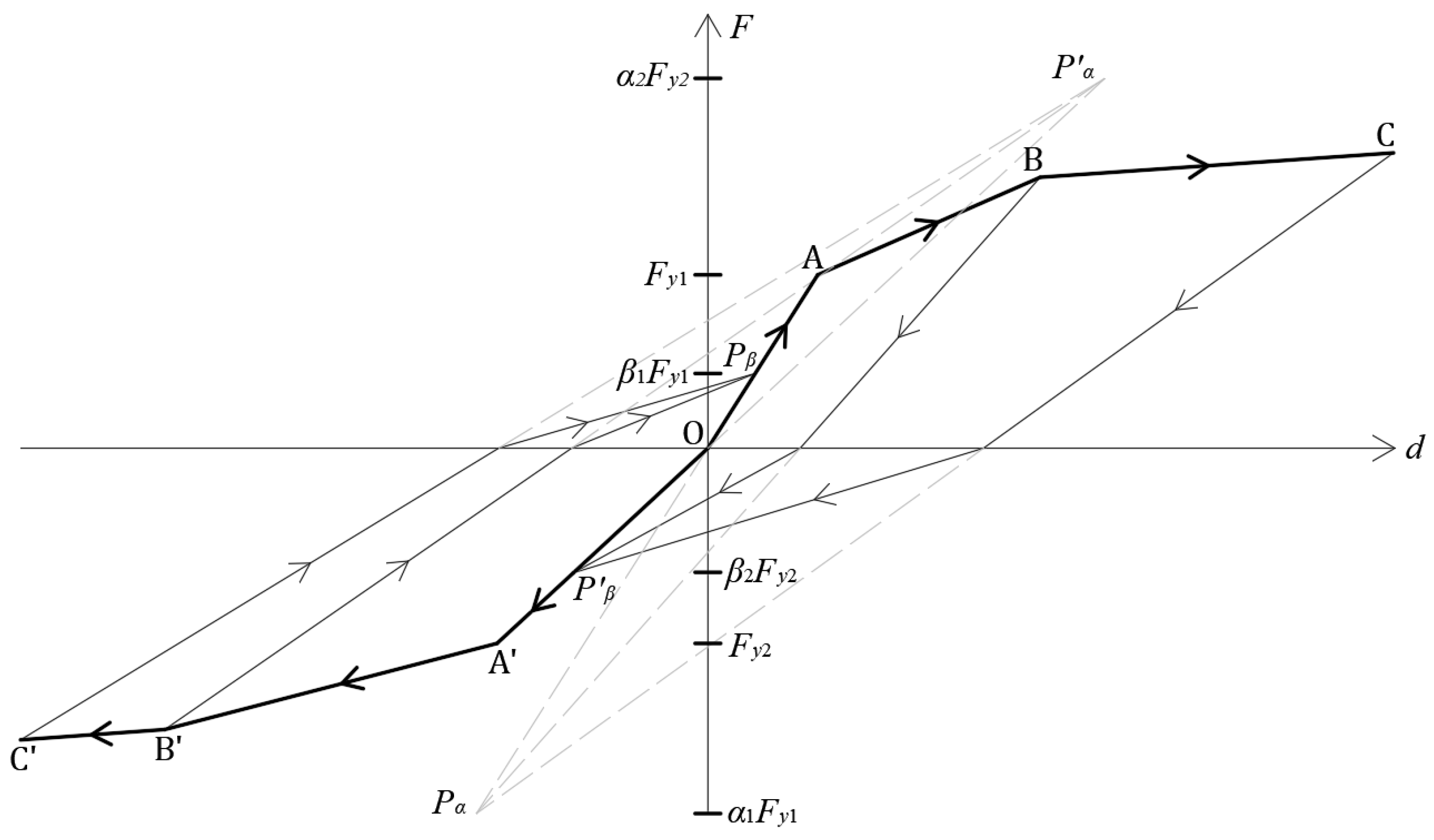
2. Modeling Assumptions
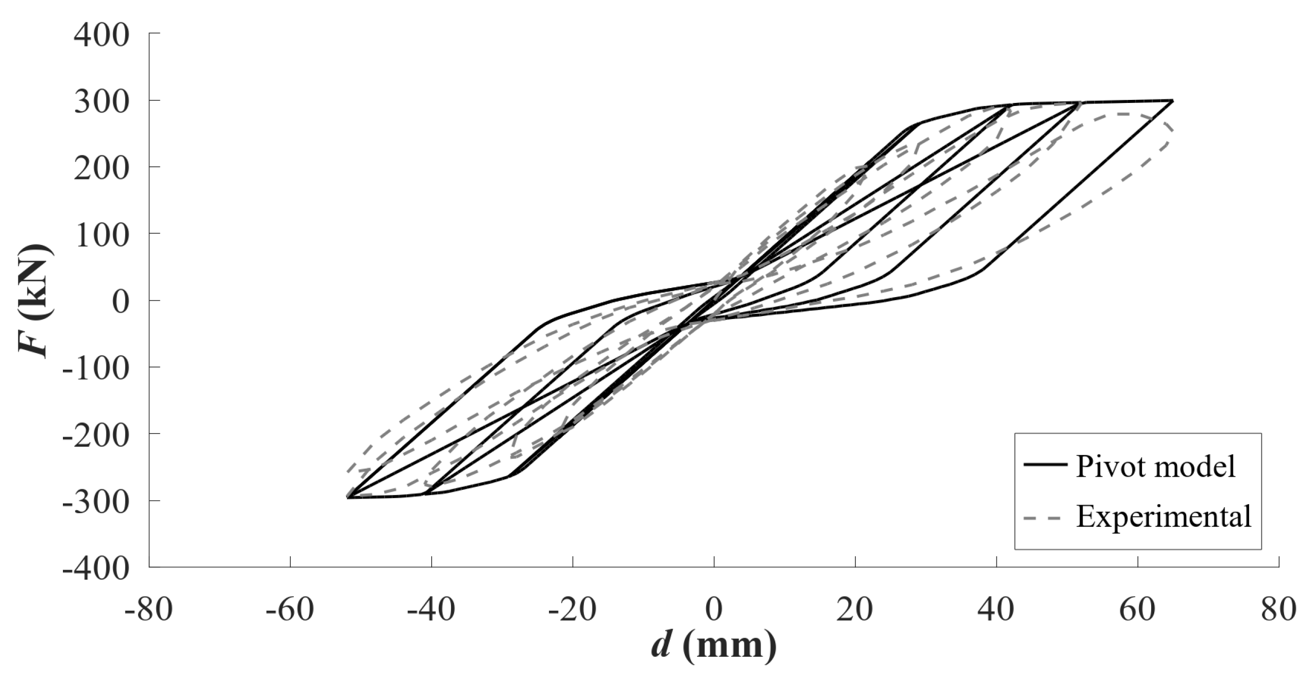
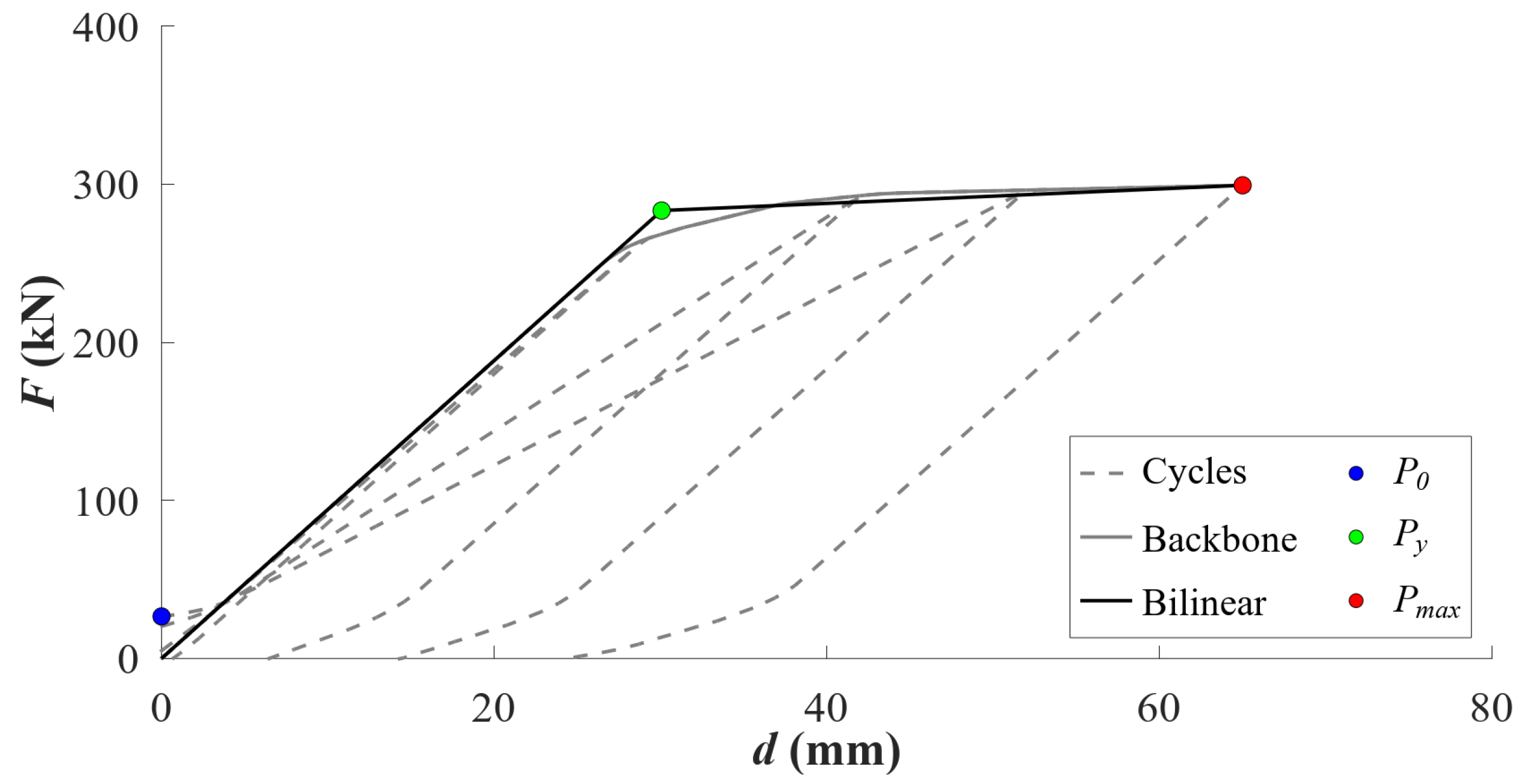
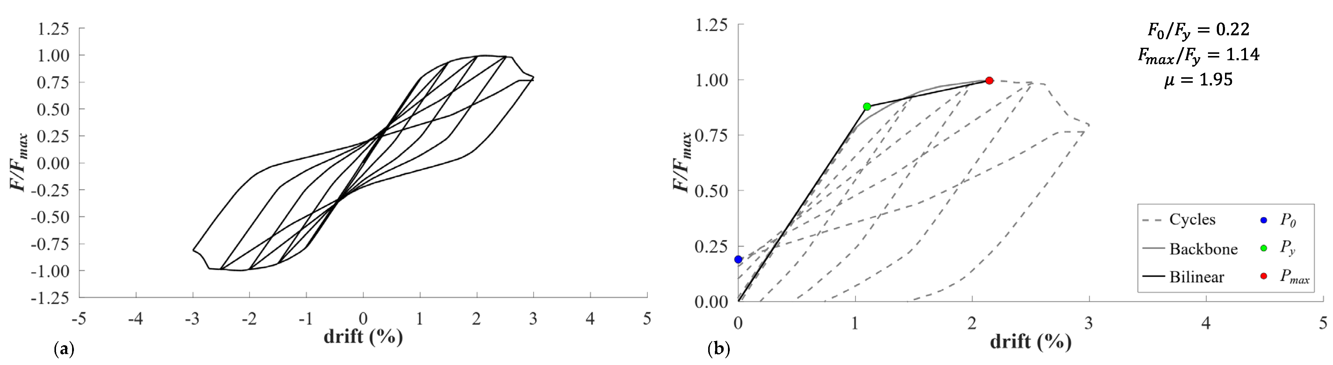
In this section, the modeling strategy adopted to perform the parametric study on the RC frames is illustrated. A fiber-based finite-length plastic hinge element is utilized for both the RC beams and the column elements. This element, pioneered by Scott and Fenves [13] and implemented in various software packages, such as OpenSees [14] and SeismoStruct [15], combines the accuracy of the distributed plasticity approaches with the computational advantages of the concentrated plasticity formulations.
In particular, the present work is based on the so-called fiber–hinge model (Fiber P-M2-M3) implemented in the structural analysis software SAP2000 [16]. This formulation describes the axial behavior of several axial fibers, each characterized by position, tributary area, and stress–strain curve, distributed along the cross section of the frame elements. The inelastic behavior is concentrated within a pre-specified length of the frame element, assumed here to be equal to the plastic hinge length L p l for reinforced concrete members calculated according to the Italian Building Code [17,18] expression:
L p l = 0.1 L V + 0.17 h + 0.24 d b l f y f c
where L v is the moment/shear ratio of the frame element, assumed to be approximately equal to h / 2 for columns ( h being the height of the cross section) and L / 3 for beams ( L being the element length), d b l is the average diameter of the reinforcing bars, and f y and f c are the steel yield strength and the concrete compressive strength, respectively (both expressed in MPa).
The axial force–deformation and biaxial moment–rotation relationships are given by the contribution of all the fibers, considering the above-specified hinge length. Axial force–biaxial bending interaction behavior, moment–rotation curve modifications, and plastic axial strain are automatically taken into account. With regard to the stress–strain relationships adopted for the various fibers, the non-linear elastic with plastic hardening stress–strain curve has been adopted for reinforcing the steel fibers, while the Mander et al. [19] stress–strain model has been adopted for concrete, by distinguishing between the confined model for concrete core and the unconfined model for concrete cover. For each section of the frame elements, the confined concrete ultimate strain ε c c u has been calculated according to the Italian Building Code [17,18] and Model Code 1990 [20] expressions:
ε c c u = ε c u + 0.1 α h α v ω s t
where ε c u is the unconfined concrete ultimate strain, assumed to be equal to 3.5‰, α h and α v represent the horizontal and vertical confinement efficiency factors, respectively, while ω s t is the mechanical volumetric shear–reinforcement ratio.
With regard to the hysteresis model governing the cyclic post-elastic response, the versatile pivot hysteresis model [11] has been adopted for both the beams and columns in order to incorporate the pinching effects ascribed to the weak transverse reinforcement and the poor construction details that might be observed in the existing RC structures. The pivot model is similar to the model proposed by Takeda et al. [8] for RC members but is equipped with additional input parameters that can be suitably calibrated to describe the possible pinching effects and degrading hysteretic loops. More specifically, in the pivot hysteresis model, the unloading and reloading tend to be directed toward specific points, called pivot points. Additional parameters required to calibrate the pivot model are α 1 , which regulates the unloading stiffness, determining the pivot point position for unloading from a positive force to zero; α 2 , analogous to α 1 but from a negative force; β 1 , ranging between 0 and 1, which regulates the pinching effects, determining the pivot point position for reloading from zero toward a positive force; β 2 , analogous to β 1 but toward a negative force; and η , which regulates the initial stiffness degradation following the cyclic plastic deformations. In the case of the section with symmetry properties (typically, RC columns), α 1 = α 2 = α and β 1 = β 2 = β . An example of the pivot hysteresis model along with the geometric interpretation of the above-introduced variables is shown in Figure 1.
Dowell et al. [11] introduced the model and provided contours for the evaluation of the α and β parameters for the circular RC columns, mainly used for bridge piers. The empirical relationships are also available in the literature. Sharma et al. [12] determined equations for the calculation of the α and β parameters specifically for rectangular RC columns, depending on the mechanical properties of the frame sections:
α = 0.170 k α + 0.415
β = 0.485 k β + 0.115
k α = p l / A L R  
k β = A L R 0.25 p s 0.2
where p l is the longitudinal reinforcement percentage; p s is the volumetric shear reinforcement percentage; and A L R is the ratio of the applied axial load on the column to the ultimate axial load capacity of the column. Regarding the evaluation of the η parameter, no specific relationships are provided. In Dowell et al. [11], it was reported that assuming a large value of the η parameter allowed an unloading stiffness to be obtained for small cycles, approximately equal to the unloading stiffness at the maximum displacement. In Sharma et al. [12], it was reported that because the analyses had been performed for only one cycle of loading, the effect of the η parameter was not considered.

3. Model Validation

The numerical study conducted here starts by simulating the seismic behavior of a real archetype prototype frame model tested in the laboratory. In particular, the one-bay, one-story RC frame tested by Lee et al. [21] has been considered, whose geometry and reinforcement configuration is shown in Figure 2. The RC frame is characterized by a clear span equal to 4.1 m and a net height of 3.075 m, assuming for the columns a fixed restraint at half of the foundation beam height, which is appropriate for capturing the initial stiffness of the RC frame in the first loading cycles (while avoiding explicitly modeling the bar slip and yield penetration phenomena). This prototype RC frame was tested in the laboratory [21], assuming an increasing cyclic horizontal loading protocol applied to the upper part of the frame, while no additional gravity load (apart from the self-weight) was applied.
The experimental load–displacement curve obtained experimentally has been simulated in a numerical model implemented in SAP2000 [16] by adopting the assumptions summarized in the previous section. According to the experimental source paper [21], concrete with a specified compressive strength of 21 MPa, an average compressive strength of 29.8 Mpa, and a modulus of elasticity of 24.8 GPa has been assumed, while reinforcing steel bars have been assumed to have average values of yield stress (455.9–497.6 MPa), tensile stress (580.5–656.6 MPa), and elongation (11.5–13.4%) dependent on the nominal size of the bar. The concrete cover, 3 cm thick in each section, has been assumed with no compressive strength. The pivot hysteresis model has been assumed for both the concrete and reinforcing steel, using the equations of Sharma et al. [12] for the α and β parameter calculations (cf. Equations (3)–(6)). Since no axial load has been applied and, consequently, A L R = 0 , α (a large value has been inputted), and β = 0.115 for both the beam and column members, the value of η has been assumed to be equal to 0. The fiber–hinge model P-M2-M3 has been adopted for both the beam and column members. Hinges have been applied at either end of the frame members. Cyclic pushover analysis has been performed through a sequence of pushover analyses, with each pushover analysis pushing the structure in the direction opposite to that of the preceding analysis and adopting the stiffness resulting from the end of the previous analysis, except for the first analysis where the initial stiffness has been used. Pushover analyses have been performed through a displacement–control load application at the beam–column joint, with a monitored displacement dependent on a specific cycle. A five-cycle loading protocol has been applied, with a monitored displacement of 22 mm for the first cycle, 29 mm for the second cycle, 42 mm (positive) and 41 mm (negative) for the third cycle, 52 mm for the fourth cycle, and 65 mm (positive) and 52 mm (negative) for the fifth and last cycle. The comparison between the load–displacement curve obtained from the cyclic pushover analysis performed on the numerical model and the experimental load–displacement curve is shown in Figure 3, while the main characteristic parameters of the curves, including maximum load (positive and negative), residual load (positive and negative) and global energy dissipated, are listed in Table 1.
As reported in Section 2, no specific relationships were given for the η parameter. In the pivot hysteresis model implemented in SAP2000 [16], η can assume values between 0 (minimum stiffness degradation) and 1 (maximum stiffness degradation). The comparison between the model load–displacement curves obtained with η = 0 and η = 1 is shown in Figure 4.
As can be seen from Figure 4, the two model curves are identical; therefore, it seems that the η parameter did not produce a significant effect on the load–displacement curve. This could be due to the number of cycles considered; the effects of the η parameter on the load–displacement curve with a greater number of cycles have not been investigated.
The present paper is focused on the determination of the seismic behavior of the RC frames through synthetic and practical indicators that can be used for design purposes. To this aim and to simplify the obtained cyclic behavior of the frame, first, the backbone branch enveloping the peaks for each cycle is obtained, then a bilinear curve with hardening idealization has been associated to this backbone load–displacement curve. The elastic branch of the bilinear curve passes through the origin and the point corresponding to a force value equal to 60% of the maximum force F m a x , while the hardening branch has a slope such that it passes through the point corresponding to the maximum force ( d m a x , F m a x ) and satisfies the energy equivalence condition (equal to the enclosed area) between the bilinear and backbone curves in the range 0 d m a x . The observation of the idealized bilinear curve has made it possible to identify three main characteristic points that are sufficient to describe not only the loading branch of the seismic response (backbone) but also the unloading branch and the associated recentering behavior. In particular, based on the backbone and the associated bilinear curves, it is possible to obtain different parameters, such as the yielding point P y = ( d y , F y ) , maximum point P m a x = ( d m a x , F m a x ) , and unloading residual force point P 0 = ( 0 , F 0 ) . From those parameters, it is possible to determine three synthetic parameters describing the cyclic response and recentering behavior of the RC frame, namely a “recentering index F 0 / F y , a “hardening index”  F m a x / F y , and a “ductility index”  μ = d m a x / d y . The bilinear curve with identification of the above-introduced characteristic points is illustrated in Figure 5, while the corresponding parameters are listed in Table 2.

4. Parametric Study

4.1. Selection of Parameter Ranges

To generalize the results for a range of practical reinforcement configurations and to provide some guidelines that can be useful to describe the seismic response and recentering behavior of the RC frames, a parametric study has been performed considering different values of A L R , p l , and p s . Based on the model defined in Section 3, different configurations of axial load and reinforcement details were analyzed within the following ranges:
  • A L R = (0.05; 0.20; 0.40; 0.60; 0.80);
  • p l = (1%; 2%; 3%; 4%);
  • p s = (0.40%; 0.80%; 1.20%; 1.60%).
The values selected for A L R cover almost the entire spectrum of possible values for RC frames, taking into account both weakly and heavily loaded configurations in relation to the compressive strength capacity of the frame columns. Similarly, the range selected for p l covers almost every possible configuration for the RC columns; for example, the Italian Building Code [17,18] sets the lower and upper bounds of longitudinal reinforcement ratios for the RC columns’ design equal to 1% and 4%, respectively. Finally, the range of p s depends on stirrup spacing and cross ties. Having in mind the RC columns with non-seismic construction details, such as stirrups with no additional cross ties and wide spacing, values in the order of 0.40% (lower bound) might be reasonable, whereas values in the order of 1.60% (upper bound) reflect the amounts of transverse reinforcement typically observed in the critical regions of the well-designed RC frames in the seismic area. Cyclic pushover analyses have been performed, as described in Section 3, applying a loading protocol with an increasing drift reaching up to F m a x or up to failure if it occurred at a lower drift. In the analyses, the appropriate A L R value has been obtained by applying forces to the columns at the beam–column joints. Considering all the combinations of the A L R , p l , and p s values in the above intervals, 80 scenarios have been obtained. The results are shown in terms of both the force–drift curves (where the forces are displayed in a normalized form as F / F m a x ) and 3D surface and contour plots of the three indexes F 0 / F y , F m a x / F y , and μ . It has been found that the behavior of the frame in terms of the cyclic response and recentering properties is very different depending on the combination of the A L R , p l , and p s values considered. Some representative examples are given in the following subsection and critically commented.

4.2. Results in Terms of Force–Drift Curves

The force–drift results obtained for A L R = 0.05 − p l = 4% − p s = 1.20% are reported in Figure 6a; in this case, the frame tends to exhibit a stable cyclic response with prominent pinching effects. Since the applied axial load is very low compared with the column compressive capacity, the frame exhibits high displacement capacity as well as good recentering capacity since the observed unloading residual force value is low, while the hardening behavior is moderate due to a high amount of longitudinal reinforcement. It follows that the frame is characterized by a low recentering index F 0 / F y and intermediate values of hardening and ductility indexes F m a x / F y and μ , respectively, as reported in Figure 6b.
The force–drift results obtained for A L R = 0.20 − p l = 4% − p s = 1.60% are illustrated in Figure 7a; also in this case, the frame tends to exhibit a stable cyclic response and significant pinching effects. The applied axial load is low compared with the column compressive capacity; therefore, the frame shows a high displacement capacity and good recentering behavior, although it is slightly lower than the case when A L R = 0.05, while the hardening behavior is high due to the high reinforcement percentage and the higher A L R value. It follows that the frame is characterized by a low recentering index F 0 / F y , a high hardening index F m a x / F y , and an intermediate ductility index μ , as illustrated in Figure 7b.
The force–drift results obtained for A L R = 0.40, p l = 3% and p s = 1.20% are illustrated in Figure 8a; in this case, the cyclic response is still stable, and the pinching effects are instead attenuated. Therefore, the frame presents a lower recentering capacity (than in the previous cases) since the observed unloading residual force value is higher. Since the applied axial load is moderate and close to the value corresponding to the maximum flexural strength, the frame shows a high displacement capacity and a moderate hardening behavior. It follows that the frame is characterized by a high F 0 / F y value, an intermediate F m a x / F y value, and a high μ value, as illustrated in Figure 8b.
The force–drift results obtained for A L R = 0.60, p l = 2%, and p s = 0.80% are illustrated in Figure 9a; in this case, the cyclic response becomes unstable, and the pinching effects are very attenuated. The recentering capacity is moderate since the observed unloading residual force is small, but since the applied axial load has reached a significant intensity, the frame shows a low displacement capacity, exhibiting a brittle failure occurring at a relatively low drift value. It follows that the frame is characterized by intermediate values of F 0 / F y , F m a x / F y , and μ , as depicted in Figure 9b.
Finally, the force–drift results obtained for A L R = 0.80, p l = 2% and p s = 1.20% are shown in Figure 10a. Although the graphs in this case are poorly visible because of the adoption of a consistent axis scale with the previous plots, it can be noted that the cyclic response is very unstable, and the pinching effects are almost null. Since the applied axial load has reached a very high intensity, the frame shows a negligible displacement capacity, reaching a brittle failure for a very low drift value. The hardening behavior and recentering capacity are evidently affected by the low drift value reached, as confirmed by the values of F 0 / F y , F m a x / F y , and μ , as shown in Figure 10b.

4.3. Three-Dimensional Surface and Contour Plots of Synthetic Behavioral Indexes

Based on the entire set of results for the 80 cases of the parametric study, 3D surfaces describing the variation of F 0 / F y , F m a x / F y , and μ depending on A L R , p l , and p s have been obtained by cubic interpolation of the discrete values obtained. These 3D surfaces are useful for synthetically describing the trends of the seismic response and recentering capacity of the analyzed set of the RC frames based on the loading and reinforcement configuration. From the 3D surfaces derived above, we also construct contours for the evaluation of F 0 / F y , F m a x / F y , and μ as a function of A L R and p l for a given value of p s , which can be used for practical design purposes, as illustrated in the sequel to this paper. It is worth noting that the F 0 values for the cases with A L R ≥ 0.60, affected by a significant variation between the cycles and asymmetric cyclic behavior, as observed in the previous examples, is assumed as the average value of F 0 + and F 0 . For the cases with A L R < 0.60, this averaging process is not necessary since the trend of the cycles is regular and symmetrical; consequently, the variations mentioned above are negligible. Therefore, in these cases, only the positive value F 0 + = F 0 has been reported. The 3D surfaces and related contour plots mentioned above are shown and commented on below.
By observing the trends depicted in Figure 11, Figure 12, Figure 13, Figure 14, Figure 15 and Figure 16, the following general considerations can be drawn:
(1)
The recentering index is much more sensitive to the A L R than to the longitudinal and transverse reinforcement. In particular, for given p l and p s values, variations up to 100% of the F 0 / F y parameter are observed by spanning the range of A L R investigated. Such variations are more marked for low amounts of steel reinforcement (see, e.g., the variability of F 0 / F y corresponding to p s = 0.40 % and p l 1 1.25 % shown in the left part of Figure 11) and tend to diminish for higher amounts of steel reinforcement. The peak values of F 0 / F y (poorest recentering behavior) are generally observed in the range of A L R = 0.35 0.40 , which characterizes most of the RC column configurations encountered in the existing buildings. The sensitivity of F 0 / F y with respect to p l is relatively modest, while the presence of higher amounts of transverse reinforcement slightly increases the recentering index. It is worth noting that these trends consistently reflect, at a structural (macroscopic) scale, the empirical relationships expressed at the material (microscopic) level by the calibration parameters of the pivot model derived by Sharma et al. [12] and reported in Equations (3)–(6).
(2)
The hardening index F m a x / F y is instead more correlated (than F 0 / F y ) with the longitudinal reinforcement since, as reasonably expected, higher values of p l lead to an increase in the overall flexural capacity of the RC frame. The peak values of the F m a x / F y parameter are identified in a range of the A L R value that somehow depends on the transverse reinforcement, i.e., it is close to A L R = 0.3 0.4 for lower amounts of transverse reinforcement ( p s = 0.40 % ) and close to A L R = 0.5 0.6 for higher amounts ( p s = 1.60 % ). This indicates that there is a reciprocal influence between the hardening behavior and the loading condition in terms of axial load, as reasonably expected.
(3)
The deformation capacity of the RC frame is expressed in this work by the ductility index μ . As reasonably expected, higher values of μ are observed for lower value A L R scenarios, which correspond to the flexural failures being dominated by the steel reinforcement that is largely yielded due to the high value of the ultimate curvature (resulting from a small value of neutral axis depth). Moreover, the increase in the transverse reinforcement leads to higher confinement effects in the RC columns, which, in turn, are beneficial in terms of ductility. This is reflected in the larger values of μ observed for p s = 1.20 1.60 % compared with those obtained for p s = 0.40 0.80 % for comparable values of A L R . The influence of p l on μ is rather negligible in the entire range of the parameters explored, apart from very low values of A L R (0.05–0.15), where higher amounts of longitudinal reinforcement may generate more brittle failure modes associated with lower values of μ .
Figure 11. Three-dimensional surface and contour plots of the recentering index F 0 / F y for p s = 0.40 % and 0.80 % .
Applsci 13 08549 g011
Figure 12. Three-dimensional surface and contour plots of the recentering index F 0 / F y for p s = 1.20 % and 1.60 % .
Applsci 13 08549 g012
Figure 13. Three-dimensional surface and contour plots of the hardening index F m a x / F y for p s = 0.40 % and 0.80 % .
Applsci 13 08549 g013
Figure 14. Three-dimensional surface and contour plots of the hardening index F m a x / F y for p s = 1.20 % and 1.60 % .
Applsci 13 08549 g014
Figure 15. Three-dimensional surface and contour plots of the ductility index μ for p s = 0.40 % and 0.80 % .
Applsci 13 08549 g015
Figure 16. Three-dimensional surface and contour plots of the ductility index μ for p s = 1.20 % and 1.60 % .
Applsci 13 08549 g016
The usefulness of the constructed 3D surface and contour plots in predicting the seismic response and recentering behavior of the RC frames will be demonstrated in the following section by means of a numerical case study on a multi-story existing RC frame designed only for gravity loads.

5. Nonlinear Time History Analysis on a Multi-Story RC Building

This section is aimed at demonstrating the usefulness of the results illustrated in the parametric study for describing the cyclic behavior of the RC frames. To this aim, an eight-story RC frame with non-seismic details, reported in Masi and Vona [22] and designed in accordance with the 1972 Italian Building Code [23], was analyzed. This represents an archetypal building, representative of the substandard RC frames built in the 1960s–1970s in Italy. The plan view and front view, along with the section details and reinforcement arrangement, are depicted in Figure 17. The material parameters considered for calibrating the nonlinear material behavior via fiber–hinge elements in the RC frame, directly taken from the reference paper [22], are listed in Table 3. Considering the regularity in the plan and in the elevation, nonlinear time history analyses (NTHAs) were carried out on a simplified planar model of the internal frame (highlighted with a dashed red rectangle in Figure 17), as per EC8 §4.2.3 [24].
From the analysis for gravitational loads, the values of the axial load acting on the columns (prior to the application of the seismic loads) were obtained based on which values of A L R were calculated for each column. The longitudinal reinforcement percentage p l and volumetric shear reinforcement percentage p s were evaluated from the reinforcement arrangement details reported above. Once the A L R , p l , and p s values were determined, the pivot hysteresis model was calibrated for each structural member according to the equations of Sharma et al. [8]. As dynamic input, a sinusoidal acceleration of period T = 0.64 s, amplitude a g = 0.25 g (selected to reach a sufficiently high story drift in all story levels, so as to describe the post-elastic cyclic behavior), and the number of cycles n = 10 (to investigate the recentering behavior after the repetition of multiple cycles) was applied at the base of the frame. It is worth noting that in the case of a multi-story building, the seismic response and recentering behavior of each story level j could be described in terms of the inter-story drift δ j and story shear force V j ; hence, the characteristic points P 0 , P y , and P m a x were identified in the V / V m a x δ plane (the shear force was normalized with respect to its maximum value for comparison purposes among the story levels). Consequently, the previously defined indexes for the j t h story level were calculated: recentering index V 0 , j / V y , j ; hardening index V m a x , j / V y , j ; and ductility index μ = δ m a x , j / d y , j . Based on these considerations, the inter-story drift versus the normalized story shear force diagrams and the related bilinear idealized curve for story levels 2, 3, 7, and 8, along with related characteristic points and behavioral indexes, are shown in Figure 18, Figure 19, Figure 20 and Figure 21. It is worth noting that, for the sake of brevity, only four of the eight story levels are considered here to illustrate some representative results associated with the different A L R values.
It is clearly seen that the shape of the hysteretic loops is different (in terms of pinching, ductility, and hardening factors) depending on the story level considered. This is ascribed to the different mechanical parameters A L R , p l , and p s characterizing each story level. Considering the actual values of A L R i , p l , i , and p s , i at each storey level i, we can compare the numerical results from the NTHAs with the predictions from the parametric study for the consistent combination of the parameters. To check the reliability and generality of the contour plots constructed in the previous section, the characteristic behavioral indexes F 0 / F y , F m a x / F y , and μ are compared with those identified from the inter-story drift versus the normalized story shear force graphs at each story level.
All four of the representative story levels considered have an identical volumetric shear reinforcement percentage p s (roughly equal to 0.3%); therefore, a reference has been made to the contours pertinent to p s = 0.40%. Different A L R and p l values are associated with each story level; in particular, the longitudinal reinforcement percentage p l for story level 2 is equal to 0.68%, while for story levels 3, 7, and 8, p l is equal to 0.50%. Consequently, a reference has been made to the minimum value considered in the parametric study, that is, p l = 1%. Regarding A L R , it should be noted that the four columns of each story level do not have the same axial load intensity. In particular, for the gravity loads, the frame is symmetrical and uniformly loaded, which makes it reasonable to assume that the internal columns have twice the axial load as compared with the external columns. However, for practical purposes, a single average value of A L R per story level has been defined to facilitate the use of the contour and surface plots of the parametric study. Such an average A L R value is equal to 0.40 for the story level 2, 0.34 for the story level 3, 0.10 for the story level 7, and 0.05 for the story level 8. Once the values of A L R , p l , and p s had been determined, these were used to estimate the three behavioral indexes from the contours (shown in Figure 22), and then they were compared with the actual behavioral indexes evaluated from the hysteretic loops listed in Figure 23.
Based on the comparison reported in Figure 23, we note that there is an excellent agreement between the estimates of the behavioral indexes from the contour plots of the parametric study (carried out on a single-story prototype RC frame) and those from the NTHAs on a multi-story building with different geometric and mechanical characteristics. This comparison emphasizes the usefulness of the contour plots/surface plots drawn in Section 4 in anticipating the overall cyclic behavior of a generic RC building, depending on the actual mechanical parameters of the RC sections at each story level.
The authors believe that these behavioral indexes are important parameters that can be used in practical design contexts. As an example, the recentering index is strictly related to the ability of each story level to return to its original position at the end of the earthquake shaking. To prove this, the NTHAs have been repeated by adding at the end of the 10 cycles a zero-acceleration segment of duration 20 s, thus making it possible to investigate the free vibration response of the structure. This augmented time history is purposely considered to check whether the RC frame is able to return to its original configuration or has accumulated a permanent residual displacement at the end of the seismic event due to its poor recentering attitude. The inter-story drift time histories obtained for story level 3 and 8 are shown below.
As can be seen from Figure 24, in floor 3, a permanent residual drift equal to 0.12% has been accumulated, whereas negligible residual displacement was noted in floor 8. This different recentering attitude is indeed ascribed to the different value of the recentering index associated with the two considered story levels (0.28 for floor 3 and 0.13 for floor 8), which directly influences the value of the recentering force at zero displacement, as explained in Section 3. It is worth noting that if one considers more severe seismic excitations, a longer duration of the earthquake event, or a sequence of foreshocks, mainshocks, and aftershocks, the value of the residual drift could be even greater. In cases like these, a retrofitting strategy could be planned to avoid an excessive accumulation of the permanent residual drift in the RC frame in those specific story levels associated with poor recentering ability. As an example, one could implement devices capable of improving the recentering behavior of the RC frame, such as self-recentering dampers [25]. The usefulness of the parametric study discussed in this work for designing self-centering dissipative devices for retrofitting purposes is beyond the scope of this article and represents the object of an ongoing research study, whose details will be published in a forthcoming paper.

6. Conclusions

In this paper, the seismic response and recentering behavior of RC frames has been analyzed numerically in order to construct novel design abacuses in the form of practical 3D surface/contour plots. These plots were useful to anticipate the inelastic response of a building structure based on the actual mechanical parameters of the RC sections at each story level. Cyclic pushover analysis has been performed on a wide spectrum of RC frames having different axial load levels and reinforcing details within a parametric study including 80 scenarios, covering a reasonable set of configurations that can be encountered in the existing RC-framed structures. A fiber–hinge formulation combined with the versatile pivot hysteresis model has been adopted, validated against experimental findings, and used in the cyclic pushover analyses of the parametric study.
The main results of this work can be summarized as follows:
1.
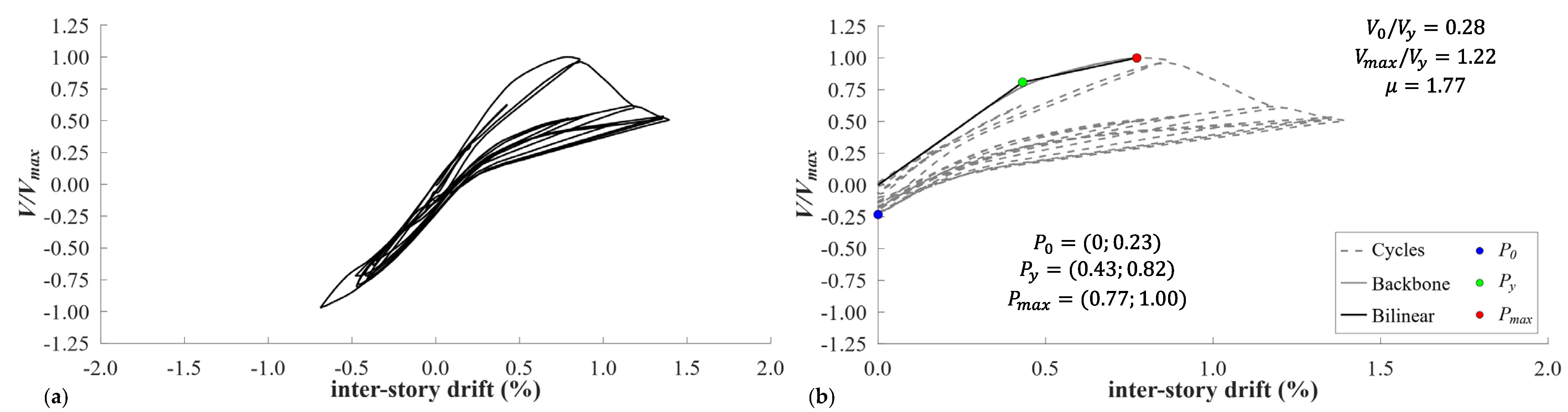
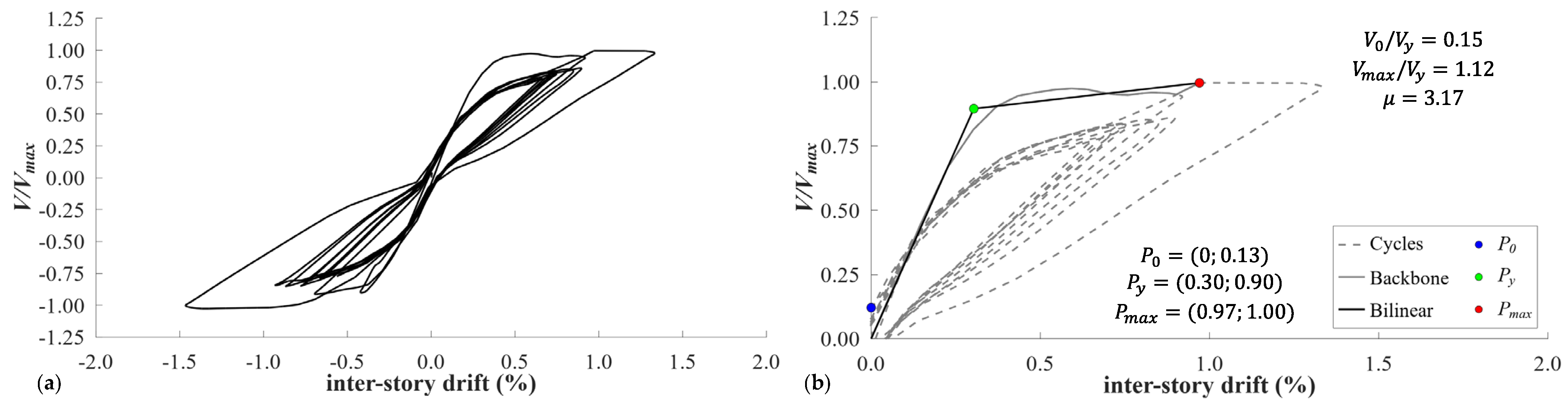
The cyclic behavior of the RC frames has been described by a backbone branch enveloping the peaks for each cycle of the cyclic pushover analysis and then idealized through a bilinear curve with hardening. The unloading residual force has also been incorporated in the parametric study to investigate the recentering behavior of the RC frames related to the possible pinching effects of the existing RC structures with poor construction details.
2.
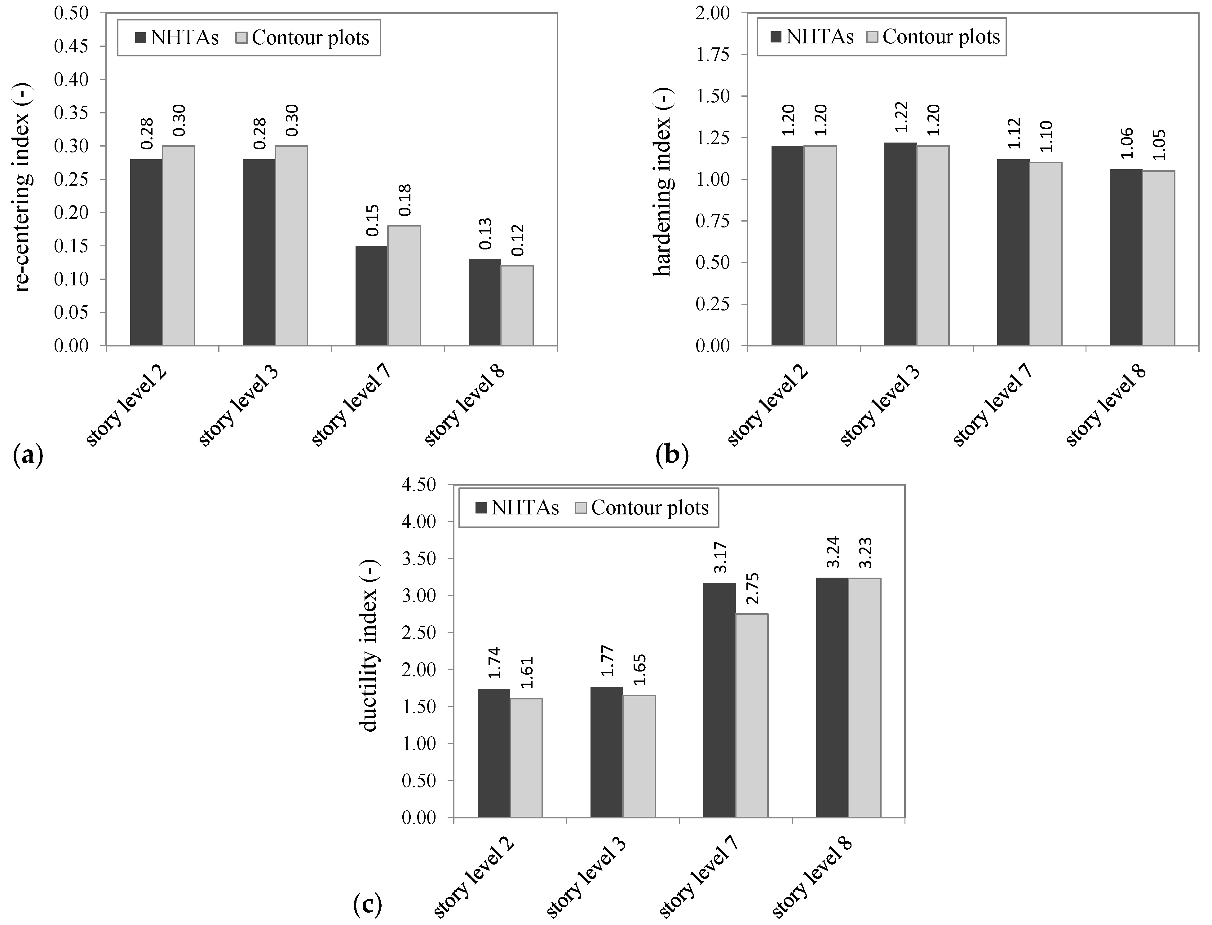
The inelastic behavior of the RC frames can be described synthetically by means of three behavioral indexes, namely a recentering index, a hardening index, and a ductility index, whose trends have been described in this work through 3D surface and contour plots. These indexes were able to describe the backbone as well as the hysteretic behavior of the RC frame as a whole, depending on the axial load ratio A L R , longitudinal reinforcement percentage p s , and volumetric transverse reinforcement percentage p s of each story level.
3.
The recentering index was much more sensitive to the A L R than to the longitudinal and transverse reinforcement. The variations were more marked for low amounts of steel reinforcement and tended to diminish for higher amounts of steel reinforcement. The poorest recentering behavior was generally observed in a range of A L R = 0.35 0.40 , which characterized most of the RC column configurations encountered in existing buildings.
4.
The hardening index was highly correlated with the longitudinal reinforcement since, as reasonably expected, higher values of p l led to an increase in the overall flexural capacity of the RC frame. A reciprocal influence between the hardening behavior and the loading condition in terms of axial load has been detected in the analyses, as the peak values of the hardening index were identified in a range of A L R values that somehow depended on the transverse reinforcement.
5.
The deformation capacity of the RC frame, expressed by the ductility index, was higher for lower A L R scenarios. Moreover, the increase in the transverse reinforcement led to higher confinement effects in the RC columns, and this trend was consistently reflected in the numerical results obtained in the parametric study.
6.
The estimates of the behavioral indexes reported in the contour plots of the parametric study were compared with the actual values obtained from the NTHAs on an eight-story building representative of the substandard RC frames built in the 1960s–1970s in Italy. The excellent agreement between the two sets of results has emphasized the usefulness of the constructed 3D surface and contour plots in predicting the seismic response and recentering behavior of a generic RC building, depending on the actual mechanical parameters of the RC sections at each story level, thus highlighting the importance of this parametric study for practical design purposes.

Author Contributions

Conceptualization, D.D.D., E.G. and A.G.; methodology, D.D.D., E.G. and A.G.; software, A.G; validation, E.G. and A.G.; formal analysis, D.D.D., E.G. and A.G.; investigation, D.D.D. and E.G.; data curation, D.D.D., E.G. and A.G.; writing—original draft preparation, D.D.D. and A.G.; writing—review and editing, D.D.D. and E.G.; visualization, D.D.D. and E.G.; supervision, D.D.D. and E.G. All authors have read and agreed to the published version of the manuscript.

Funding

This research received no external funding.

Institutional Review Board Statement

Not applicable.

Informed Consent Statement

Not applicable.

Data Availability Statement

The data used to support the findings of this study are available upon reasonable request.

Conflicts of Interest

The authors declare no conflict of interest.

References

  1. Gurbuz, T.; Cengiz, A.; Kolemenoglu, S.; Demir, C.; Ilki, A. Damages and failures of structures in Izmir (Turkey) during the October 30, 2020 Aegean Sea earthquake. J. Earthq. Eng. 2023, 27, 1565–1606. [Google Scholar] [CrossRef]
  2. Aynur, S.; Atalay, H.M. Comparative analysis of existing reinforced concrete buildings damaged at different levels during past earthquakes using rapid assessment methods. Struct. Eng. Mech. 2023, 85, 793. [Google Scholar]
  3. Monteiro, R.; Araújo, M.; Delgado, R.; Marques, M. Modeling considerations in seismic assessment of RC bridges using state-of-practice structural analysis software tools. Front. Struct. Civ. Eng. 2018, 12, 109–124. [Google Scholar] [CrossRef]
  4. Salgado, R.A.; Guner, S. A comparative study on nonlinear models for performance-based earthquake engineering. Eng. Struct. 2018, 172, 382–391. [Google Scholar] [CrossRef]
  5. Bruschi, E.; Calvi, P.M.; Quaglini, V. Concentrated plasticity modelling of RC frames in time-history analyses. Eng. Struct. 2021, 243, 112716. [Google Scholar] [CrossRef]
  6. Mazza, F. A distributed plasticity model to simulate the biaxial behaviour in the nonlinear analysis of spatial framed structures. Comput. Struct. 2014, 135, 141–154. [Google Scholar] [CrossRef]
  7. De Domenico, D.; Messina, D.; Recupero, A. Seismic vulnerability assessment of reinforced concrete bridge piers with corroded bars. Struct. Concr. 2023, 24, 56–83. [Google Scholar] [CrossRef]
  8. Takeda, T.; Sozen, M.A.; Nielsen, N.N. Reinforced concrete response to simulated earthquakes. J. Struct. Div. 1970, 96, 2557–2573. [Google Scholar] [CrossRef]
  9. Sezen, H.; Chowdhury, T. Hysteretic model for reinforced concrete columns including the effect of shear and axial load failure. J. Struct. Eng. 2009, 135, 139–146. [Google Scholar] [CrossRef]
  10. Jiang, Y.; Saiidi, M. Four-spring element for cyclic response of R/C columns. J. Struct. Eng. 1990, 116, 1018–1029. [Google Scholar] [CrossRef]
  11. Dowell, R.K.; Seible, F.; Wilson, E.L. Pivot Hysteresis Model for Reinforced Concrete Members. ACI Struct. J. 1998, 95, 607–617. [Google Scholar]
  12. Sharma, A.; Eligehausen, R.; Reddy, G.R. Pivot Hysteresis Model Parameters for Reinforced Concrete Columns, Joints, and Structures. ACI Struct. J. 2013, 110, 217–227. [Google Scholar]
  13. Scott, M.H.; Fenves, G.L. Plastic hinge integration methods for force-based beam–column elements. J. Struct Eng. 2006, 132, 244–252. [Google Scholar] [CrossRef]
  14. Mazzoni, S.; McKenna, F.; Scott, M.H.; Fenves, G.L. OpenSees command language manual. Pac. Earthq. Eng. Res. (PEER) Cent. 2006, 264, 137–158. [Google Scholar]
  15. Seismosoft. “SeismoStruct—A Computer Program for Static and Dynamic Nonlinear Analysis of Framed Structures”. 2023. Available online: http://www.seismosoft.com (accessed on 23 May 2023).
  16. Computers and Structures, Inc. (CSI). Analysis Reference Manual for SAP2000; CSI: Berkeley, CA, USA, 2022. [Google Scholar]
  17. Consiglio Superiore dei Lavori Pubblici (CSLLPP). Aggiornamento delle Norme Tecniche per le Costruzioni; CSLLPP: Rome, Italy, 2018.
  18. Consiglio Superiore dei Lavori Pubblici (CSLLPP). Istruzioni per L’applicazione Dell’aggiornamento delle Norme Tecniche per le Costruzioni; CSLLPP: Rome, Italy, 2019.
  19. Mander, J.B.; Priestley, M.J.N.; Park, R. Theoretical Stress-Strain Model for Confined Concrete. J. Struct. Eng. 1988, 114, 1804–1826. [Google Scholar] [CrossRef] [Green Version]
  20. Comité Euro-International du Béton (CEB). CEB-FIP Model Code 1990: Design Code; CEB T. Telford: London, UK, 1993. [Google Scholar]
  21. Lee, C.-H.; Ryu, J.; Kim, D.-H.; Ju, Y.K. Improving seismic performance of non-ductile reinforced concrete frames through the combined behavior of friction and metallic dampers. Eng. Struct. 2018, 172, 304–320. [Google Scholar] [CrossRef]
  22. Masi, A.; Vona, M. Vulnerability assessment of gravity-load designed RC buildings: Evaluation of seismic capacity through non-linear dynamic analyses. Eng. Struct. 2012, 45, 257–269. [Google Scholar] [CrossRef]
  23. Consiglio Superiore dei Lavori Pubblici (CSLLPP). Norme Tecniche Alle Quali Devono Uniformarsi le Costruzioni in Conglomerato Cementizio, Normale e Precompresso ed a Struttura Metallica; CSLLPP: Rome, Italy, 1972.
  24. EN1998-1:2004; Eurocode 8: Design of Structures for Earthquake Resistance. General Rules, Seismic Actions and Rules for Buildings. CEN (European Committee for Standardisation: Brussels, Belgium, 2004.
  25. Bagheri, H.; Hashemi, A.; Yousef-Beik, S.M.M.; Zarnani, P.; Quenneville, P. New self-centering tension-only brace using resilient slip-friction joint: Experimental tests and numerical analysis. J. Struct. Eng. 2020, 146, 04020219. [Google Scholar] [CrossRef]
Figure 1. Example of pivot hysteresis model.
Applsci 13 08549 g001
Figure 2. Geometric and reinforcement details of the RC frame simulated in this study.
Applsci 13 08549 g002
Figure 3. Comparison of load–displacement curves between experimental and pivot models.
Applsci 13 08549 g003
Figure 4. Comparison between model load–displacement curves with η = 0 and η = 1 .
Applsci 13 08549 g004
Figure 5. Bilinear curve obtained for the prototype RC frame.
Applsci 13 08549 g005
Figure 6. Force–drift curve (a) and bilinear idealization (b) for A L R = 0.05 − p l   = 4% − p s = 1.20%.
Applsci 13 08549 g006
Figure 7. Force–drift curve (a) and bilinear idealization (b) for A L R = 0.20 − p l   = 4% − p s = 1.60%.
Applsci 13 08549 g007
Figure 8. Force–drift curve (a) and bilinear idealization (b) for A L R = 0.40 − p l   = 3% − p s = 1.20%.
Applsci 13 08549 g008
Figure 9. Force–drift curve (a) and bilinear idealization (b) for A L R = 0.60 − p l   = 2% − p s = 0.80%.
Applsci 13 08549 g009
Figure 10. Force–drift curve (a) and bilinear idealization (b) for A L R = 0.80 − p l   = 2% − p s = 1.20%.
Applsci 13 08549 g010
Figure 17. RC frame selected for the time history analysis, taken from Masi and Vona [22].
Applsci 13 08549 g017
Figure 18. Inter-story drift versus normalized story shear force (a) and bilinear idealization (b) for story level 2.
Applsci 13 08549 g018
Figure 19. Inter-story drift versus normalized story shear force (a) and bilinear idealization (b) for story level 3.
Applsci 13 08549 g019
Figure 20. Inter-story drift versus normalized story shear force (a) and bilinear idealization (b) for story level 7.
Applsci 13 08549 g020
Figure 21. Inter-story drift versus normalized story shear force (a) and bilinear idealization (b) for story level 8.
Applsci 13 08549 g021
Figure 22. Behavioral indexes identified from the contour plots relative to p s = 0.40 % .
Applsci 13 08549 g022
Figure 23. Comparison between behavioral indexes obtained from NTHAs and from the contour plots of the parametric study: (a) recentering index; (b) hardening index; (c) ductility index.
Applsci 13 08549 g023
Figure 24. Inter-story drift time histories obtained for floors 3 and 8.
Applsci 13 08549 g024
Table 1. Maximum strength F m a x (positive and negative), maximum strength at zero displacement F 0 (positive and negative), and dissipated energy E d i s s values related to experimental and numerical model curves.
ExperimentNumerical ModelRelative Error (%)
F m a x (+) (kN)300.6299.30.4
F m a x (−) (kN)294.0295.90.6
F 0 (+) (kN)26.726.41.1
F 0 (−) (kN)30.430.11.0
E d i s s (kJ)27.226.62.2
Table 2. Characteristic parameters obtained for the prototype RC frame.
Prototype RC FramePoint d (mm) F (kN)
F 0 / F y F m a x / F y μ P 0 026.4
(−)(−)(−) P y 30283.3
0.091.062.17 P m a x 65299.3
Table 3. Material properties of the RC frame in Figure 17.
MaterialParameterValue
Concrete C20/25Cubic characteristic strength R c k = 25 MPa
Cylindrical characteristic strength f c k = 20 MPa
Cylindrical average strength f c m = 28 MPa
Ultimate deformation ε c u = 0.5%
Reinforcing steel A38Characteristic yielding strength f y k = 380 MPa
Average yielding strength f y m = 400 MPa
Ultimate deformation ε s u = 2.0%
Disclaimer/Publisher’s Note: The statements, opinions and data contained in all publications are solely those of the individual author(s) and contributor(s) and not of MDPI and/or the editor(s). MDPI and/or the editor(s) disclaim responsibility for any injury to people or property resulting from any ideas, methods, instructions or products referred to in the content.

