Two Revised Deep Neural Networks and Their Applications in Quantitative Analysis Based on Near-Infrared Spectroscopy

Abstract

Small data sets make developing calibration models using deep neural networks difficult because it is easy to overfit the system. We developed two deep neural network architectures by revising two existing network architectures: the U-Net and the attention mechanism. The major changes were to use 1D convolutional layers to replace the fully connected layers. We also designed and combined average pooling and maximum pooling in our revised networks, respectively. We applied these revised network architectures to three publicly available data sets and the resulting calibration models can generate acceptable results for general quantitative analysis. It also generated rather good results for data sets that concern calibration transfer. It demonstrates that constructing network architectures by properly revising existing successful network architectures may provide additional choices in the exploration of the application of deep neural network in analytical chemistry.

1. Introduction

Near-infrared spectroscopy (NIR) continues to be a developing analytical detection technique, and it is also one of the most effective means for qualitative, quantitative and structural analysis of organic matter. NIR combined with chemometrics and computer technology is fast, highly accuracy, and has low analysis costs. It can be applied to the simultaneous analysis of multiple components. Now, NIR techniques are widely used in medicine, food quality, industry, pharmaceuticals, and other fields [1,2]. For example, Shadrin et al. [3] proposed a method to analyze the different stages of apple tree disease. They found the best spectral bands to detect a specific disease and distinguish it from other diseases and healthy trees. Guo et al. [4] used NIR spectroscopy to analyze the contents of apple watercore and soluble solid to detect apple quality.

However, NIR techniques usually require a data set large enough to obtain good results. The data sets contain typical NIR spectra and the amount of the target species, which are used as reference samples. Calibration models are established using chemometric methods and then used to provide quantitative analysis of the target species from the samples [5]. The size of the reference samples has a large influence on the quality of the calibration model.

One of those chemometrics methods, the deep neural network (DNN), has some obvious advantages over traditional chemometric methods. DNNs can automatically extract features from spectral data [6,7] to better capture their nonlinear characteristics. Therefore, DNNs have strong, nonlinear modeling ability and can learn complex nonlinear relationships in spectral data. DNN is also suitable for processing high-dimensional data, which effectively reduces computational complexity through a series of operations such as convolution and parameter sharing. Most importantly, DNNs also have the ability to generalize the calibration, improving the generalization performance of models through data augmentation and end-to-end learning.

In recent years, many researchers have tried to use DNNs in analytical chemistry. Zeng et al. [8] reported a pattern recognition method using NIR spectroscopy for qualitative food analysis using a convolutional neural network architecture. Qu et al. [9] presented a DNN applied to nuclear magnetic resonance spectra using relatively small data sets. Gabrieli et al. [10] established a DNN classifier on an open source platform. By introducing users’ labeling of their data set, they developed a machine learning model for the automatic assessment of the quality of NIR signals. Rankine et al. [11] studied a deep neural network for fast prediction of X-ray absorption spectra, which can estimate the X-ray absorption spectra of near-edge structures of matter in a very short time without the need for geometric information about the local environment at the absorption location. Le [12] used a deep-learning stacked sparse autoencoder (SSAE) method to extract advanced features of NIR spectra and used an affine transformation (AT) and an extreme learning machine (ELM) to build prediction models. Gan and Luo [13] constructed the simplest possible DNN architecture. They showed that applying convolutional layers instead of fully connected layers was a good strategy to overcome the overfitting problem of small data sets.

In recent work, we followed our previous approach of simplicity in constructing DNN architectures, but the focus was on revising two existing well-known network architectures, the U-Net [14] and the attention mechanism [15]. The former was implemented for image segmentation while the latter was developed for sequence modeling and transduction problems. Guo et al. [16] applied a one-dimensional U-Net to remove artifacts from infrared spectra of complex samples. Wang et al. [17] applied the multiple-head self-attention mechanism to improve the representation and classification performance of this model. However, the applications of the two network architectures in quantitative analysis has not yet been applied to NIR spectral data. We modified the two networks by using 1D convolutions to replace the 2D ones. We also removed fully connected layers. Some additional changes were made to improve the performance of the revised networks. The method was tested by applying our revised networks to the quantitative analysis of near-infrared (NIR) spectral data.

The organization of this paper is as follows: (1) In the Section 2, we first discuss the data information. Then, we discuss the revising of the two networks in detail. Finally, we include a simple discussion of the hyperparameters. (2) In the Section 3, we present the results of applying the revised networks to three standard testing data sets. (3) In the Conclusion, we emphasize the reasons for the success of this work.

2. Materials and Methods

2.1. Data

The data sets are the same as our previous work [13]. The data sets have been widely applied to test the newly developed chemometric method. The details of the training sets, validation sets, and test sets are presented in

Table 1. The classifications of three data sets.

Data Set	Total Samples	Training Set	Validation Set	Test Set	Features 1
CGL	231	139	46	46	116
IDRC-2002 set 1	655	391	131	131	281
IDRC-2002 set 2	—	—	—	655	281
IDRC-2016 A1	248	248	—	—	740
IDRC-2016 A2	248	—	—	248	740
IDRC-2016 A3	248	—	—	248	740
IDRC-2016 B1	646	—	—	646	740
IDRC-2016 B2	248	—	—	248	740
IDRC-2016 B3	248	—	—	248	740
IDRC-2016 T	248	—	248	—	740
IDRC-2016 V	248	—	—	248	740

¹ These values are the numbers of measurement wavelength.

. The CGL data sets were downloaded from https://eigenvector.com/resources/data-sets/(access 6 June 2023). The data sets contain the NIR spectra of grain samples and the quantities of casein, glucose, lactate and moisture (wt%). Thus, the data sets provide a good example to examine the methods’ abilities to deal with multiple component quantitative analysis. Classical chemometric methods cannot solve this problem in an effective way, but a DNN can do it well [13].

The IDRC-2002 denotes the ‘‘Shootout’’ data sets at the International Diffuse Reflectance Conference (IDRC) in 2002 [18]. The IDRC-2002 data sets contain NIR spectra and the quantities of active substances in escitalopram tablets obtained with two NIR transmittance spectrometers from a single manufacturer. We used the IDRC-2002 set 1 to develop the DNN model and then tested its applicability on the IDRC-2002 set 2. This chemometric application is a calibration transfer.

The IDRC-2016 also denotes the IDRC 2016 ‘‘Shootout’’ data sets. The details of these data sets can be found in the meeting report [19]. The data sets were obtained using instruments from manufacturers A and B, respectively. Each of them measured the same grain wheat samples using three instruments. The reference protein results of the samples were also provided, which are marked as IDRC 2016 T in Table 1. The data set used as the unknown samples (named test set) is marked as IDRC 2016 V in the table and was used to test the calibration models. In Table 1, we marked the data sets in a way familiar to people in the field of chemometrics and machine learning.

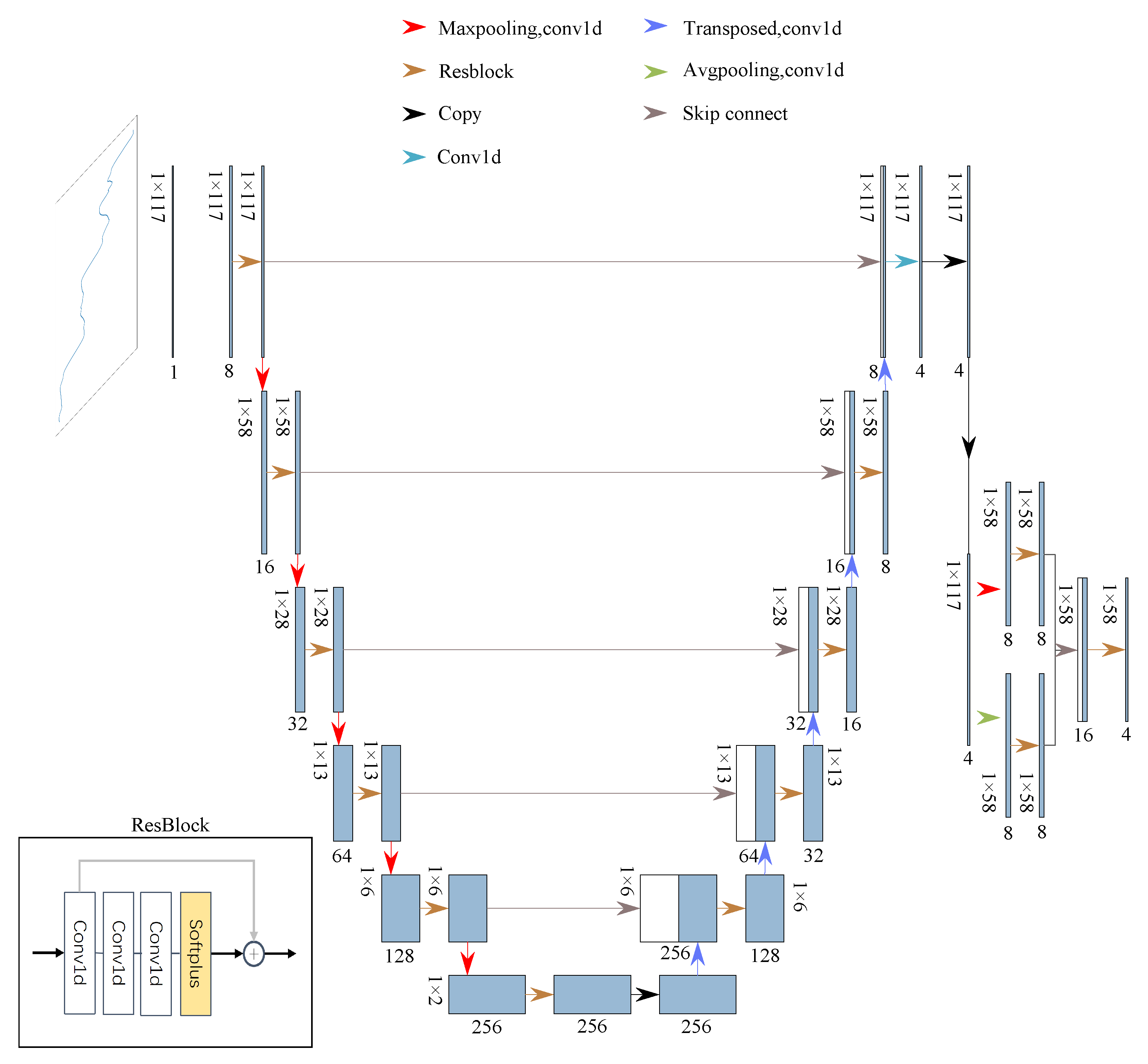
2.2. Revision of the U-Net

The original U-Net was introduced at the 2015 IEEE 12th International Symposium on Biomedical Imaging [14]. The U-Net is a variant of fully connected network architecture that retains the Encoder–Decoder structure. The Encoder part consists of convolution and downsampling operations that extract image feature information. A feature map is generated in each downsampling process. The Decoder part consists of deconvolution operations and performs upsampling on the feature maps. Unlike typical fully connected network structures, the U-Net uses skip-connections to fuse the feature maps from the downsampling process with the feature maps from the upsampling process. The authors claimed that this operation can compensate for the loss of edge features during downsampling. They achieved very good results without using huge data sets. Thus, we assumed a revised U-Net could provide a new tool for quantitative analysis.

Figure 1 shows our modified network structure. We modified all the 2D convolutional layers into 1D convolutional layers with a kernel size of 3 and a stride of 1. Thus, the revised U-Net can process 1D NIR spectra. At the same time, we constructed “ResBlocks” in our architecture. Each ResBlock is composed of three 1D convolutional layers and a residual network [20] followed by an activation operation called Softplus. The output from upsampling is introduced into a maximum pooling residual module (MPR) and an average pooling residual module (APR). The APR module consists of two residual convolutional layers to perform sampling through average pooling. The MPR module consists of two residual convolutional layers that extract features through maximum pooling.

These two modules extract feature information at different levels. The outputs from the APR and MPR modules are fused by channel concatenation. The fused layer is transferred into the final output. In Figure 1, the output channel is channel 4 and is aimed at CGL data. One can be changed into other values depending on their target property.

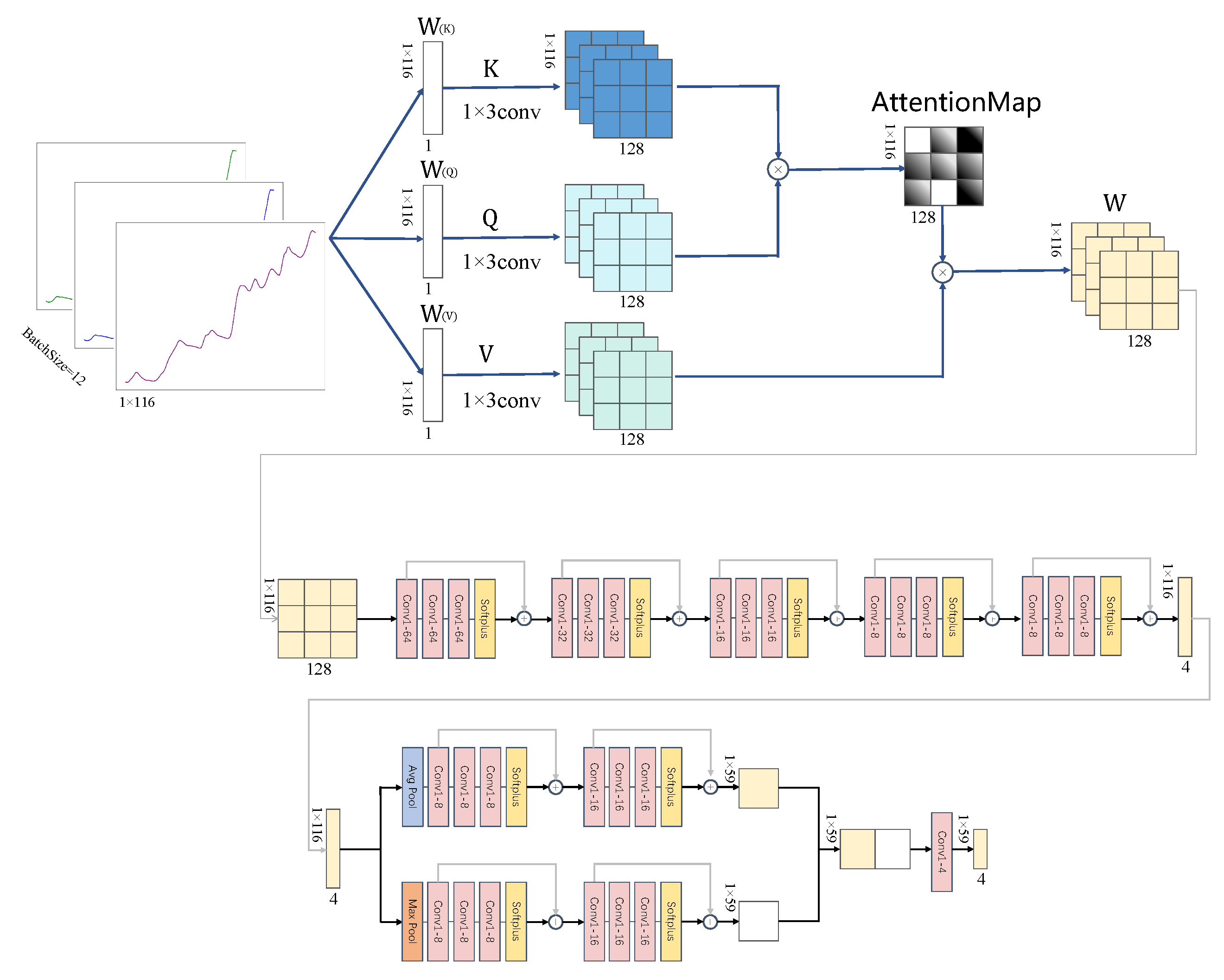
2.3. Revision of Attention Mechanism Network

The attention mechanism was one of the most influential discoveries in machine learning [15]. The attention mechanism performs well in capturing relatively small but important information from huge input data sets and thereby focuses on the important part. This capability makes the model more flexible and adaptable to various input data sets and tasks, and reduces the risk of redundant computation and overfitting. Compared to traditional DNNs, attention-mechanism-based DNNs can solve feature extraction and learning efficiency problems in a better way so as to achieve better performance. Although the attention mechanism was put forward for sequence-to-sequence models such as machine translation, we were attracted by its input pattern. The inputs of the attention mechanism are all vectorized information so this provides a chance to deal with quantitative-analysis-based NIR spectroscopy. In short, we expected that the attention mechanism will help capture important information in the NIR spectra for quantitative analysis.

Figure 2 shows our final constructed DNN architecture obtained by revising the attention mechanism. We made the following modifications to the network for the calculation of matrices $\mathbf{Q}$, $\mathbf{K}$ and $\mathbf{V}$, respectively: convolution with channel = 128, kernel size = 3, and step = 1. The selection of the number of channels, kernel size, and step size should be made according to the actual data situation. Adjustments need to be made for different data sets. The network diagram was adjusted for the CGL data set. We obtained it by multiplying the $\mathbf{Q}$ and $\mathbf{K}$ matrices and forming the attention distribution map through Softmax. The matrix obtained by Softmax was then multiplied with the following attention distribution weighted by the aggregate value vector of $\mathbf{V}$ to obtain a final output, which represents the fusion vector of the original set of input vectors. However, it is impossible to obtain a stable network by only relying on attention weight. In the second network, we also borrowed the idea of the ResNet [20]. We introduced the residual module to extract and continuously compress the data features. We gradually compressed the data from 128 channels to 4 channels to extract more details in the features. In our revised attention mechanism architecture, we also used the average pooling residual (APR) and maximum pooled residual (MPR) modules to compress the modules into 4 channels. Finally, we simultaneously averaged the spectral data by using the torch.mean(X, axis = 2) in relation to the corresponding components.

2.4. Hyperparameters and Evaluation Criteria

In this paper, the hyperparameters such as the filter number, the kernel size, the batch size, the learning rate ($LR$), etc., are similar to our previous work [13]. The setting of the hyperparameters is usually achieved by trial-and-error strategies [21]. Thus, we will not be concerned with the so-call optimized hyperparameters.

The $LR$ is still the following form:

$$LR=0.001\times 0.5^{\frac{iter}{10000}}$$

(1)

where $iter$ denotes the number of training iterations. The $LR$ was combined with an Adam optimizer in the training process.

The loss function is still the following form:

$$L=\frac{\left|\right|\mathbf{prediction}-\mathbf{property}\left|\right|}{\mathbf{property}}$$

(2)

where $\mathbf{property}$ denotes the quantities of substances and the $\mathbf{prediction}$ is the final output from the DNN.

The training process was conducted by minimizing the loss function, but the stop criterion was based on the determination coefficient $R^2$ between the $\mathbf{prediction}$ and $\mathbf{property}$. The minimum loss function value is theoretically the best value. In the practical training process, we cannot set the optimum threshold for the loss function. However, in quantitative analysis, $R^2\ge 0.95$ is a widely acceptable threshold. Our previous work [13] shows that using $R^2$ as stopping criterion was workable and satisfactory results were obtained. We also used root mean squared error (RMSE) as a reference evaluation criterion as follows:

$$RMSE=\sqrt{\frac{{\sum }_i^n{\left(propert{y}_i-predictio{n}_i\right)}^2}{n}}$$

(3)

All the codes for the neural networks were written in Python platform using PyTorch. The codes were run on a DELL Precision-3640-Tower workstation with an NVIDIA RTX 3090 graphics card of 24 GB of RAM. The operation system was the Ubuntu 20.04 LTS.

3. Results and Discussion

Our training strategy was aimed at achieving better accuracy of the resulting calibration model. Thus, we continuously increased the threshold of $R^2$ to obtain a better DNN architecture and hyperparameters. We aimed at obtaining acceptable network architecture but not the so-called optimized network architecture.

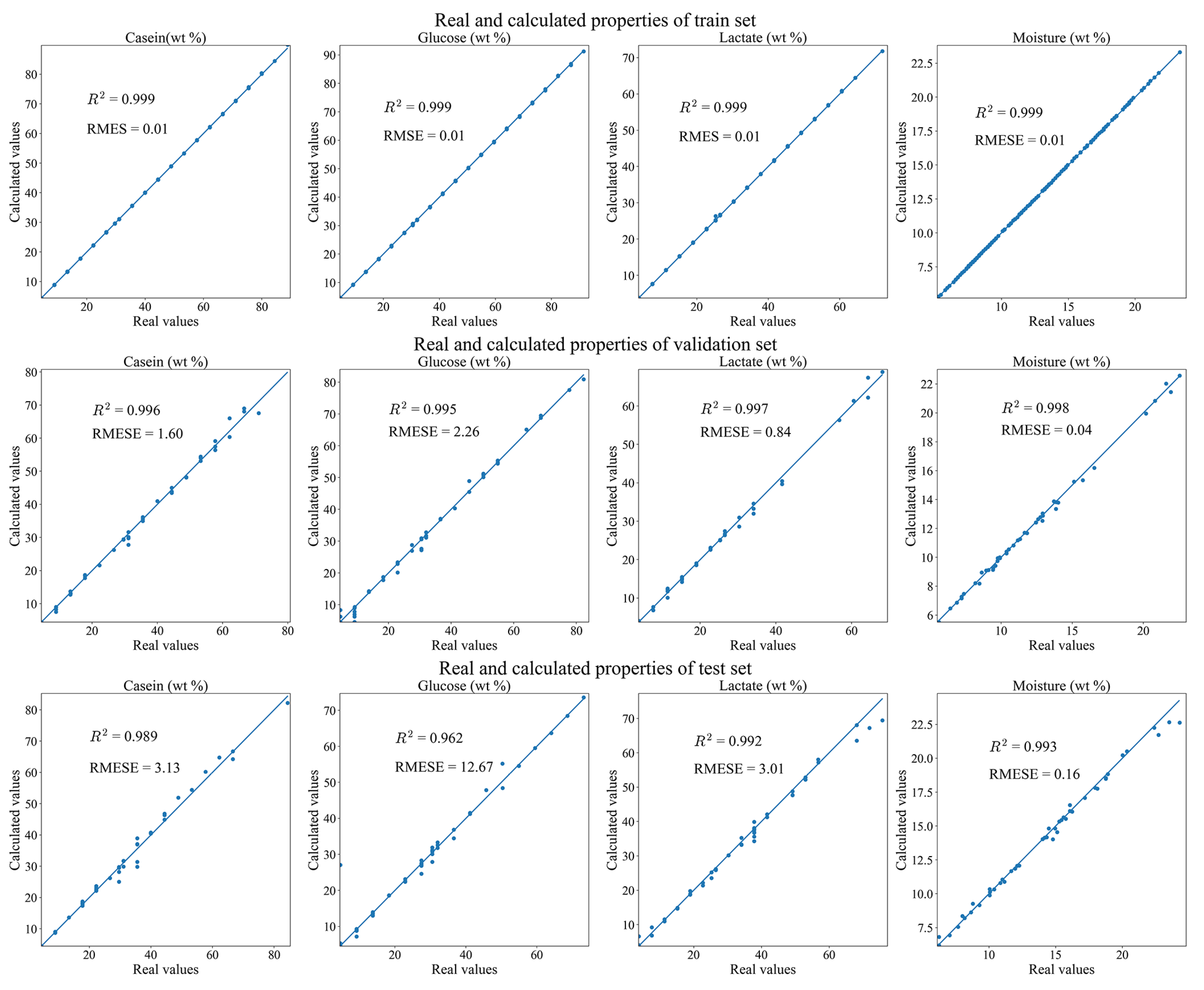
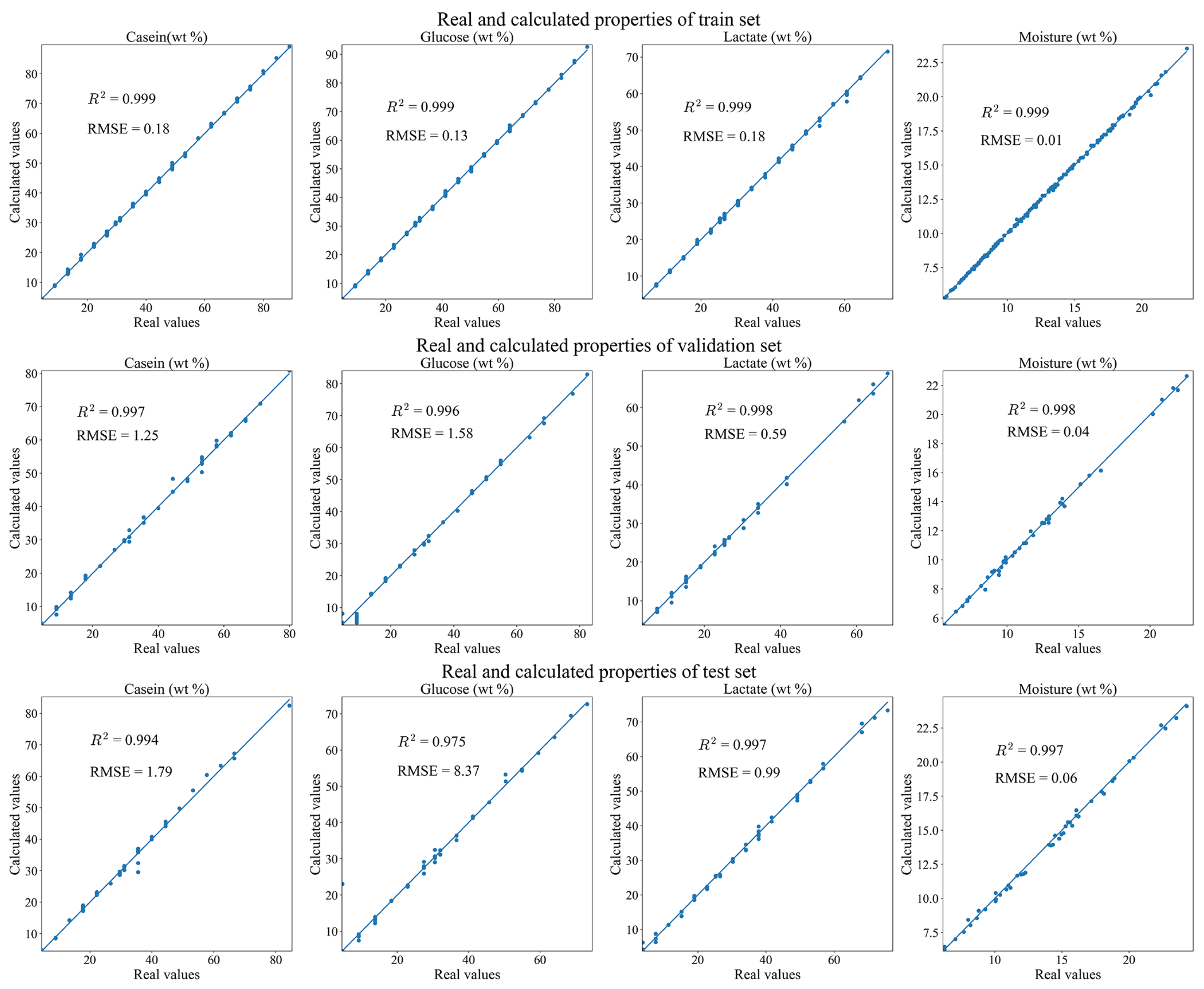
3.1. Two Revised DNNs Applied to the CGL Data Sets

Figure 3 shows the results of applying our revised U-Net DNN to the CGL data sets. The training set was used to train the model independently. The batch size is set at 12. The training process was focused on minimizing the loss function. In each of the training iterations, we obtained a temporary calibration model. We then conducted a random sampling to pick 12 samples from the training set and the validation set, respectively. We applied the temporary calibration model to the selected samples to obtain the calculated values of the four components and then to calculate the $R^2$ values from the reference values of the components. When the minimum values of $R^2$ for both the training set and the validation set reached the threshold of $R^2\ge 0.999$, we stopped the training process and obtained an acceptable calibration model.

The $R^2$ and $RMSE$ values shown in Figure 3 were calculated using the whole set of samples from the three data sets and not the 12 randomly picked samples. In this work, we continuously used this strategy in training our network and presenting our results. Compared with our previous work [13], the results shown in Figure 3 are adequate.

Figure 4 shows the results of applying our revised attention mechanism DNN to the CGL data sets. The results were still acceptable compared with the results shown in Figure 3 and our previous results [13]. The more important thing is that we still fulfill the goal of establishing a single calibration model for four species. So far, to our knowledge, no other researchers have reached that goal.

We did not try the transformer model architecture [15] because it is too complicated for us to find a reasonable way to use it. We did try multiple stacking of the attention module but failed to achieve better results in what was then a more complex model. Thus, we only used one attention module followed by the MPR and the APR modules. It might be that convolutional layers play the major role. However, these results mean that there may still room for further improvements.

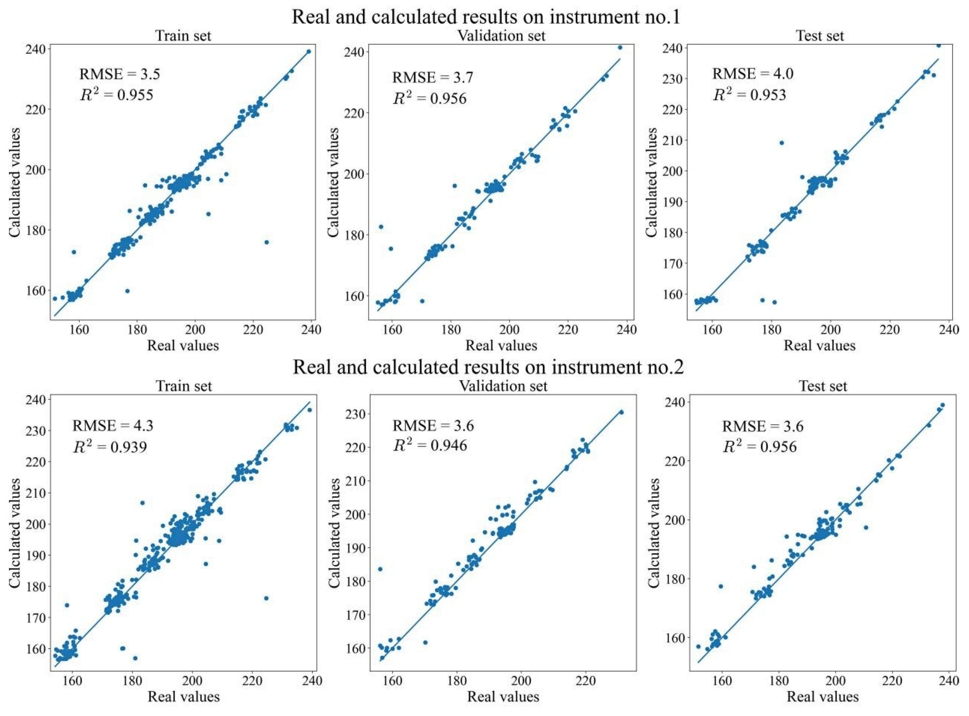
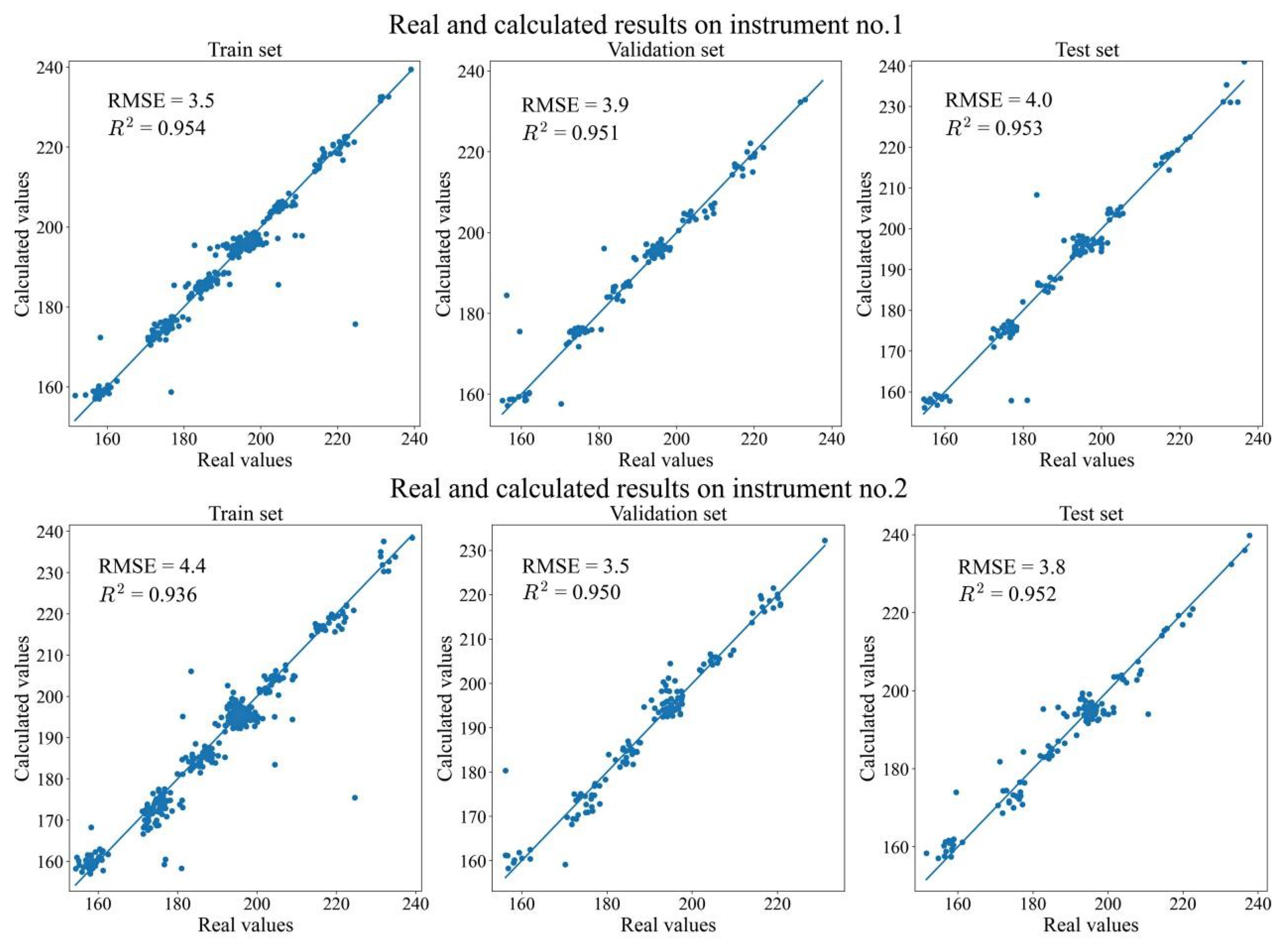
3.2. Two Revised DNNs Applied to the IDRC 2002 Data Sets

Figure 5 shows the revised U-Net DNN applied to the IDRC 2002 data sets. The threshold is set $R^2\ge 0.95$. The training process was based on IDRC 2002 set 1. The results are shown on the top subplots of Figure 5. One can see that the training, validation, and testing results are sufficient. The calibration model obtained from IDRC 2002 set 1 was then applied to IDRC 2002 set 2 and the results are shown in the bottom subplots of Figure 5. The results were also sufficient. Thus, the revised U-Net DNN can fulfill the goal of calibration transfer.

Figure 6 shows the application of the revised attention mechanism DNN applied to the IDRC 2002 data sets. The training process was applied to the IDRC-2002 set 1. The results are shown on the top subplots of Figure 6. The bottom subplots show the calibration transfer results using the obtained calibration model from IDRC 2002 set 1 applied to the IDRC-2002 set 2. The results were still acceptable and the calibration transfer was satisfactory.

One can see from Figure 5 and Figure 6 that some samples appear to be outliers. We did not make further efforts to determine the issues associated with them because it was outside the scope of the present work. The important thing is that we could use a small batch size of 12 in the training process and evaluate the threshold $R^2$. Furthermore, the obtained calibration model can be effectively applied to the whole data sets. Thus, this strategy can obtain a calibration model with good generalization capability.

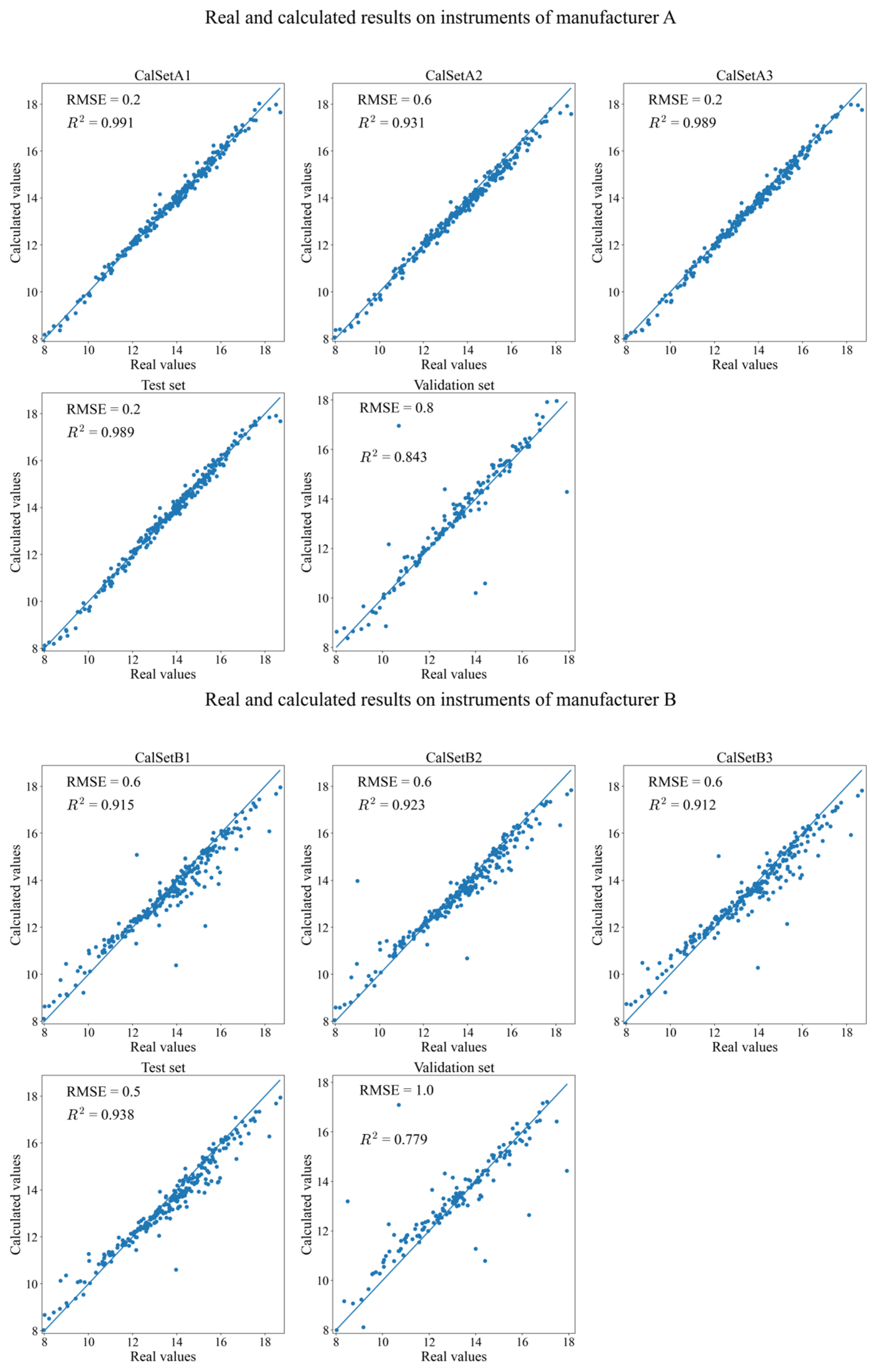
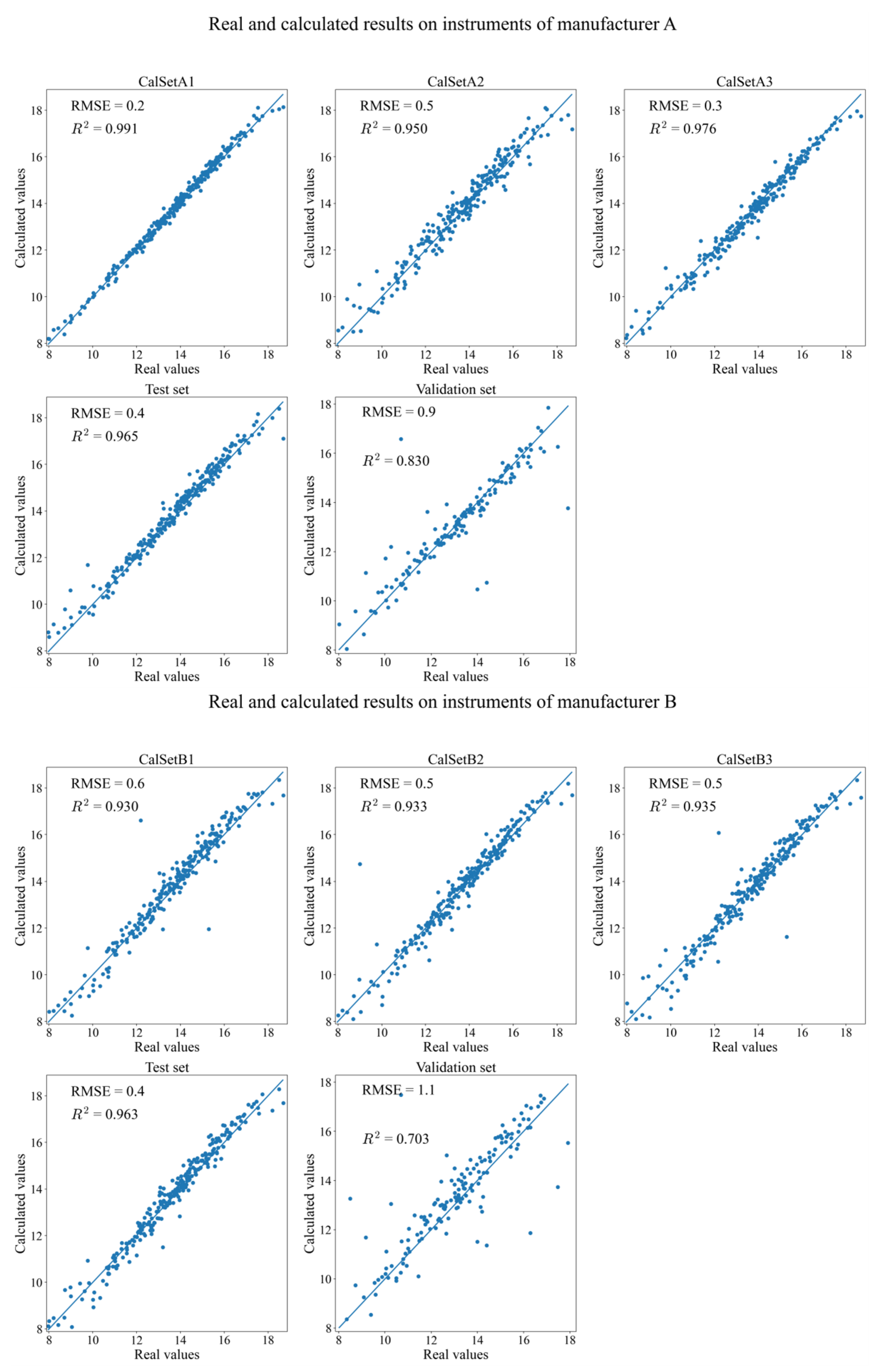
3.3. Two Revised DNNs Applied to the IDRC 2016 Data Sets

The IDRC 2016 ‘‘Shootout’’ data sets mainly aimed to provide a calibration transfer challenge. Calibration transfer means to establish a calibration model for one instrument and then apply it to other different instruments. This transfer is usually ineffective because the differences among the instruments will generate sufficiently different spectra even measuring same sample that the calibration fails. However, for a big enterprise that deploys many of the instruments at different locations, calibration transfer is a necessity that cannot be avoided. One can see from the IDRC 2016 report [19], some participants did obtain satisfactory results by combining multiple techniques. However, their success was highly dependent on the experience and skill of these skilled participants and may not be possible for typical users.

Figure 7 and Figure 8 show the results of applying the two revised DNNs to the data sets. We used the IDRC-2016 A1 in Table 1 as the training set (corresponding to CalSetA1 in Figure 7 and Figure 8) and the IDRC-2016 T (corresponding to Test set in Figure 7 and Figure 8) as the validation set in the training process. The threshold was set as $R^2\ge 0.99$. The obtained calibration model was then applied to calculate other data sets.

It can be seen that the results are sufficient when the calibration model was applied to the data sets from manufacturer A. However, somewhat poorer results were obtained when the calibration model was applied to the data sets from manufacturer B because the calibration model was established based on the measured data sets on the instrument of manufacturer A. Thus, for a large enterprise, deploying instruments from same manufacturer will be the best choice. Although the results were not fully satisfactory when the calibration model was applied to the unknown samples (Validation set in Figure 7 and Figure 8), these results are understandable because the unknown samples were developed to be the most challenging ones. It may be that there were intentionally designed spectra pretreatments, wavelength selections, calibration transfer techniques, etc. However, we did not apply pretreatment of the spectra. We did not use extra techniques such as the wavelength selection, and we did not use any other calibration transfer techniques. Thus, future work could be to develop DNN architectures that possess multiple abilities such as the most effective wavelength selection.

4. Conclusions

In this paper, two DNN architectures were successfully constructed; one was based on revising the U-Net and the other was based on revising the attention mechanism. The results showed that the two DNNs can be applied to quantitatively model NIR spectra. Thus, it is also potentially applicable to other types of spectroscopic data. The results of the CGL data showed that the DNN was a good tool for multiple-component quantitative analysis by providing convenience in its creation and the maintenance of the resulting calibration model. We see the DNNs provided the capability to cope with the challenging problem of calibration transfer even though the present results are not fully acceptable. Future work could be focused on how to capture the kernel information in the spectra related to the quantity of a component. We emphasize that replaying fully connected layer(s) with convolutional layers played an important role in our work. This approach could be a primary standard by which to judge the practicability of a DNNs in analytical chemistry.

References

1. Dong, A.; Zhang, L.; Liu, Z.; Liu, J.; Wei, Y. Advances in infrared spectroscopy and hyperspectral imaging combined with artificial intelligence for the detection of cereals quality. Crit. Rev. Food Sci. Nutr. 2022. [Google Scholar] [CrossRef]
2. Meza, C.P.; Santos, M.A.; Romañach, R.J. Quantitation of drug content in a low dosage formulation by transmission near infrared spectroscopy. AAPS Pharm. Sci. Tech. 2006, 7, 29. [Google Scholar] [CrossRef]
3. Shadrin, D.; Pukalchik, M.; Uryasheva, A.; Tsykunov, E.; Yashin, G.; Rodichenko, N.; Tsetserukou, D. Hyper-spectral NIR and MIR data and optimal wavebands for detection of apple tree diseases. arXiv 2020, arXiv:2004.02325. [Google Scholar]
4. Guo, Z.; Wang, M.; Agyekum, A.A.; Wu, J.; Chen, Q.; Zuo, M.; El-Seedi, H.R.; Tao, F.; Shi, J.; Ouyang, Q.; et al. Quantitative detection of apple watercore and soluble solids content by near infrared transmittance spectroscopy. J. Food Eng. 2020, 279, 109955. [Google Scholar] [CrossRef]
5. Pasquini, C. Near infrared spectroscopy: A mature analytical technique with new perspectives—A review. Anal. Chim. Acta 2018, 1026, 8–36. [Google Scholar] [CrossRef] [PubMed]
6. Chen, Y.Y.; Wang, Z.B. Quantitative analysis modeling of infrared spectroscopy based on ensemble convolutional neural networks. Chemom. Intell. Lab. Syst. 2018, 181, 1–10. [Google Scholar]
7. Xu, K.; Guo, J.; Song, B.; Cai, B.; Sun, H.; Zhang, Z. Interpretability for reliable, efficient, and self-cognitive DNNs: From theories to applications. Neurocomputing 2023, 545, 126267. [Google Scholar]
8. Zeng, J.; Guo, Y.; Han, Y.; Li, Z.; Yang, Z.; Chai, Q.; Wang, W.; Zhang, Y.; Fu, C. A Review of the Discriminant Analysis Methods for Food Quality Based on Near-Infrared Spectroscopy and Pattern Recognition. Molecules 2021, 26, 749. [Google Scholar] [CrossRef]
9. Qu, X.; Huang, Y.; Lu, H.; Qiu, T.; Guo, D.; Agback, T.; Orekhov, V.; Chen, Z. Accelerated nuclear magnetic resonance spectroscopy with deep learning. Angew. Chem. Int. Ed. 2020, 59, 10297–10300. [Google Scholar] [CrossRef] [Green Version]
10. Gabrieli, G.; Bizzego, A.; Neoh, M.J.Y.; Esposito, G. fNIRS-QC: Crowd-Sourced Creation of a Dataset and Machine Learning Model for fNIRS Quality Control. Appl. Sci. 2021, 11, 9531. [Google Scholar] [CrossRef]
11. Rankine, C.D.; Madkhali, M.M.M.; Penfold, T.J. A deep neural network for the rapid prediction of X-ray absorption spectra. J. Phys. Chem. 2020, 124, 4263–4270. [Google Scholar] [CrossRef] [PubMed]
12. Le, B.T. Application of deep learning and near infrared spectroscopy in cereal analysis. Vib. Spectrosc. 2020, 106, 103009. [Google Scholar] [CrossRef]
13. Gan, F.; Luo, J. Simple dilated convolutional neural network for quantitative modeling based on near infrared spectroscopy techniques. Chemom. Intell. Lab. Syst. 2023, 232, 104710. [Google Scholar] [CrossRef]
14. Ronneberger, O.; Fischer, P.; Brox, T. U-Net: Convolutional Networks for Biomedical Image Segmentation. arXiv 2015, arXiv:1505.04597. [Google Scholar]
15. Vaswani, A.; Shazeer, N.; Parmar, N.; Uszkoreit, J.; Jones, L.; Gomez, A.N.; Kaiser, L.; Polosukhin, I. Attention is All you Need. arXiv 2017, arXiv:1706.03762. [Google Scholar]
16. Guo, S.; Mayerhöfer, T.; Pahlow, S.; Hübner, U.; Popp, J.; Bocklitz, T. Deep learning for ’artefact’ removal in infrared spectroscopy. Analyst 2020, 145, 5213–5220. [Google Scholar] [CrossRef] [PubMed]
17. Wang, Z.; Zhang, J.; Zhang, X.; Chen, P.; Wang, B. Transformer Model for Functional Near-Infrared Spectroscopy Classification. IEEE J. Biomed. Health Infor. 2022, 26, 2559–2569. [Google Scholar] [CrossRef]
18. McClure, F. IDRC-2002. NIR News. 2002, 13, 3–5. [Google Scholar] [CrossRef]
19. Igne, B.; Alam, M.A.; Bu, D.; Dardenne, P.; Feng, H.; Gahkani, A.; Hopkins, D.W.; Mohan, S.; Hurburgh, C.R.; Brenner, C. Summary of the 2016 IDRC software shoot-out. NIR News 2017, 28, 16–22. [Google Scholar] [CrossRef]
20. He, K.M.; Zhang, X.Y.; Ren, S.Q.; Sun, J. Deep Residual Learning for Image Recognition. arXiv 2015, arXiv:1512.03385. [Google Scholar]
21. Debus, B.; Parastar, H.; Harrington, P.; Kirsanov, D. Deep learning in analytical chemistry. TrAC-Trend Anal. Chem. 2021, 145, 116459. [Google Scholar] [CrossRef]
Figure 1. Our DNN architecture by revising U-Net architecture (Model 1).
Applsci 13 08494 g001
Figure 2. Our DNN architecture created by revising the attention mechanism (Model 2). Although we had tried stacking multiple attention modules, finally we only used one because no significant improvements were obtained based on the multiple module approach. Multiple 1D convolutional layers are still the major part of our revisions.
Applsci 13 08494 g002
Figure 3. Predicted versus measured plots of the training set, validation set and test set using revised U-Net DNN.
Applsci 13 08494 g003
Figure 4. Predicted versus measured plots of the training set, validation set and test set using revised attention mechanism DNN.
Applsci 13 08494 g004
Figure 5. Predicted versus measured quantities of the active substance of the Escitalopramt tablets based on the revised U-Net DNN.
Applsci 13 08494 g005
Figure 6. Predicted versus measured quantities of the active substance of the Escitalopramt tablets based on the revised attention mechanism DNN.
Applsci 13 08494 g006
Figure 7. Predicted versus measured plots of the all data sets based on an acceptable quantitative model established from the NIR spectra of CalSetA1 of manufacturer A using the revised U-Net DNN.
Applsci 13 08494 g007
Figure 8. Predicted versus measured plots of the all data sets based on an acceptable quantitative model established from the NIR spectra of CalSetA1 of manufacturer A using the revised attention mechanism DNN.
Applsci 13 08494 g008