Metrics Related to Confusion Matrix as Tools for Conformity Assessment Decisions

Featured Application

Application in determining optimal length of the guard band when assessing global producer’s and consumer’s risk.

Abstract

Conformity assessment refers to activities undertaken to check whether some product, service or process meets certain criteria and specifications given by internationally accepted standards. The decision on whether a property of interest is aligned with the set standards is made based on measurement. However, uncertainty associated with the measurement results may lead to incorrect decisions. Measurement results may be falsely rejected as non-conforming, although they meet specifications. This is referred to as the producer’s risk. If the measurement result that does not meet the required specifications is accepted as conforming, this is referred to as the consumer’s risk. This paper covers calculations of global consumer's and producer's risk using the Bayesian approach and deals with the application of metrics related to confusion matrices in conformity assessments. These techniques have been used to assess the conformity of the bearing ring diameter with the given specifications. Based on the behavior of these metrics, the optimal length of the guard band was determined with the aim of minimizing the global consumer’s and producer’s risk.

1. Introduction

The guidelines for conformity assessment of an item of interest were adopted by the Joint Committee for Guides in Metrology (JCGM) and are given by guide 106:2012 [1]. The item of interest must meet certain specifications prescribed by the norms or given externally by the manufacturer. The fulfilment of these requirements mainly refers to the fact that the value of the tested characteristic of the specific tested item must be within the set limits of the tolerance interval. The decision on the compliance of an item of interest with the given standards can be made by using a simple binary decision rule. The item of interest is conformed with the specifications if the measured value of the characteristic under test lies within the tolerance interval. Otherwise, the item of interest does not comply with the specifications. When applying a simple binary rule, apart from these two outcomes, there are no other outcomes that would indicate the state where no decision can be made for the property of interest.

For a typical product obtained in a production process, the probability of rejecting a conforming product is called a specific producer’s risk. The probability of accepting a non-compliant product is called specific consumer risk. If the nominal value of the measurand and measurement uncertainty for the performed measurements are known, both probabilities can be calculated using conformance probability $p_C$ [2].

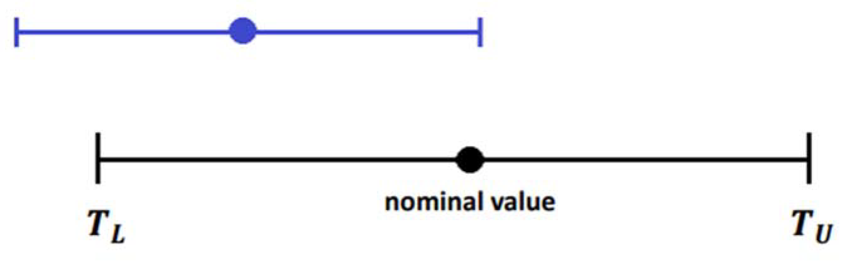
The measurement result is complete if it comprises the measured value and the associated measurement uncertainty. Measurement uncertainty represents the quality of the measurement result. Only the result with measurement uncertainty can be used for comparing results with specifications. However, uncertainty associated with the measurement results may lead to incorrect decisions. Relying on a simple binary decision rule and measured values from a normal distribution can result in a probability of accepting a nonconforming item or rejecting a conforming item as low as 50% [3,4,5,6]. This happens when the measurement uncertainty of the measured item is high, and the measured value is near the upper or lower limit of the tolerance interval (Figure 1).

To reduce this type of risk, an acceptance interval is introduced in the conformity assessment procedure [7,8,9]. The tolerance and acceptance interval can be in different relations [10]. In the case of a simple binary decision rule, the limits of the tolerance interval and the acceptance interval coincide (Figure 2b). That decision rule is also called shared risk. To decrease the producer’s risk, the acceptance interval has been set to comprise the tolerance interval (Figure 2a). If the tolerance interval comprises the acceptance interval, the intention is to minimize the consumer’s risk (Figure 2c).

By introducing acceptance intervals, the concept of conformity assessment is extended to more general decision problems. In this case, four different outcomes are possible. Valid acceptance occurs when the measured value is within the acceptance interval and satisfies the specifications. Valid rejection occurs when the measured value is outside the tolerance interval and outside the acceptance interval. In terms of machine learning, valid acceptance is equivalent to the term true positive (TP), and the term valid rejection is equivalent to the term true negative (TN). If an item is accepted but does not conform to specifications, this is called false acceptance (FA). False acceptance probability refers to the global consumer’s risk. If the measurement result is rejected, although it conforms to a specification, this is a falsely rejected measurement (FR). The probability of this incorrect decision is called the global producer’s risk. In contrast to the specific risk related to a particular tested item, the global risk of producers and consumers refers to the risks calculated for a sample drawn from some statistical population of such items obtained in some production process [1].

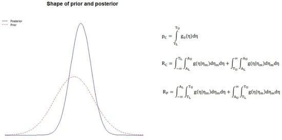
Foremost, the calculation of risk, specific and global, is carried out due to the improvement of the production process, the reduction of scrap, i.e., the number of products that do not meet the given standards, and the reduction of the producer’s costs. Also, consumer risk assessment provides the probability of purchasing a defective product. The global consumers’ and producers’ risks are calculated using the Bayesian approach [11,12]. The Bayesian approach combines two sources of information. The first source of information refers to prior beliefs of a measurer about the possible distribution of parameters that describes the measurement data. In addition, such a source of information can be the results of previous measurements, data from manuals, historical data, etc. [13]. These data are treated as a random variable Y, and they are expressed by the probability density function (PDF), which is usually called a prior, denoted by $g_0\left(\eta \right)$. The values that take by the prior are marked with $\eta$. According to the principle of maximum entropy (PME), when the first two moments of the distribution are known, in this case, that is the best estimate of a measurand $\overline{y}$, and the standard measurement uncertainty $u_0$, the prior is usually a two-parameter distribution [14]. Considering that these data are an outcome of a measurement, the prior is usually a normal distribution. Depending on the nature of the measurand and the number of known moments, other two-parameter distributions can be used, as well as one-parameter or non-parametric distributions [9,15].

The second source of information is data assigned to the measurements. These data are also regarded as a random variable $Y_m$, and they are expressed via the likelihood function for normal distribution denoted by $h\left({\eta }_m|\eta \right)$. Likelihood function formula includes standard measurement uncertainty $u_m.$ Values of the likelihood function are denoted by ${\eta }_m$. It is important to notice that according to Bayes’ rule, the prior distribution is independent of the likelihood function, so data for one and the other function must come from different sources. Thus, data for the likelihood function are usually obtained from subsequent production process quality control [1] (pp. 27–32).

Determining the global risk of producers and consumers according to the Bayesian approach requires the numerical solution of the double integral. This procedure involves knowledge of programming that can be difficult for users to apply, especially if Monte Carlo methods are required for the posterior distribution simulation [6,16,17]. Therefore, risk calculation is often avoided in the quality control of the production process. However, such an attitude is wrong. Since the risks of the consumer and producer are related, the producer can reduce his costs by assessing the risk and, at the same time, guaranteeing the consumer a certain level of product quality.

The conformity assessment procedure can be applied in a wide range of disciplines. For example: in the assessment of the efficiency of liquid chromatography analytical procedures [18], as a tool in the pharmaceutical industry for drug quality control [19], for the evaluation of the risk of a false decision on compliance of multicomponent materials [20], for quality evaluation of automotive fuels [21], or in a food control [22]. Examples above represent multivariant models, where total risk is being assessed. When assessing the total risk, each of the tested components must meet the specifications that apply to it and that are related to the characteristic property that is tested for that individual component. Conformity assessment procedure can also be used in a simple univariate case when only one characteristic is assessed, as in the assessment process of the epoxy coating thickness applied on water pipes [23], or in water quality control [24].

In this paper, the global risk of producers and consumers was assessed. The risk is calculated to evaluate the conformity of the inner diameter of the ring with the required specifications. The formulas for determining these risks are in themselves a kind of classifier that classifies the measurement results into categories TP, TN, FA, and FR [25]. These categories form a square confusion matrix 2 × 2, a well-known concept from machine learning. Contrary to machine learning, where the classification is performed on a large amount of data split into training and test sets, here, the classification is performed based on the relationship between the conformance probability and the global producer’s and consumer’s risk. For this type of classification, it is sufficient to have the data obtained by measurement and the associated measurement uncertainty. To evaluate the performance of the tested models, the metrics associated with the confusion matrices were used. Of the many metrics used, the most common are accuracy, precision, recall, and F1 score [26,27]. In this paper, other metrics, apart from these basic metrics, were observed, especially those assumed to be well-behaved on imbalanced data that primarily occur in metrology, such as Cohen’s kappa statistic and Mathew’s correlation coefficient (MCC) [28,29]. Using these metrics, the optimal length of the guard band between the tolerance interval and the acceptance interval was determined in terms of minimizing the global risk of consumers and producers.

2. Materials and Methods

2.1. Production Process and Improvement Procedure

In this paper, the effect of measurement uncertainty on conformity assessment has been analyzed based on the measurement of the inner diameter of a bearing ring. By monitoring the production process and quality control process in one Croatian company, it was established that there is a significant percentage of non-conforming units. The existing quality control was conducted by workers after each production phase using manual gauges and devices for controlling measurements (Figure 3).

Specific dimensions and geometric characteristics of the bearing ring were 100% controlled, while the others were sampled for control by randomly choosing 3 to 10 products. Such a control system did not always ensure the delivery of conforming products. Because of this, the existing product quality control process had to be changed. Changes have involved the implementation of the new automated measurement system (Figure 4). The new measurement system enabled the conducting of measurements of specified dimensions and geometric characteristics in 100% of cases, as well as monitoring production process capabilities and measurement system quality. In addition, the new automated system can continuously monitor and store results and sort products (separating bad products from good products). Although the purpose of quality control is not sorting products, but rather obtaining and maintaining control over the process and continuous improvement of the process; the goal of sorting the products is to minimize the possibility of customers receiving a non-conforming product. An automated measurement system removes the human factor from the measurement process, which significantly reduces the measurement uncertainty of measurement results. Continuous monitoring and analysing measurement results enables for timely response during the production process and, thus, prevents the manufacturing of non-conforming products. When the measurement system detects a non-conforming product, that particular product will not be delivered to the customer. However, regardless of the quality of a measurement system, the measurement system will always comprise measurement uncertainty, which can lead to making wrong decisions. To this end, this paper analyses the effect of measurement uncertainty on global producer’s and consumer’s risk, which is why the optimal acceptance interval limit has to be determined. This paper analyses risk based on the measurement of the inner diameter of a bearing ring, with a nominal value of 100 mm. According to the producer’s specifications, tolerance field for inner diameter equals ± 0.022 mm. The effect of measurement uncertainty on non-conformity assessment was observed for the inner diameter of the bearing ring because that dimension was 100% controlled using the initial (previous) and improved (new) measurement system. Following experimental results of two measurement systems (initial and improved) were used as input data for the mathematical model. The nominal value of the inner diameter of the ring of the initial model is $\overline{y}=100.008$ mm with standard deviation of $u_0=0.011$ mm. The subsequent inspection process was carried out with a measurement uncertainty of $u_m=0.005$ mm. With the improved production process for the nominal value of the inner diameter of the ring, it was obtained by measurement that $\overline{y}=100.004$ mm with standard deviation of $u_0=0.0066$ mm. The measurement uncertainty of the control quality process associated with the improved model amounts to $u_m=0.0015$ mm. In the further text, the terms improved model, improved process, and improved measurement system are identified. The same applies for the term initial model.

2.2. Risk Calculation

According to [1], the probability that the measured value of the inner diameter of the ring is within the tolerance field is given by the expression for conformance probability:

$${\mathrm{p}}_{\mathrm{C}}=\underset{{\mathrm{T}}_{\mathrm{L}}}{\overset{{\mathrm{T}}_{\mathrm{U}}}{{\displaystyle \int }}}{\mathrm{g}}_0\left(\mathsf{\eta }\right)\mathrm{d}\mathsf{\eta }.$$

(1)

The lower and upper limits of the tolerance interval are marked with $T_L$ and $T_U,$ respectively. The sub integral function, i.e., prior, in expression (1), for conformance probability, is the normal distribution $Y~N\left(\overline{y},u_0\right)$ and, according to the [1]:

$${\mathrm{g}}_0\left(\mathsf{\eta }\right)=\frac{1}{{\mathrm{u}}_0\sqrt{2\mathsf{\pi }}}\exp \left[-\frac{1}{2}{\left(\frac{\mathsf{\eta }-\overline{\mathrm{y}}}{{\mathrm{u}}_0}\right)}^2\right].$$

(2)

In contrast to the centered examples in a norm JCGM 106:2012, the initial and the improved process over here are non-centered, which means that the nominal value $\overline{y}$ is not in the middle of the tolerance interval [1] (pp. 27–32).

Data obtained by subsequent control sampling were modelled using the likelihood function for a normal distribution, according to the [1] following is worth:

$$\mathrm{h}\left({\mathsf{\eta }}_{\mathrm{m}}|\mathsf{\eta }\right)=\frac{1}{{\mathrm{u}}_{\mathrm{m}}\sqrt{2\mathsf{\pi }}}\exp \left[-\frac{1}{2}{\left(\frac{{\mathsf{\eta }}_{\mathrm{m}}-\mathsf{\eta }}{{\mathrm{u}}_{\mathrm{m}}}\right)}^2\right].$$

(3)

To determine the global producer’s and consumer’s risk, it is necessary to set the lower and upper limits of the acceptance interval. The initial value of the total length of the guard band ${\mathrm{w}}_{\mathrm{U}}$, for both models, initial and improved, was set to ${\mathrm{w}}_{\mathrm{U}}=0.005$ mm. The maximum length of the guard band on each side is equal $\mathrm{w}=0.0025$ mm. In general, the length of the guard band depends on the multiplicative factor $\mathrm{r}\in \left[-1,1\right]$, and it can be calculated as follows:

$$\mathrm{w}=\frac{\mathrm{r}·{\mathrm{w}}_{\mathrm{U}}}{2}.$$

(4)

Now the lower limit of the acceptance interval $A_L$ is calculated as follows:

$${\mathrm{A}}_{\mathrm{L}}={\mathrm{T}}_{\mathrm{L}}+\frac{\mathrm{r}·{\mathrm{w}}_{\mathrm{U}}}{2},$$

(5)

and the upper limit of the acceptance $A_U$ from:

$${\mathrm{A}}_{\mathrm{U}}={\mathrm{T}}_{\mathrm{U}}-\frac{\mathrm{r}·{\mathrm{w}}_{\mathrm{U}}}{2}.$$

(6)

For $\mathrm{r}ϵ[-1,0\rangle$, the tolerance interval is within the acceptance interval (Figure 2a). This is the case of the minimization of the global producer’s risk. For $\mathrm{r}=0$, it holds that $\left[{\mathrm{A}}_{\mathrm{L}},{\mathrm{A}}_{\mathrm{U}}\right]=\left[{\mathrm{T}}_{\mathrm{L}},{\mathrm{T}}_{\mathrm{U}}\right]$ (Figure 2b). The acceptance interval is within the tolerance interval for $\mathrm{r}ϵ\langle 0,1]$ (Figure 2c). This is a model of minimization of the global consumer’s risk.

The next step is the subdivision of the interval $\left[-1,1\right]$, which is the domain of the multiplicative factor $r$. The subdivision rate is equidistant and equal to $0.1$. The subdivision resulted in 21 nodes. For different values of the multiplying factor $r$, according to Formula (4), different lengths of the guard band $\mathrm{w}$ were obtained. For each of the nodes, from Formulas (5) and (6) are determined the lower and upper limits of the acceptance interval.In this way, all the necessary components for determining the global producer's and consumer's risk were defined.

According to Bayes’ theorem, a posterior distribution has the following formula, [1]:

$$\mathrm{g}\left(\mathsf{\eta }|{\mathsf{\eta }}_{\mathrm{m}}\right)=\mathrm{C}·{\mathrm{g}}_0\left(\mathsf{\eta }\right)\mathrm{h}\left({\mathsf{\eta }}_{\mathrm{m}}|\mathsf{\eta }\right).$$

(7)

The constant $\mathrm{C}$ is a normalization constant chosen so that holds ${{\displaystyle \int }}_{-\infty }^{\infty }g\left(\eta |{\eta }_m\right)d\eta =1$.

If the measured value $Y_m$ is within the acceptance interval, and if the true value Y of the item of interest is outside the tolerance interval, according to [1], the global consumer’s risk can be calculated as follows:

$${\mathrm{R}}_{\mathrm{C}}={{\displaystyle \int }}_{-\infty }^{{\mathrm{T}}_{\mathrm{L}}}{{\displaystyle \int }}_{{\mathrm{A}}_{\mathrm{L}}}^{{\mathrm{A}}_{\mathrm{U}}}\mathrm{g}\left(\mathsf{\eta }|{\mathsf{\eta }}_{\mathrm{m}}\right){\mathrm{d}\mathsf{\eta }}_{\mathrm{m}}\mathrm{d}\mathsf{\eta }+{{\displaystyle \int }}_{{\mathrm{T}}_{\mathrm{U}}}^{\infty }{{\displaystyle \int }}_{{\mathrm{A}}_{\mathrm{L}}}^{{\mathrm{A}}_{\mathrm{U}}}\mathrm{g}\left(\mathsf{\eta }|{\mathsf{\eta }}_{\mathrm{m}}\right){\mathrm{d}\mathsf{\eta }}_{\mathrm{m}}\mathrm{d}\mathsf{\eta }.$$

(8)

If the measured value $Y_m$ is outside the acceptance interval, and if the true value Y of item of the interest is within the tolerance interval, global producer’s risk, according to [1], is given by:

$${\mathrm{R}}_{\mathrm{P}}={{\displaystyle \int }}_{-\infty }^{{\mathrm{A}}_{\mathrm{L}}}{{\displaystyle \int }}_{{\mathrm{T}}_{\mathrm{L}}}^{{\mathrm{T}}_{\mathrm{U}}}\mathrm{g}\left(\mathsf{\eta }|{\mathsf{\eta }}_{\mathrm{m}}\right){\mathrm{d}\mathsf{\eta }}_{\mathrm{m}}\mathrm{d}\mathsf{\eta }+{{\displaystyle \int }}_{{\mathrm{A}}_{\mathrm{U}}}^{\infty }{{\displaystyle \int }}_{{\mathrm{T}}_{\mathrm{L}}}^{{\mathrm{T}}_{\mathrm{U}}}\mathrm{g}\left(\mathsf{\eta }|{\mathsf{\eta }}_{\mathrm{m}}\right){\mathrm{d}\mathsf{\eta }}_{\mathrm{m}}\mathrm{d}\mathsf{\eta }.$$

(9)

Considering that the cumulative distribution function (CDF) for the unit normal distribution is given by:

$$\mathsf{\varphi }\left(\mathrm{z}\right)=\frac{1}{\sqrt{2\mathsf{\pi }}}{{\displaystyle \int }}_{-\infty }^{\mathrm{z}}\exp \left(-\frac{{\mathrm{t}}^2}{2}\right)\mathrm{dt}={{\displaystyle \int }}_{-\infty }^{\mathrm{z}}{\mathsf{\phi }}_0\left(\mathrm{t}\right)\mathrm{dt},$$

(10)

where ${\phi }_0$ is the density function of the standard normal distribution. By introducing substitutions:

$$\mathrm{v}=\frac{{\mathsf{\eta }}_m-\mathsf{\eta }}{{\mathrm{u}}_m}.$$

(11)

$$\mathrm{z}=\frac{\mathsf{\eta }-\overline{\mathrm{y}}}{{\mathrm{u}}_0}.$$

(12)

it can easily be calculated that:

$$\frac{1}{{\mathrm{u}}_{\mathrm{m}}\sqrt{2\mathsf{\pi }}}{{\displaystyle \int }}_{{\mathrm{A}}_{\mathrm{L}}}^{{\mathrm{A}}_{\mathrm{U}}}\exp \left[-\frac{1}{2}{\left(\frac{{\mathsf{\eta }}_{\mathrm{m}}-\mathsf{\eta }}{{\mathrm{u}}_{\mathrm{m}}}\right)}^2\right]{\mathrm{d}\mathsf{\eta }}_{\mathrm{m}}=\mathsf{\varphi }\left(\frac{{\mathrm{A}}_{\mathrm{U}}-\overline{\mathrm{y}}-{\mathrm{zu}}_0}{{\mathrm{u}}_{\mathrm{m}}}\right)-\mathsf{\varphi }\left(\frac{{\mathrm{A}}_{\mathrm{L}}-\overline{\mathrm{y}}-{\mathrm{zu}}_0}{{\mathrm{u}}_{\mathrm{m}}}\right).$$

(13)

By introducing label

$$\mathrm{F}\left(\mathrm{z}\right)=\mathsf{\varphi }\left(\frac{{\mathrm{A}}_{\mathrm{U}}-\overline{\mathrm{y}}-{\mathrm{zu}}_0}{{\mathrm{u}}_{\mathrm{m}}}\right)-\mathsf{\varphi }\left(\frac{{\mathrm{A}}_{\mathrm{L}}-\overline{\mathrm{y}}-{\mathrm{zu}}_0}{{\mathrm{u}}_{\mathrm{m}}}\right),$$

(14)

as it was shown in [1], and considering Equations (2), (5) and (6), specified substitutions (11) and (12), the general expressions (8), global consumer’s risk takes the following form:

$${\mathrm{R}}_{\mathrm{C}}=\underset{-\infty }{\overset{\frac{{\mathrm{T}}_{\mathrm{L}}-\overline{\mathrm{y}}}{{\mathrm{u}}_0}}{{\displaystyle \int }}}{\mathsf{\phi }}_0\left(\mathrm{z}\right)\mathrm{F}\left(\mathrm{z}\right)\mathrm{dz}+\underset{\frac{{\mathrm{T}}_{\mathrm{U}}-\overline{\mathrm{y}}}{{\mathrm{u}}_0}}{\overset{\infty }{{\displaystyle \int }}}{\mathsf{\phi }}_0\left(\mathrm{z}\right)\mathrm{F}\left(\mathrm{z}\right)\mathrm{dz}.$$

(15)

The expression for the global producer’s risk, according to [1], assumes the form:

$${\mathrm{R}}_{\mathrm{P}}=\underset{\frac{{\mathrm{T}}_{\mathrm{L}}-\overline{\mathrm{y}}}{{\mathrm{u}}_0}}{\overset{\frac{{\mathrm{T}}_{\mathrm{U}}-\overline{\mathrm{y}}}{{\mathrm{u}}_0}}{{\displaystyle \int }}}{\mathsf{\phi }}_0\left(\mathrm{z}\right)\left(1-\mathrm{F}\left(\mathrm{z}\right)\right)\mathrm{dz}.$$

(16)

Global consumer’s risk represents the probability that the product has been falsely accepted as conforming to specifications. Global producer’s risk represents probability that the product has been falsely rejected as non-conforming while conforming to specifications.

Expressions (15) and (16) for global consumer’s and producer’s risks have been somewhat simplified with regards to general Formulas (8) and (9), but numerical integration is still required. The procedure for deriving Formulas (15) and (16) is superficially described in [1]. A more detailed derive is demonstrated here.

2.3. Confusion Matrix Construction

Equations (15) and (16) for global consumer’s and producer’s risk, respectively, represent a classifier similar to the naive Bayes classifier utilized in machine learning. Both are based on applying Bayes’ theorem and combining prior distribution and likelihood functions [30]. From the definition of these risks, it follows that they classify data into FA and FR categories, and the following is worth:

$$\mathrm{FA}={\mathrm{R}}_{\mathrm{C}},$$

(17)

$$\mathrm{FR}={\mathrm{R}}_{\mathrm{P}}.$$

(18)

According to norm JCGM 106:2012, there is a direct relationship between conformance probability, the global producer’s risk, and the number of rings that conformed to specifications, [1]. This connection is given by:

$$\mathrm{TP}={\mathrm{p}}_{\mathrm{C}}-{\mathrm{R}}_{\mathrm{P}}.$$

(19)

Analogously, the number of validly rejected rings is given as:

$$\mathrm{TN}=1-{\mathrm{p}}_{\mathrm{C}}-{\mathrm{R}}_{\mathrm{C}}.$$

(20)

In this way, without a training set and without a test set, all elements of the confusion matrix were determined. Each of the 21 values of the multiplier $r$ has been associated with one confusion matrix. For each confusion matrix, the values of the associated metrics were calculated. Thus, the behavior of the metrics can be monitored on the entire tolerance interval or the entire acceptance interval, depending on the mutual positions of these intervals. In meteorological terms, the confusion matrix now looks like in Figure 5.

2.4. Metrics Associated to Confusion Matrix Written in Metrology Manner

Unlike the standard expressions for metrics associated with confusion matrices used in machine learning [31], all observed metrics here have been written using expressions specified in Formulas (17)–(20). Accuracy is included in basic metrics that are used to evaluate the behavior of tested models. Originally, this metric details the ratio between the number of rings classified into the TP and TN categories in relation to the total number of rings. In risk assessment, always applies $TP+TN+FA+FR=1.$ That is why the accuracy metric in the conformity assessment procedure actually measures the total number of rings classified in the TP and TN categories and can be calculated as:

$$\mathrm{accuracy}=1-{\mathrm{R}}_{\mathrm{P}}-{\mathrm{R}}_{\mathrm{C}}.$$

(21)

The precision metric gives the ratio of rings classified as TP in relation to the total number of rings within the acceptance interval. In risk terms, the precision can be written as:

$$precision=\frac{p_C-R_P}{p_C-R_P+R_C}.$$

(22)

The recall represents the ability of the model to detect all rings classified as TP within the set of rings conforming with the specification. This metric can be calculated as:

$$recall=1-\frac{R_P}{p_C}.$$

(23)

In unbalanced datasets, the goal is to increase the number of rings classified as TP without compromising precision. However, it is impossible to minimize precision and recall metrics simultaneously since they have inverse behaviors. When recall decreases, precision increases and vice versa [32]. For this reason, it is desirable to observe the F1 score, which considers both the precision and recall metrics. The F1 score metric is their harmonic mean and depends not only on the categories TP and TN but also on the categories FR and FA [33]. In this way, the bias of the model towards one of the classes is avoided. The F1 score is expressed as:

$$F1=\frac{p_C-R_P}{p_C-R_P+\frac{R_p+R_C}{2}}.$$

(24)

Among other significant metrics associated with confusion matrices, Cohen’s kappa statistics and Matthew’s correlation coefficient (MCC) have proven to be interesting for this paper. Both statistics provide an estimate of the level of agreement between real and predicted results [34]. In risk terms, Cohen’s kappa statistic can be calculated from:

$$kappa=\frac{2\left[p_C\left(1-p_C-R_C\right)-R_P\left(1-p_C\right)\right]}{\left(1-p_C\right)\left(p_C-R_P+R_C\right)+p_C\left(1-p_C+R_P-R_C\right)}.$$

(25)

If the TP class is more important than the TN class, as it is in metrology, then the F1 statistic is more relevant than the MCC statistic [35]. On the other hand, MCC performs better on imbalanced data in relation to the accuracy and F1 score and results in a high score only if the prediction performed well for all four categories of the confusion matrix [36]. In metrological terms, Matthew’s correlation coefficient can be calculated as:

$$MCC=\frac{\left[p_C\left(1-p_C-R_C\right)-R_P\left(1-p_C\right)\right]}{\sqrt{p_C\left(1-p_C\right)\left(p_C-R_P+R_C\right)\left(1-p_C+R_P-R_C\right)}}.$$

(26)

3. Results and Discussion

3.1. Risk Analysis

Specific producer’s and consumer’s risks, as well as global producer’s and consumer’s risks, have been calculated for both the initial and improved models. According to Formula (1), the conformance probability is calculated using a single integral and does not depend on the length of the guard band.

Therefore, the values for the specific producer’s risk $R_P{}^{*}=p_C,$ and the specific consumer’s risk $R_C{}^{*}=1-p_C,$ are identical to each of the models described in Figure 2, regardless of the length of the guard band. The values of the specific producer’s and consumer’s risk are higher with the improved model. With the initial model, the value of the specific producer’s risk is $R_P{}^{*}=89.52\%,$ and the specific consumer’s risk is $R_C{}^{*}=10.48\%.$ With the improved model, 99.67% of the rings meet the specifications, and the measured value of the inner diameter of these rings is within the given tolerance interval. Only 0.33% of rings are not conformed to the specification.

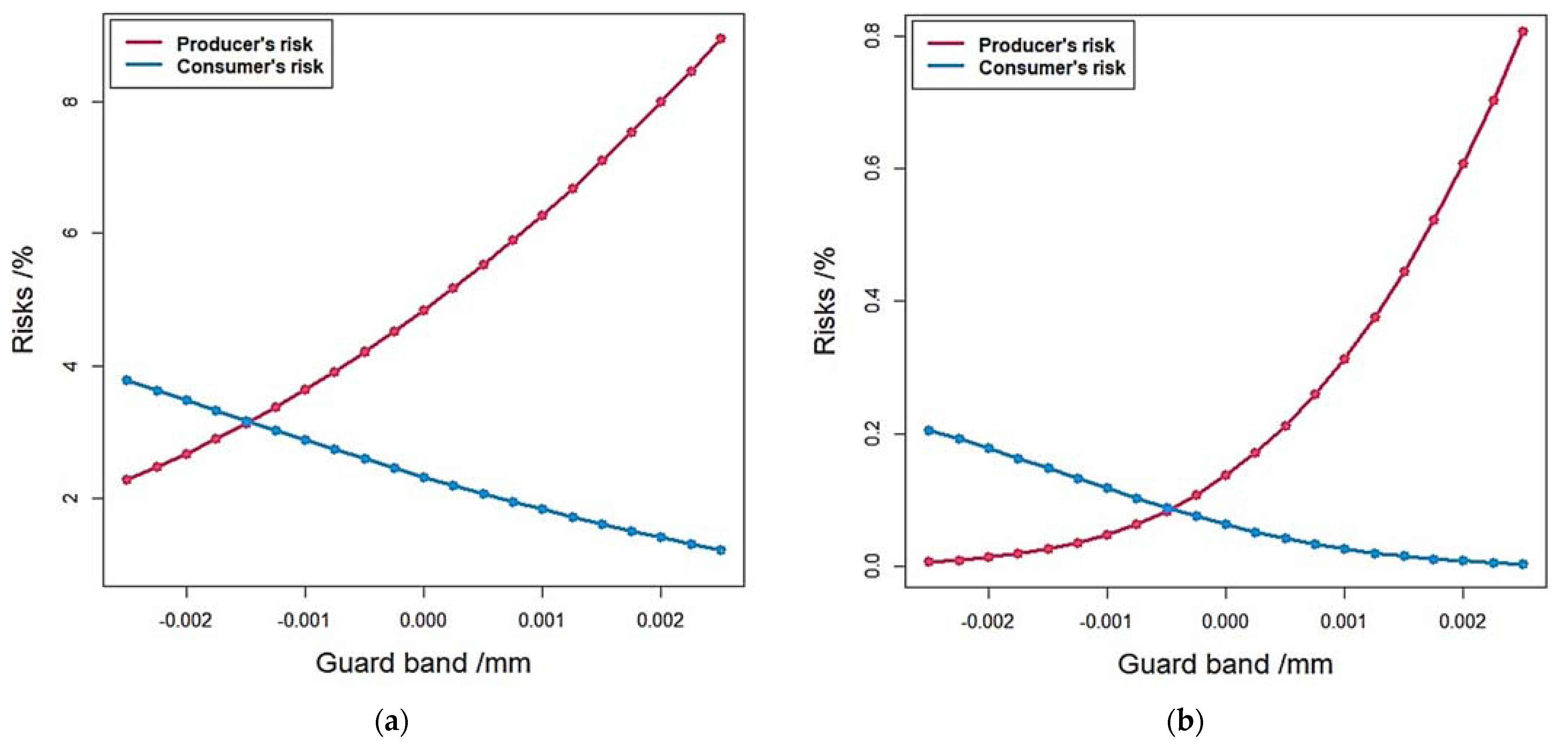
The global producer’s and consumer’s risks of the improved model are lower compared to the initial model (Figure 6).

The values in Figure 6, as well as on all subsequent figures, should be viewed in two directions, regarding the sign of the length of the guard band. Negative values for a guard band in Figure 6 are respective to the model of the minimization of the producer’s risk and refer to the case described in Figure 2a, when the tolerance interval is within the acceptance interval. A smaller negative value represents a wider guard band. If the value of the guard band is equal to zero, the tolerance interval is equal to the acceptance interval, as shown in Figure 2b. Positive values of the guard band correspond to the model of minimization of the global consumer’s risk (Figure 2c). A larger positive value indicates a larger length of the guard band $w$.

Unlike the specific risk, the global risks have different values for the different lengths of the guard band. The global producer’s risk is the lowest in the case when the length of the guard band is $\mathrm{w}=-0.0025$ mm, and the highest if it is $\mathrm{w}=0.0025$ mm (Figure 6a). For the global consumer’s risk, the opposite is true (Figure 6b).

Values for global consumer and producer risk are usually expressed as percentages. Multiplying these probabilities by 10,000 results in the number of falsely accepted and falsely rejected rings per piece. This multiplication has been conducted for simplicity. These values also can be multiplied by 100, 1000, or any other number that represents the daily, weekly, monthly, or yearly production of bearing rings or some other product. The number of falsely accepted and falsely rejected rings is lower in the improved model than in the initial one. The reduction of scrap and, thus, the decrease in production costs for the manufacturer and the reduction of the risk of purchasing rings that do not conform to specifications are shown in

Table 1. Reducing of the number of rings rejected as non-conforming although they meet specifications, and those accepted as conforming, but which do not meet specifications.

Global Risk	$\mathbf{w}=-0.0025\mathbf{mm}$		$\mathbf{w}=0$		$\mathbf{w}=0.0025\mathbf{mm}$
Model	Initial	Improved	Initial	Improved	Initial	Improved
$R_P$	288	0	484	14	895	81
$R_C$	380	21	233	6	122	0

. The number of rings that were falsely accepted or falsely rejected is given per piece. The values are shown for the characteristic lengths of the guard band.

3.2. Metrics Analysis

For basic tested metrics: accuracy, precision, recall and F1 score, the values of the metrics for the improved model are higher in comparison with the values of the metrics in the initial model, (Figure 7).

In the initial model, the accuracy drops along the guard band axis (Figure 7a). For the producer’s risk minimization model with the positive guard band values, the accuracy value drops as the guard band length increases, i.e., the number of rings classified in TP and TN category decreases. For models with negative guard band values, seen from zero to the left side of the graph, with an increase in the length of the guard band, the accuracy increases. That is, the number of rings classified into the TP and TN categories increases. For the improved model, the accuracy metric graph changes behavior in comparison with the initial model. The values of the accuracy metric increase along the guard band axis to the maximum value $accuracy=0.9983486$, and then they fall (Figure 7b). The maximum value is reached when the total number of rings classified in the categories TP and TN is equal to 9984, for the length of the guard band $w=-0.001$ mm. Since the guard band value is negative, this is a producer’s minimization risk model. In that case, the multiplicative factor has a value $r=-0.4.$ Because of measurement uncertainty, there is no perfect classification in metrology, in the sense that all measured values are classified either in the TP or TN category. One of the two values, FA or FR, is always non-zero. If both values were equal to zero at the same time, the absence of measurement uncertainty would be implied, which is not possible. Furthermore, in the conformity assessment process, because of classification in categories, imbalanced data are obtained. For a properly conducted measurement, and controlled manufacturing process, with few products rejected as non-conforming, TP is always much higher than TN. If the number of rings classified as TN is negligible in comparison with the number of rings in the TP category, the accuracy metric is insensitive to the TN category and measures the number of rings classified in the TP category. In that case, it is better to apply some other metric associated with confusion matrices as a measure of the tested model performance [37,38,39]. The classic choices are the precision and recall metrics.

Due to the decrease in global consumer’s risk, the precision curve increases along the guard band axis. According to the definition, precision measures the number of rings that are within the acceptance interval and that are classified in the TP category. In the model of the producer’s risk minimization, this number decreases as the length of the guard band increases. In the consumer’s risk minimization model, the number of such categorized rings increases with the increase in the length of the guard band.

The reverse is true for the recall metric. Since the number of conformed rings classified in the TP category is decreasing, and the global producer’s risk is increasing along the guard band axis, the recall curve falls. Individually by models, for the model of the minimization of global producer’s risk, the recall curve grows while increasing the length of the guard band. In the model of minimizing the consumer’s risk, recall falls. With the improved model, the value of the accuracy is equal to recall for $w=0.0025$ mm. The total number of rings classified into categories TP and TN is then the smallest and amounts to 9919. The value of the multiplicative factor is $r=1.$

The values for the F1 score fall along the guard band axis in both the initial and improved models. The F1 score metric behaves in the same way as accuracy; only the values taken by F1 score are higher compared to accuracy. For the higher positive values of the guard band, accuracy drops faster in comparison with the F1 score. The maximum of the F1 score in the improved model is 0.9991976. The maximum is achieved for the same length of the guard band $w=-0.001$ mm, and the same multiplier $r=-0.4,$ as well as with the accuracy metric. The fact that the F1 score is the harmonic mean of the precision and recall metric is clearly visible in Figure 7. F1 is symmetrically placed between precision and recall. Deviations from symmetry are, at most, of the order of magnitude ${10}^{-3}$ in the initial model, and the order of magnitude ${10}^{-5}$ in the improved model.

The characteristic points on both graphs from Figure 7 are the intersection points of the precision, recall, and F1 score curves. Values of the metrics in the intersection point, in the initial model, are $precision=recall=F1=0.9647,$ and achieve for $w=-0.001475$ mm. In the improved model, the values of the metrics at the point of intersection are equal to $precision=recall=F1=0.9991.$ In this case, the length of the guard band is equal to $w=-0.0004649$ mm.

From Formulas (22)–(24), it is easy to see that $precision=recall=F1$ iff $R_C=R_P.$ This means that the risk curves of the initial and improved models intersect at points with the same values of the guard band $w=-0.001475$ mm and $w=-0.0004649$ mm, respectively, Figure 8.

The corresponding values of the multiplicative factors are $r=-0.59$ for initial model, and $r=-0.18596$ for improved model. In the intersection of the risk curves, the values for the risks of the initial model are equal to $R_C=R_P=3.16\%.$ The values of the risks for the improved model are $R_C=R_P=0.086\%$.

Generally, Formulas (22)–(24) are valid for each model. This means that for each model can be determined the length of the guard band for which the values of the global producer’s and consumer’s risk are equal, and thus the length of the guard band for which the values of the precision, recall, and F1 score are equal.

For data that occur in metrology, it is always true that $TP·TN>FA·FR$. According to [40], it is valid $kappa\le MCC$, which is clearly visible from Figure 9.

It is obtained numerically that, in both the initial and improved model, kappa and MCC curves reach their maximum for $R_C=R_P.$ As with precision, recall, and F1 metrics, when $R_C=R_P,$ it is also worth that is $kappa=MCC.$ The maximums are achieved for the negative values of the guard band, i.e., for the model of minimization of the global producer’s risk. For the initial model, the maximum value is $kappa=MCC=0.662825$ for the length of guard band $w=-0.001475$ mm, and for $r=-0.59.$ With the improved model, the maximum is reached for $w=-0.0004649$ mm and $r=-0.18596$, and it has a value of $kappa=MCC=0.731748.$ Values of these statistics in the range of 0.61–0.80 indicate a moderate level of agreement between actual and predicted results [34].

3.3. Guard Banding by Confusion Matrix

The initial lengths of the guard band are the same for the initial and improved models, but they differ in sign depending on whether it was about minimizing the global risk of the producer or consumer. In this way, it is easier to compare the initial and improved model because the comparison is made in the same nodes of the subdivision of the interval $\left[-1,1\right]$ for the same multiplicative factor $r.$ The highest value of the guard band for the model of minimization of the consumer’s risk, shown in Figure 2c, is set to $w=0.0025$ mm. In the model of minimization of the producer’s risk, this value has a negative sign (Figure 2a). The initial length of the guard band can be larger or smaller than the specified one. In that case, the graphs for the global risk of producers and consumers, and for the selected metrics, will be displayed in a wider or narrower range, respectively. The corresponding values of the calculated risks and metrics will not change if the range of the graphs on the guard band axis is wider. The graphs will only have new values added for the extension points. It can be problematic if a small initial length of the guard band is set. Then, it can occur that characteristic points, such as the intersection of precision, recall, and F1 metrics, are not included in the displayed graph. If it is assumed that such characteristic points exist, it is necessary to increase the initial length of the guard band.

The general question is, what is the optimal length of the guard band? Over the last few decades, many methods and recommendations for guard banding have been developed. In many applications, the length $w$ of the guard band is assumed to be equal to the expanded uncertainty $U$ [41,42]. This means that $w=2u_0=U.$ Based on expanded uncertainty, guard band length can be established so that $w=3U=6u_0$ (6 sigma rule) or $w=1.5U=3u_0$ (3 sigma rule), [4]. A more complicated formula in which the length of the guard band is expressed through an exponential function is detailed in [43]. The length of the guard band can also be calculated using the test of uncertain ratio (TUR) [44,45]. In addition, methods were developed where the acceptance interval was set by means of maximization of the revenue from processes without the systematic effect of measurement uncertainty [46] or with unknown systematic effect, [47]. Recently, methods have been developed to determine the guard band in multivariate models for total risk calculation [48,49]. Furthermore, there is always the opportunity for producers and consumers to compromise and agree on the level of the risks. In that case, it is up to the producer to find the length of the guard for a given consumer risk.

In this paper, the metrics associated with the confusion matrices were used to determine the optimal length $w$ of the guard band. One option is to set the length of the guard band to suit the situation when $R_P=R_C.$ Another option is to take advantage of changes in the behaviour of the Cohen’s kappa and Matthew’s correlation coefficient metrics.

For all the basic tested metrics, the values of the metric for the improved model are higher in comparison to the values of the metrics in the initial model. The only tested metrics that behave differently are kappa and Matthew’s correlation coefficient. There are change points for these two metrics. At these points, the curves of the improved model intersect the curves of the initial model (Figure 9). At the intersection points, the values of the kappa, or MCC metrics, are the same for the initial and improved models. The change point exists both in the producer’s risk minimization model and in the consumer’s risk minimization model. For $wϵ[-0.0025,-0.001548\rangle$ and $wϵ\langle 0.001003,0.0025]$, the kappa statistics of the improved model $kapp{a}_{Im}$ are smaller than the kappa statistics of the initial model $kapp{a}_{In}.$ For $wϵ\left[-0.001548,0.001003\right]$ hold $kapp{a}_{Im}\ge kapp{a}_{In}.$ Analogously, for the MCC statistic, it holds that for $wϵ[-0.0025,-0.001808\rangle$ and for $wϵ\langle 0.001282,0.0025]$ worth $MC{C}_{Im}<MC{C}_{In}.$ For $wϵ\left[-0.001808,0.001282\right]$, it holds that $MC{C}_{Im}\ge MC{C}_{In}.$ For both metrics, the subscript $In$ represents the label for the initial model, and the subscript $Im$ represents the label for the improved model. It naturally arises that it is possible to make use of these changes in the behavior of metrics to determine the optimal length of the guard band. The list of possible values of the guard band, together with the corresponding parameters, is demonstrated in

Table 2. Suggested values of the guard band and associated parameters.

w/mm	Model	Metrics	r	Risks	$\left[{\mathit{A}}_{\mathit{L}},{\mathit{A}}_{\mathit{U}}\right]/\mathbf{mm}$
$-0.001475$	In * Rp_min	$precision=recall=F1=0.9647$ $kappa=MCC=0.662825$	$-0.59$	$R_C=3.16\%$ $R_P=3.16\%$	$\left[99.976525,100.023475\right]$
$-0.0004649$	Im Rp_min	$precision=recall=F1=0.9991$ $kappa=MCC=0.731748$	$-0.18596$	$R_C=0.086\%$ $R_P=0.086\%$	$\left[99.97754,100.0225\right]$
$-0.001548$	In, Im Rp_min	kappaIn = kappaIm = 0.6625	$-0.6192$	$R_C=3.21\%$ $R_P=3.09\%$	$\left[99.976452,100.023548\right]$
$0.001003$	In, Im Rc_min	$kapp{a}_{In}=kapp{a}_{Im}=0.6355$	$0.4012$	$R_C=1.84\%$ $R_P=6.28\%$	$\left[99.979,100.021\right]$
−0.001808	In, Im Rp_min	$MC{C}_{In}=MC{C}_{Im}=0.6614$	$-0.7232$	$R_C=3.36\%$ $R_P=2.85\%$	$\left[99.97619,100.0238\right]$
$0.001282$	In, Im Rc_min	$MC{C}_{In}=MC{C}_{Im}=0.6444$	$0.5128$	$R_C=0.019\%$ $R_P=0.38\%$	$\left[99.97928,100.0207\right]$

* In—initial model, Im—improved model, Rp_min—producer’s risk minimization, Rc_min—consumer’s risk minimization.

.

By comparison of the data from Table 2, it can be concluded that the most favorable situation for minimizing the producer’s risk for the initial model is at the point of change, as $MC{C}_{In}=MC{C}_{Im}=0.6614$. Therefore, the optimal guard band for the initial model in the case of minimizing the global risk of the producer is equal to $w=-0.001808$ mm. In this case, the producer’s risk is the smallest and equal to $R_P=2.85\%,$ but the consumer’s risk is the highest for all proposed lengths of the guard bands. The most favorable situation with the improved model is for $precision=recall=F1=0.9991.$ Then, the producer’s and consumer’s global risk are the smallest and amount to $R_C=R_P=0.086\%.$ Therefore, when minimizing the producer’s risk, in the improved model, it is optimal to set the length of the guard band to $w=-0.0004649$ mm.

In practice, consumer risk minimization models are more common because the manufacturer wants to deliver the highest-quality product to the customer. A low-quality product damages the manufacturer’s reputation and increases its costs due to product returns. For the model of consumer risk minimization, in the initial model, the recommended optimal length of the guard band is $w=0.001282$ mm. This is exactly the length of the guard band for which the MCC curves for the initial and improved model intersect and holds $MC{C}_{In}=MC{C}_{Im}=0.6444.$ This same length of the guard band is the optimal length in the improved model, too. With the consumer risk minimization model, in that case, the global producer’s and consumer’s risks are the lowest and the amounts $R_P=0.38\%$ and $R_C=0.019\%.$

Although the lengths of the guard band are smaller in the intersection points of the kappa metric compared to the values of the guard band in the intersection points of the MCC metric, the optimal is to take the length of the guard band that corresponds to the intersections of the MCC curves, because in that case, the values of the risks are lower. Generally, recent research shows that the MCC metric has better properties than the kappa statistic, [40,50].

In addition, the length of the guard band determined using the new method, based on the intersection points of the MCC curves of the initial and improved models, is smaller than the length of the guard band determined using the standard method based on expanded uncertainty. According to the standard method, it follows from the formula $w=2u_0$ that the length of the guard band for the initial model is $w=0.022$ mm, and for the improved model $w=0.0132$ mm.

All values in Table 2 are obtained numerically, although originally, measurements can be made up to the order of magnitude ${10}^{-7}$ mm, i.e., in 0.1 μm. The values in Table 2, as well as in the text, are intentionally not rounded to make it easier to see the difference between the reference parameters that describe the models.

4. Conclusions

Conformity assessment is a procedure that verifies whether a product meets the required specifications or not. The check is carried out based on measurements with the calculation of the risk of a wrong decision, either that decision refers to accepting a non-conforming product or rejecting a product that conforms to specifications.

Until now, the formulas for calculating the global risk of the producer and the global risk of the consumer have not been observed in the light of machine learning as binary classifiers that can be used to classify products into characteristic categories of confusion matrices. Although in the main document [1] of the International Bureau of Weights and Measures (Bureau International des Poids et Mesures, BIPM) there are examples in which such a classification is partially implemented, the possibility of applying this method is not widely recognized. Classification, unlike machine learning, is performed without the training set and test set based on sample characteristics obtained by measurement, as well as associated measurement uncertainties. Moreover, the method enables the construction of curves for metrics associated with confusion matrices. Using these curves, it is possible to analyze and compare the behavior of the model and determine the optimal length of the guard band.

The characteristic metrics associated with the confusion matrices were used to compare two models for which the conformity of the measured inner diameter of the ring with the given specifications is assessed. Based on the behavior of the MCC metric, it was estimated that it is optimal to set the length of the guard band to the value that corresponds to the point of intersection of the MCC curves of the initial and improved model. Choosing the optimal length of the guard band, and determining the acceptance interval, is based on the condition of achieving the minimal global risk of the producer and consumer. The negative value of the guard band for which $MC{C}_{In}=MC{C}_{Im}$ holds corresponds to the minimization of the global producer’s risk. A positive value of the guard band corresponds to the model of minimization of the global consumer’s risk.

The assessment of global producer’s and consumer’s risk is a method that can be utilized in numerous areas. Combining this method with machine-learning techniques provides a new dimension when evaluating the conformity of products to specified standards. In future work, it remains to be seen how the metrics associated with the confusion matrices behave for centered and non-centered models. It is also necessary to investigate the behavior of metrics with respect to different values of the measurement uncertainties associated with the prior and likelihood function, as well as the behavior of the metrics that were not included in this study.

References

1. BIPM; IEC; IFCC; ILAC; ISO; IUPAC; IUPAP; OIML. Evaluation of Measurement Data—The Role of Measurement Uncertainty in Conformity Assessment, JCGM 106:2012. BIPM. 2012. Available online: https://www.bipm.org/documents/20126/2071204/JCGM_106_2012_E.pdf/fe9537d2-e7d7-e146-5abb-2649c3450b25?version=1.7&t=1659083025736&download=true (accessed on 26 March 2023).
2. Allard, A.; Fischer, N.; Smith, I.; Harris, P.; Pendrill, L. Risk calculations for conformity assessment in practice. In Proceedings of the 19th International Congress of Metrology, Paris, France, 24–26 September 2019. [Google Scholar] [CrossRef]
3. Runje, B.; Horvatić Novak, A.; Razumić, A.; Piljek, P.; Štrbac, B.; Orošnjak, M. Evaluation of Consumer and Producer Risk in Conformity Assessment Decision. In Proceedings of the 30th DAAAM International Symposium “Intelligent Manufacturing & Automation”, Zadar, Croatia, 23–26 October 2019. [Google Scholar] [CrossRef]
4. ILAC-G8:09/2019. Guidelines on Decision Rules and Statements of Conformity. 2019. Available online: https://ilac.org/publications-and-resources/ilac-guidance-series/ (accessed on 18 May 2023).
5. Puydarrieux, S.; Pou, J.M.; Leblond, L.; Fischer, N.; Allard, A.; Feinberg, M.; El Guennouni, D. Role of measurement uncertainty in conformity assessment. In Proceedings of the 19th International Congress of Metrology, Paris, France, 24–26 September 2019. [Google Scholar] [CrossRef]
6. Dias, F.R.S.; Lourenço, F.R. Measurement uncertainty evaluation and risk of false conformity assessment for microbial enumeration tests. J. Microbiol. Methods 2021, 189, 106312. [Google Scholar] [CrossRef]
7. Bettencourt da Silva, R. Eurachem/CITAC Guide: Setting and Using Target Uncertainty in Chemical Measurement. 2015. Available online: https://www.eurachem.org/index.php/publications/guides/gd-stmu (accessed on 18 May 2023).
8. Pendrill, L.R. Using measurement uncertainty in decision-making and conformity assessment. Metrologia 2014, 51, 3206. [Google Scholar] [CrossRef]
9. Williams, A.; Magnusson, B. Eurachem/CITAC Guide: Use of Uncertainty Information in Compliance Assessment. 2021. Available online: https://www.eurachem.org/index.php/publications/guides/uncertcompliance (accessed on 18 May 2023).
10. EUROLAB Technical Report, No. 1/2017-Decision Rules Applied to Conformity Assessment. Available online: https://www.eurolab.org/pubs-techreports (accessed on 18 May 2023).
11. Lira, I. A Bayesian approach to the consumer’s and producer’s risks in measurement. Metrologia 1999, 36, 397. [Google Scholar] [CrossRef]
12. Toczek, W.; Smulko, J. Risk Analysis by a Probabilistic Model of the Measurement Process. Sensors 2021, 21, 2053. [Google Scholar] [CrossRef] [PubMed]
13. Separovic, L.; de Godoy Bertanha, M.L.; Saviano, A.M.; Lourenço, F.R. Conformity Decisions Based on Measurement Uncertainty—A Case Study Applied to Agar Diffusion Microbiological Assay. J. Pharm. Innov. 2020, 15, 110–115. [Google Scholar] [CrossRef]
14. BIPM; IEC; IFCC; ILAC; ISO; IUPAC; IUPAP; OIML. Evaluation of Measurement Data—Supplement 1 to the “Guide to the Expression of Uncertainty in Measurement”—Propagation of Distributions Using a Monte Carlo Method, JCGM 101:2008. BIPM. 2008. Available online: https://www.bipm.org/documents/20126/2071204/JCGM_101_2008_E.pdf/325dcaad-c15a-407c-1105-8b7f322d651c?version=1.12&t=1659082897489&download=true (accessed on 26 March 2023).
15. Božić, D.; Runje, B. Selection of an Appropriate Prior Distribution in Risk Assessment. In Proceedings of the 33rd International DAAAM Virtual Symposium “Intelligent Manufacturing & Automation”, Vienna, Austria, 26–27 October 2022. [Google Scholar] [CrossRef]
16. Pennecchi, F.R.; Kuselman, I.; Di Rocco, A.; Brynn Hibbert, D.; Sobina, A.; Sobina, E. Specific risks of false decisions in conformity assessment of a substance or material with a mass balance constraint—A case study of potassium iodate. Measurement 2021, 173, 108662. [Google Scholar] [CrossRef]
17. Separovic, L.; Bettencourt da Silva, R.J.N.; Lourenço, F.R. Determination of intrinsic and metrological components of the correlation of multiparameter products for minimising the risks of false conformity decisions. Measurement 2021, 180, 109531. [Google Scholar] [CrossRef]
18. Separovic, L.; Lourenço, F.R. Measurement uncertainty and risk of false conformity decision in the performance evaluation of liquid chromatography analytical procedures. J. Pharm. Biomed. Anal. 2019, 171, 73–80. [Google Scholar] [CrossRef]
19. Lombardo, M.; Margueiro da Silva, S.; Lourenço, F.R. Conformity assessment of medicines containing antibiotics—A multivariate assessment. Regul. Toxicol. Pharmacol. 2022, 136, 105279. [Google Scholar] [CrossRef]
20. Kuselman, I.; Pennecchi, F.; Bettencourt da Silva, R.J.N.; Brynn Hibbert, D. Conformity assessment of multicomponent materials or objects: Risk of false decisions due to measurement uncertainty—A case study of denatured alcohols. Talanta 2017, 164, 189–195. [Google Scholar] [CrossRef] [PubMed]
21. de Oliveira, E.C.; Lourenço, F.R. Risk of false conformity assessment applied to automotive fuel analysis: A multiparameter approach. Chemosphere 2021, 263, 128265. [Google Scholar] [CrossRef] [PubMed]
22. Pennecchi, F.R.; Kuselman, I.; Di Rocco, A.; Brynn Hibbert, D.; Semenova, A.A. Risks in a sausage conformity assessment due to measurement uncertainty, correlation and mass balance constraint. Food Control 2021, 125, 107949. [Google Scholar] [CrossRef]
23. Božić, D.; Samardžija, M.; Kurtela, M.; Keran, Z.; Runje, B. Risk Evaluation for Coating Thickness Conformity Assessment. Materials 2023, 16, 758. [Google Scholar] [CrossRef]
24. Brandão, L.P.; Silva, V.F.; Bassi, M.; de Oliveira, E.C. Risk Assessment in Monitoring of Water Analysis of a Brazilian River. Molecules 2022, 27, 3628. [Google Scholar] [CrossRef] [PubMed]
25. Caelen, O. A Bayesian interpretation of the confusion matrix. Ann. Math Artif. Intell. 2017, 81, 429–450. [Google Scholar] [CrossRef]
26. Grandini, M.; Bagli, E.; Visani, G. Metrics for Multi-Class Classification: An Overview. arXiv 2020. [Google Scholar] [CrossRef]
27. Jiao, Y.; Du, P. Performance measures in evaluating machine learning based bioinformatics predictors for classifications. Quant. Biol. 2016, 4, 320–330. [Google Scholar] [CrossRef]
28. Luque, A.; Carrasco, A.; Martín, A.; de las Heras, A. The impact of class imbalance in classification performance metrics based on the binary confusion matrix. Pattern Recognit. 2019, 91, 216–231. [Google Scholar] [CrossRef]
29. Jeni, L.A.; Cohn, J.F.; De La Torre, F. Facing Imbalanced Data-Recommendations for the Use of Performance Metrics. In Proceedings of the International Conference on Affective Computing and Intelligent Interaction (ACII), Geneva, Switzerland, 2–5 September 2013. [Google Scholar] [CrossRef]
30. Flach, P.A.; Lachiche, N. Naive Bayesian Classification of Structured Data. Mach. Learn. 2004, 57, 233–269. [Google Scholar] [CrossRef]
31. Tharwat, A. Classification assessment methods. Appl. Comput. Inform. 2021, 17, 168–192. [Google Scholar] [CrossRef]
32. Alvarez, S.A. An Exact Analytical Relation among Recall, Precision, and Classification Accuracy in Information Retrieval. Technical Report BC-CS-2002-01. Available online: http://www.cs.bc.edu/~alvarez/APR/aprformula.pdf (accessed on 19 May 2023).
33. Flach, P.; Kull, M. Precision-recall-gain curves: PR analysis done right. Adv. Neural. Inf. Process. Syst. 2015, 28, 838–846. Available online: https://proceedings.neurips.cc/paper/2015/file/33e8075e9970de0cfea955afd4644bb2-Paper.pdf (accessed on 19 May 2023).
34. McHugh, M.L. Interrater reliability: The kappa statistic. Biochem. Med. 2012, 22, 276–282. [Google Scholar] [CrossRef]
35. Chicco, D.; Tötsch, N.; Jurman, G. The Matthews correlation coefficient (MCC) is more reliable than balanced accuracy, bookmaker informedness, and markedness in two-class confusion matrix evaluation. BioData Min. 2021, 14, 13. [Google Scholar] [CrossRef] [PubMed]
36. Chicco, D.; Jurman, G. The advantages of the Matthews correlation coefficient (MCC) over F1 score and accuracy in binary classification evaluation. BMC Genom. 2020, 21, 6. [Google Scholar] [CrossRef] [PubMed]
37. Juba, B.; Le, H.S. Precision-Recall versus Accuracy and the Role of Large Data Sets. In Proceedings of the 33rd AAAI Conference on Artificial Intelligence, Honolulu, HI, USA, 27 January–1 February 2019. [Google Scholar] [CrossRef]
38. Sun, Y.; Wong, A.K.C.; Kamel, M.S. Classification of imbalanced data: A review. Intern. J. Pattern Recognit Artif. Intell. 2009, 23, 687–719. [Google Scholar] [CrossRef]
39. Tanha, J.; Abdi, Y.; Samadi, N.; Razzaghi, N.; Asadpour, M. Boosting methods for multi-class imbalanced data classification: An experimental review. J. Big Data 2020, 7, 70. [Google Scholar] [CrossRef]
40. Delgado, R.; Tibau, X.-A. Why Cohen’s Kappa should be avoided as performance measure in classification. PLoS ONE 2019, 14, e0222916. [Google Scholar] [CrossRef] [PubMed]
41. Volodarsky, E.T.; Kosheva, L.O.; Klevtsova, M.O. The Role Uncertainty of Measurements in the Formation of Acceptance Criteria. In Proceedings of the XXIX International Scientific Symposium “Metrology and Metrology Assurance” (MMA), Sozopol, Bulgaria, 6–9 September 2019. [Google Scholar] [CrossRef]
42. Haloulos, I.; Theodorou, D.; Zannikou, Y.; Zanninkos, F. Monitoring fuel quality: A case study for quinizarin marker content of unleaded petrol marketed in Greece. Accred. Qual. Assur. 2016, 21, 203–210. [Google Scholar] [CrossRef]
43. Dobbert, M.A. Guard-Band Strategy for Managing False-Accept Risk. NCSLI Meas. 2008, 4, 44–48. [Google Scholar] [CrossRef]
44. Deaver, D. Guardbanding with Confidence. In Proceedings of the NCSL Workshop and Symposium, Chicago, IL, USA, 1 September 1994; Available online: https://download.flukecal.co/pub/literature/ddncsl94.pdf (accessed on 24 May 2023).
45. Purata-Sifuentes, O.-J.; Hernández-Balandrán, L.-E.; Tornero-Navarro, M.-G. Role of the measurement uncertainty in cone penetration test results of lubricating grease. In Proceedings of the Joint IMEKO TC11 & TC24 hybrid conference, Dubrovnik, Croatia, 16–20 October 2022. [Google Scholar] [CrossRef]
46. Shirono, K.; Tanaka, H.; Koike, M. Economic optimization of acceptance interval in conformity assessment: 1. Process with no systematic effect. Metrologia 2022, 59, 045005. [Google Scholar] [CrossRef]
47. Shirono, K.; Tanaka, H.; Koike, M. Economic optimization of acceptance interval in conformity assessment: 2. Process with unknown systematic effect. Metrologia 2022, 59, 045006. [Google Scholar] [CrossRef]
48. Margueiro da Silva, C.; Lourenço, F.R. Definition of multivariate acceptance limits (guard-bands) applied to pharmaceutical equivalence assessment. J. Pharm. Biomed. Anal. 2023, 222, 115080. [Google Scholar] [CrossRef] [PubMed]
49. Bettencourt da Silva, R.J.N.; Lourenço, F.; Brynn Hibbert, D. Setting Multivariate and Correlated Acceptance Limits for Assessing the Conformity of Items. Anal. Lett. 2022, 55, 2011–2032. [Google Scholar] [CrossRef]
50. Chicco, D.; Warrens, M.J.; Jurman, G. The Matthews Correlation Coefficient (MCC) is More Informative Than Cohen’s Kappa and Brier Score in Binary Classification Assessment. IEEE Access 2021, 9, 78368–78381. [Google Scholar] [CrossRef]
Figure 1. An example of a situation where the measured value has a high measurement uncertainty whose value exceeds the lower limit of the tolerance interval [4]. The symbols T L and T U in figures are marks for the lower and upper limits of the tolerance interval, respectively.
Applsci 13 08187 g001
Figure 2. A different relationship between acceptance interval and tolerance interval: (a) Model of the producer’s risk minimization; (b) Shared risk; (c) Model of the consumer’s risk minimization. The symbols A L and A U in figures are marks for the lower and upper limits of the acceptance interval, respectively.
Applsci 13 08187 g002
Figure 3. Initial measurement system.
Applsci 13 08187 g003
Figure 4. New automated measurement system. Different stages of the automated measurement process.
Applsci 13 08187 g004
Figure 5. Confusion matrix.
Applsci 13 08187 g005
Figure 6. Initial versus improved model: (a) Global producer’s risk; (b) Global consumer’s risk.
Applsci 13 08187 g006
Figure 7. Basic metrics curves: (a) Initial model; (b) Improved model.
Applsci 13 08187 g007
Figure 8. Intersections of the risk curves: (a) Initial model; (b) Improved model.
Applsci 13 08187 g008
Figure 9. Kappa and MCC statistics for initial and improved model.
Applsci 13 08187 g009