FMGAN: A Filter-Enhanced MLP Debias Recommendation Model Based on Generative Adversarial Network

Abstract

In recommendation models, bias can distort the distribution of user-generated data, leading to inaccurate representation of user preferences. Failure to filter out biased data can result in significant learning errors, ultimately reducing the accuracy of the recommendation model. To address this issue, this paper proposes a Generative Adversarial Network (GAN) model comprising a filter-enhanced Multi-Layer Perceptron (MLP) generator and a linear discriminator to mitigate bias and improve the accuracy of the recommendation. The proposed model leverages the GAN architecture, where the filter structure in the generator enhances the data distribution before model training, allowing for the generation of more precise recommendation lists. The discriminator learns from the skew-corrected user review list to extract user features, which are then used alongside the recommendation list generated by G in an adversarial process. This adversarial process enables each component to optimize and improve itself while strengthening the correction effect. To enhance the accuracy of G generation, we evaluate the influence of three different input lists on the filter effect. Finally, we validate our model on two real-world datasets by comparing the effect of filter-augmented MLP and pure MLP generators. Our results demonstrate the effectiveness of filters, and our model achieves better recommendation accuracy than other baseline models.

1. Introduction

Information retrieval systems play a vital role in information dissemination and filtering. These systems encompass a range of applications, such as web search [1], recommendation systems [2], personalized advertisements [3], and text retrieval [4]. An accurate and efficient recommendation system can mitigate the effects of information overload by providing users with a curated list of relevant content that aligns with their query conditions [5], thereby greatly improving the user experience. Collaborative filtering (CF) [6] recommendation is commonly used in recommendation systems. CF generates representation vectors of users and items by learning user history interaction information, and calculates the similarities and associations between users and items based on the representation vectors. CF has shown excellent performance in generating personalized recommendations, but the computational complexity of CF increases as the system grows. Handling large datasets and computing similarity measures can become challenging and affect the algorithm’s scalability. Recently, the graph convolutional neural network [7] has become the state-of-the-art method in the recommendation problem. This method has a strong ability to process structured data. A well-designed graph convolutional model can learn correlations of different data sources and high-order information. However, the graph convolutional neural network model is usually not easy to construct suitable graph nodes and edges, and the design of the network structure is also relatively complicated. It is also necessary to use more side information in the dataset to extract features.

No matter what method is applied for recommendation, it needs to learn from the user’s historical interaction information. Obtaining user history interaction information for the recommendation process can be challenging as it is typically generated during the user’s usage and not collected through questionnaires [8]. There are several ways to collect data for recommendation models. One common approach is to obtain specific evaluations of items from users, display these evaluations, and create a user–item index in the evaluation matrix. Another method that aligns better with modern software operation is to collect implicit feedback, where a user’s click on an item is considered a positive evaluation, and non-clicked items are treated as negative evaluations. Implicit feedback data are collected easily, and there is a greater abundance of interaction information than with explicit feedback.

When users rely on software to make decisions, the collected data may be influenced by a range of factors such as exposure, conformity, and location, resulting in data deviations. Exposure bias, for instance, arises when users are only exposed to specific items, and position bias is formed because users tend to interact more with items placed in front. These deviations cause the interaction distribution of users and items to deviate from their real preference distribution [9], thereby affecting the recommendation model’s input. Consequently, it becomes challenging for the model to learn user preferences from noisy data. For example, when using implicit feedback data, treating all uninteracted items as negative feedback can create exposure bias. In such cases, the recommendation model may fail to analyze items similar to the user’s favorite item $i$, which they have not yet observed. To address this problem, evaluation indicators such as the propensity score method [10] or sampling methods [11] can be employed to mitigate exposure bias. By using these methods, the likelihood of exposure bias can be reduced, and the model can learn user preferences more accurately.

User interaction with information is a spontaneous behavior, resulting in limited amounts of data collected, reflected in a list of interaction histories of varying lengths. Inconsistent data lengths can lead to inconsistencies in the training format of the recommendation system, making it difficult to extract user and item features using a collaborative method. This challenge has been partially resolved by applying vector training approaches in various recommender methods. This approach combines a user’s preferences for items into a vector, unifying the training format, which is the natural input format for neural networks. Different network layers can be used to address the problem of large differences in historical interaction data [12]. Filter-enhanced Multi-Layer Perceptron (MLP) is a novel data processing module in the network form, originally used for signal processing by blocking signals of specific frequencies and allowing signals of other frequencies to pass. In the recommendation models, it can be used as a learnable and efficient noise reduction method incorporated into the network to further enhance the recommendation system’s efficiency.

In order to overcome the noise caused by the deviation in the collected data and the data length inconsistency in the user interaction information, this paper proposes a filter-enhanced Multi-Layer Perceptron recommendation model based on the Generative Adversarial Network (GAN) framework. Firstly, a generative adversarial model is constructed using the GAN architecture, consisting of a generator G and a discriminator D. G generates fake user interaction lists by learning from the real data distribution, while D distinguishes between the probability of user interaction lists coming from real data versus generated lists. Once the model converges, G generates high-confidence recommendations for specific users. Secondly, to better extract user preferences from historical data, G converts users and items into latent vectors and applies filters to remove noise from the information in order to achieve the debias effect. Multiple linear layers are then utilized to increase the model’s fitting nonlinearity data capabilities, thereby improving convergence. D also utilizes multi-linear layers to process the data. Lastly, the study compared three different conditional vectors to determine the optimal model input.

The major contributions of this paper are summarized as follows:

(1)

We proposed a filter-enhanced MLP recommendation model based on the Generative Adversarial Network framework to solve the problem of recommendation bias. Through comparisons of two real-world datasets from Movielens and Ciao, we demonstrated the effectiveness of filter-enhanced MLP to improve data partitioning to address recommendation bias and achieve better results compared to baseline models.

(2)

We designed three different condition vectors to enhance the learning ability of the model and verified the influence of different condition vectors on the model effect through experimental comparison.

This paper is structured as follows. Section 2 provides an overview of the key related work. In Section 3, we present our proposed model, detailing its design and implementation. Section 4 presents the experimental results of our model on two real-world datasets from Movielens and Ciao, comparing the performance to that of the baseline models. Finally, Section 5 concludes the paper by summarizing our findings and outlining areas for future research.

2. Related Work

2.1. Model-Based Collaborative Filtering

Among various collaborative filtering recommendation systems, model-based collaborative filtering has emerged as the most effective method for efficiently extracting user representation vectors [13]. This type of recommendation system builds a model to learn a user’s past preferences for items and stores this information in various ways. When the user requests recommendation information, the model calculates the required information. Matrix factorization (MF) is the most popular model, where a matrix is constructed to represent a user’s historical interactions, with the rows representing the user index, the columns representing the item index, and the values representing the user’s preference for the item [14]. MF learns from this matrix, with items being linearly linked to provide recommendation results. Model-based recommendation systems encompass a range of methods, including PMF [15] for click rate prediction, BPR [16], and FISM [17] for TOP-N prediction. Recently, DNN-based models have attracted significant attention [18]. The powerful nonlinear fitting capability of DNNs enables them to fit any continuous function that describes the relationship between users and items. DNN-based models include AutoRec [19] for click rate prediction and NCF [20] for TOP-N recommendation. The collaborative recommendation filtering system based on cognitive similarity is famous for its efficient extraction of user item similarity. Nguyen et al. [21] proposed a three-layer structure that can extract cognitive similarity, which can accurately identify neighbors and improve algorithm consistency.

2.2. Debias Methods

Exposure bias can be debiased during the evaluation process or model training. The deviation correction method in the evaluation process includes the inverse properisty score [22] method, which reduces the weight of items with high frequency of occurrence and increases the weight of items with low frequency of occurrence during the evaluation process. This method is also applicable to selection bias. There are many debias methods in the model training process, including the confidence weight method, such as WMF [23], and the exposure-based recommendation model, such as EXMF [24]. Sampling-based methods use a sampling strategy to specify which samples are used to update the recommended model parameters. For example, NCF applies uniform negative sampling through neural network models.

Recently, a debias method based on invariant learning [25] has achieved great success. The focus of this method is to separate various influencing factors in the recommendation process and find out the most important influencing factors for learning. InvPref [26] separates environmental factors and user preference factors. In InvCF [27], the influencing factors of popularity bias are decomposed into preference factors and popularity factors, the preference and popularity encoders are optimized through joint training, and only the preference factors are applied in the recommendation process, so the deviation correction is achieved by isolating the popularity factors. Invariant learning not only needs to accurately analyze the influencing of bias factors but also needs to preprocess datasets to obtain the data of influencing factors, such as user popularity ranking, item location, and other information. In the joint learning process, it is necessary to design the learning method and parameter list reasonably to achieve the best recommendation effect.

2.3. Generative Adversarial Network and GAN-Based Recommendation

Ian Goodfellow proposed a novel approach called Generative Adversarial Network (GAN) [28], which was initially applied in image generation and achieved significant success [29]. The GAN architecture comprises a generator G, a discriminator D, and adversarial learning between them. G generates fake data by learning real data, and its objective is to produce synthetic data that is as close as possible to real data. D distinguishes between real and fake data and aims to accurately differentiate the two. The adversarial learning process of G and D in GAN can be viewed as a max–min game, where G continually generates more accurate data through learning to reduce the probability of D identifying real data, while D continuously learns to increase the difference between real and fake data, improving its ability to distinguish between them. After adversarial learning, G can learn to capture the ideal distribution of users and generate credible recommendation results that differ from real data. GAN has not only been successful in image generation but has also found applications in other domains, such as WaveGAN [30] for music generation and SeqGAN [31] for sentence generation.

IRGAN [32] is an information retrieval system that combines recommendation systems, web search, question answering systems, and GAN. In the domain of recommendation systems, IRGAN employs GAN architecture where the generator G aims to produce item IDs that match the user’s preferences, and the discriminator D estimates the probability of an item ID originating from real interaction data or being generated by G. The IRGAN method has successfully applied the GAN framework to the recommender system field, and its effectiveness has led to further developments.

One such development is the CFGAN [33,34] model, which employs a vector training method instead of the pointwise [35] training method used in IRGAN. Vector data have several inherent advantages, such as richer and more complete user features and their compatibility with neural network input patterns. Additionally, updating network parameters with stochastic gradient descent is feasible with vector data. In CFGAN, the user interaction vector ${\mathit{r}}_{\mathit{u}}$ and random noise vector ${\mathit{c}}_{\mathit{u}}$ are used as inputs to the generator, which directly generates the user interaction vector ${\widehat{\mathit{r}}}_{\mathit{u}}$, represented as an n-dimensional sparse vector. Unlike IRGAN, D evaluates the given vector as the user’s history interaction vector ${\mathit{r}}_{\mathit{u}}$, rather than calculating the probability that G generates the interaction vector ${\widehat{\mathit{r}}}_{\mathit{u}}$. While the original GAN model is primarily applied to dense data, the data in the recommendation system are often sparse due to data collection issues. CFGAN utilizes binary implicit feedback vectors, where 1 denotes user interaction with the item, and 0 denotes no interaction. However, this type of bias data may cause G to generate an unhelpful output consisting of all 1s.

To address the bias issue, CFGAN proposes three solutions, including zero-reconstruction (ZR), partial-masking (PM), and a combination of both methods (ZP). The ZR method integrates the G-generated list with real interactions for MSE loss calculation, mitigating overfitting. The PM method incorporates negative sampling into each user’s training process. Specifically, a mask vector ${\mathit{k}}_{\mathit{u}}$ is formed by randomly selecting a certain number of items, and an n-dimensional indicator vector ${\mathit{e}}_{\mathit{u}}$ is generated to represent user u’s interaction with item i. By adding ${\mathit{e}}_{\mathit{u}}$ and ${\mathit{k}}_{\mathit{u}}$ and multiplying the resulting vector elementwise with the user’s historical interaction data, a new interaction vector is generated, achieving the desired sampling effect. Negative sampling enables the model to learn more diverse user preferences, thereby improving its ability to analyze the optimal state and overcome exposure bias. However, frequent item selection during training leads to high computational complexity in the model calculation process. Finally, the objective function of G in CFGAN is expressed as a combination of the adversarial loss, reconstruction loss, and regularization term, expressed as:

$$\begin{array}{c}{J}^G={\displaystyle \sum }_u\left(log\left(1-D\left({\widehat{\mathit{r}}}_{\mathit{u}}\odot \left({\mathit{e}}_{\mathit{u}}+{\mathit{k}}_{\mathit{u}}\right)|{\mathit{c}}_{\mathit{u}}\right)\right)+\alpha \cdot {\displaystyle \sum }_j{\left(x_{uj}-{\widehat{x}}_{uj}\right)}^2\right)\end{array}$$

(1)

where ${\mathit{k}}_{\mathit{u}}$ is the mask vector of the PM method, $\alpha$ denotes the hyperparameter for MSE loss, $x$ is the value in $\widehat{\mathit{r}}$, and $\widehat{x}$ is 0. On the other hand, D aims to maximize the classification accuracy between the generated user interaction vector ${\mathit{r}}_{\mathit{u}}$ and the real interaction vector ${\mathit{r}}_{\mathit{u}}$. The objective function of D is:

$$\begin{array}{c}{J}^D=-{\displaystyle \sum }_u\left(logD\left({\mathit{r}}_{\mathit{u}}|{\mathit{c}}_{\mathit{u}}\right)+log\left(1-D\left(\left({\widehat{\mathit{r}}}_{\mathit{u}}\odot {\mathit{e}}_{\mathit{u}}\right)|{\mathit{c}}_{\mathit{u}}\right)\right)\right)\end{array}$$

(2)

where ${\mathit{e}}_{\mathit{u}}$ is the indicator vector in Formulas (1) and (2) and $\odot$ denotes elementwise multiplication in the vector. To accommodate vector data as the input, CFGAN employs a neural network model that is well-suited for vectors, with both the generator and discriminator implemented using multi-layer perceptrons.

2.4. Filter-Enhanced Recommendation

The Filter-enhanced [36] paper proposes a novel neural network structure that incorporates learnable filters and MLP blocks to improve the performance of the network. Filters are commonly used in digital signal processing to selectively modify certain aspects of a signal by adjusting the frequency response, such as high-pass filtering or low-pass filtering. Unlike traditional filtering methods that operate in the time domain, the proposed network converts the input sequence into the frequency domain using the discrete Fourier transform (DFT) before filtering. For a given input sequence $\left\{x_n\right\}$ where $n\in \left[0,N-1\right]$, the DFT is defined by the following formula:

$$\begin{array}{cc}{X}_k={\displaystyle {\displaystyle \sum }_{n=0}^{N-1}}{x}_n{e}^{-\frac{2\pi i}{N}nk},\hfill & \hfill 0\le k\le N-1\end{array}$$

(3)

where $i$ is the imaginary unit, and $X_k$ represents the frequency spectrum of the sequence $\left\{x_n\right\}$ at frequency $\omega =2\pi k/N$. After filtering, the filtered signal can be restored to a real vector $\left\{{\widehat{x}}_n\right\}$ through inverse Fourier transform (IDFT), which converts the signal back from the frequency domain to the time domain:

$$\begin{array}{c}{\widehat{x}}_n=\frac{1}{N}{\displaystyle {\displaystyle \sum }_{k=0}^{N-1}}{X}_k{e}^{\frac{2\pi i}{N}nk}\end{array}$$

(4)

The application of filters to the user’s historical data can mitigate the issue of exposure bias. As a result, the filtered data ${\widehat{x}}_n$ contain more effective information and less noise, leading to more accurate feature extraction by subsequent MLP models. Effective utilization of the filter module can facilitate the generation of superior recommendation results by the recommendation model.

2.5. Analytical Summary of the Literature

The traditional CF model is simple to calculate, but the learning ability of the model will be slightly weak when the amount of data is too large. A graph convolutional neural network can effectively improve learning ability, but it is challenging to construct proper graph nodes and edges. Model learning ability affects the recommendation effect, and the bias in the dataset also affects the recommendation effect. Traditional debias methods need to design complex weight systems or use complex probability calculations to solve specific bias types. Generative Adversarial Networks can automatically optimize the recommendation list through adversarial learning. Different implementation methods of the generator and discriminator bring differentiated recommendation results. Therefore, our target is to design a recommendation model based on a Generative Adversarial Network with strong learning ability and general debias ability.

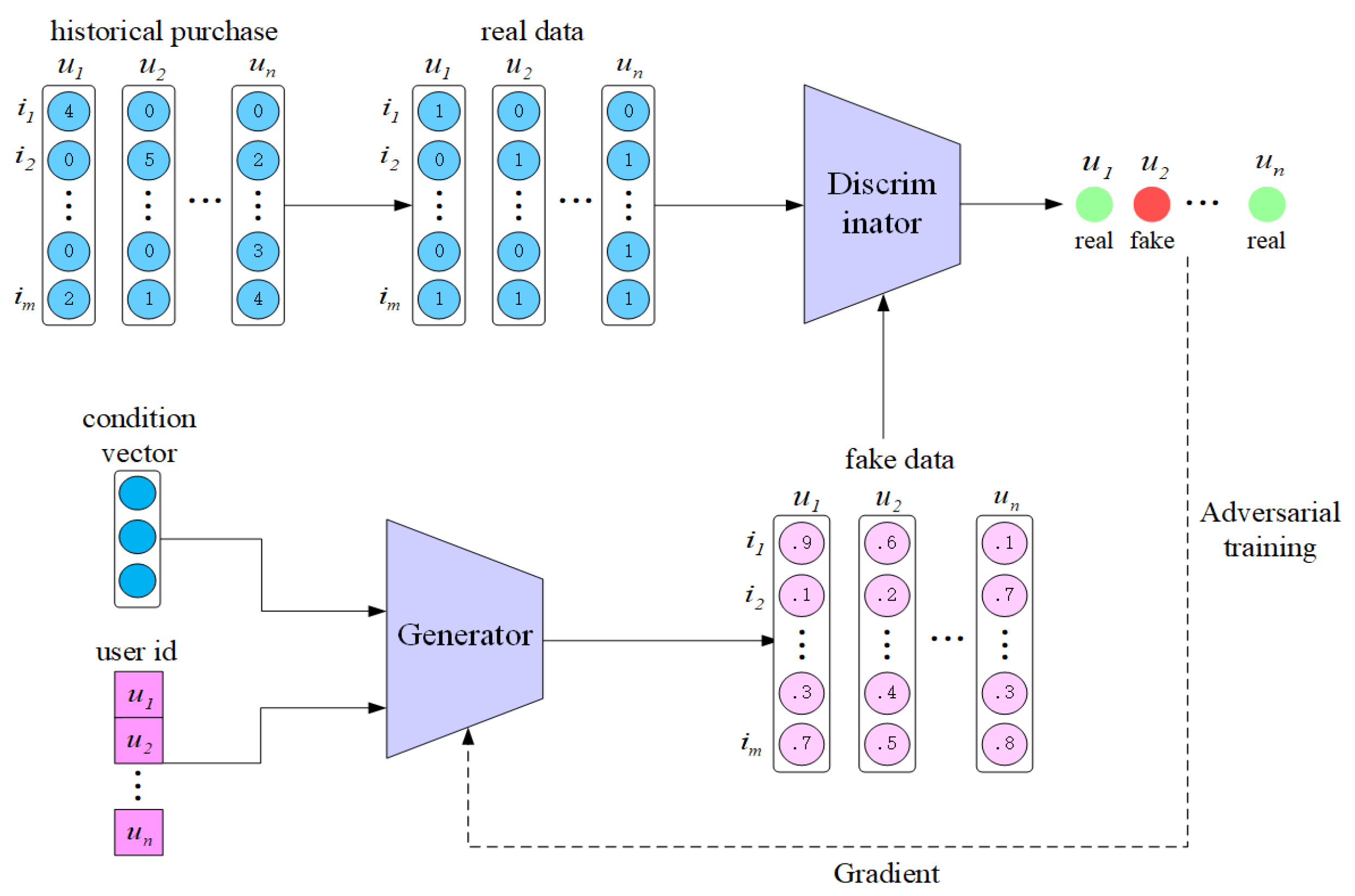
3. Methodology

This paper introduces a novel recommender model that leverages a GAN-based model comprising a filter-enhanced Multi-Layer Perceptron (MLP) generator and a linear discriminator. Figure 1 provides an overview of the proposed approach. Our system takes a user’s interaction history data (consisting of $n$ users and $m$ items per user), a condition vector, and a user ID as inputs. The generator and discriminator are trained using an adversarial approach to learn user preferences and generate top-N recommendations. The following sections delve into the specific details of the generator, discriminator, and the adversarial training process.

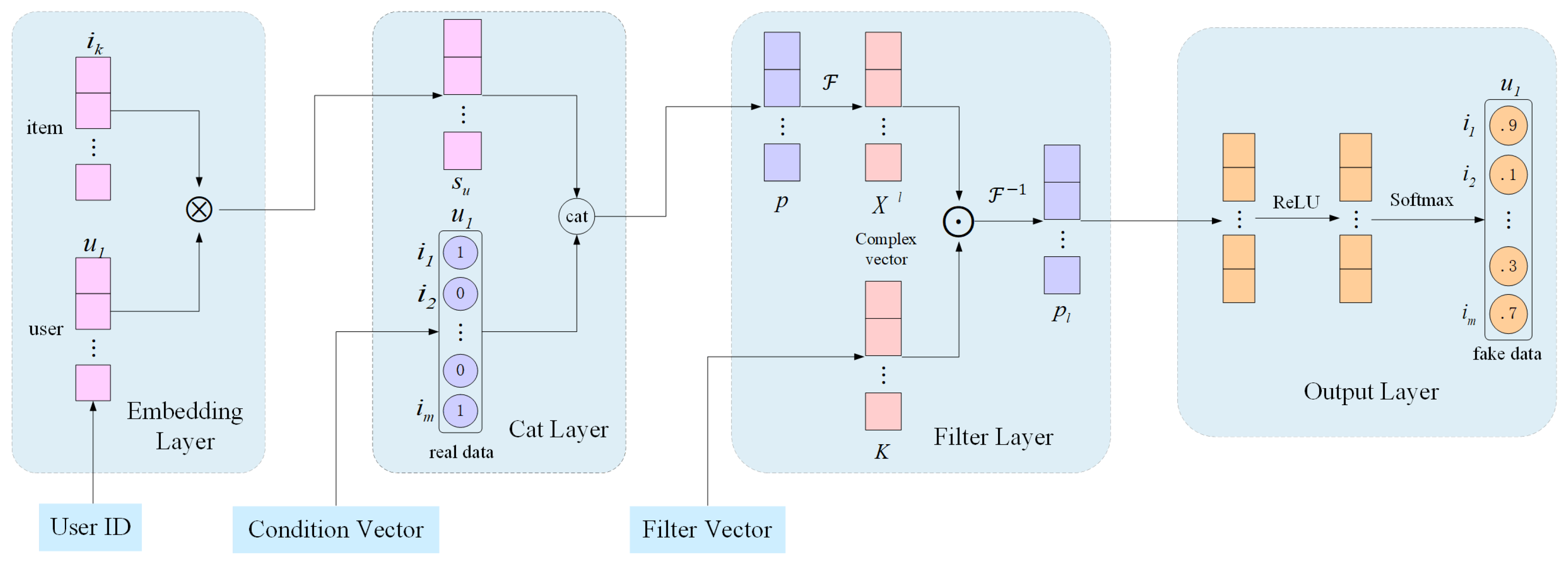
3.1. Generator

The purpose of the generator is to generate a top-N recommendation list based on the user’s historical interaction and user characteristics. Figure 2 illustrates the structure of our generator, which mainly includes input, embedding layer, combination layer, filter layer, and output layer. We will introduce the role of each layer in detail.

The input of G consists of two parts. One is the user ID used to obtain the user embedding vector, and the other is the conditional vector $\mathit{c}$ related to the historical interaction. The embedding vector is used to save the user’s basic preferences and demographic information. The embedding vector provides the generator with stable characteristics of the user, maintaining the basic learning ability of the model. The conditional vector $\mathit{c}$ is an important point of model input. The introduction of this vector is to solve the problem of exposure bias in the recommendation process. This vector can be obtained from historical implicit interaction data or by sampling methods such as negative sampling. The conditional vector provides the generator with short-term preferences of users and alleviates exposure bias, and the two-part input enables G to float up and down around stable features of users to improve recommendation performance. The embedding layer obtains the embedding vectors of users and items by querying user IDs: $U_{embd}=\left\{u_1,u_2,\cdots ,u_d\right\},I_{embd}=\left\{i_1,i_2,\cdots ,i_d\right\}$, where $d$ represents the embedding dimension. The combination layer first calculates the user’s stable feature: ${\mathit{s}}_{\mathit{u}}=U^T\times I$, and concatenates ${\mathit{s}}_{\mathit{u}}$ and the conditional vector $\mathit{c}$ to form the user’s initial preference $\mathit{p}=cat\left({\mathit{s}}_{\mathit{u}},\mathit{c}\right)\in {ℝ}^{1\times 2m}$. $\mathit{p}$ can be directly input into the linear layer, giving a recommendation list, but it consists of two parts. ${\mathit{s}}_{\mathit{u}}$ is the calculation data, and $\mathit{c}$ is collected through real-world user feedback; directly inputting into the linear layer will mix the noise of the two, making the noise further amplified. So, we apply a filter layer in the generator, which can better fuse information and remove part of the noise. The initial preference $\mathit{p}$ is first transformed to the frequency domain by fast Fourier transform:

$$\begin{array}{c}{\mathit{X}}^{\mathit{l}}=ℱ\left(\mathit{p}\right)\in {ℂ}^{1\times m}\end{array}$$

(5)

where $ℱ(\cdot )$ represents the one-dimensional fast Fourier transform, and ${\mathit{X}}^{\mathit{l}}$ is a complex vector representing the spectrum of $\mathit{p}$. This way, we can start the filtering (modulation) operation by multiplying the learnable filter $\mathit{K}\in {ℂ}^{1\times m}$ with ${\mathit{X}}^{\mathit{l}}$ to get the modulated vector $\tilde{\mathit{X}}$:

$$\begin{array}{c}\tilde{\mathit{X}}=\mathit{K}\odot {\mathit{X}}^{\mathit{l}}\in {ℂ}^{1\times m}\end{array}$$

(6)

where $\odot$ represents elementwise multiplication. The filter $\mathit{K}$ is a randomly initialized complex vector. During training, its parameters are updated through the gradients of the optimization function. Following modulation, the resulting vector $\tilde{\mathit{X}}$ remains in the complex domain, necessitating conversion back to the time domain prior to further processing.

$${\mathit{p}}_{\mathit{l}}=\begin{array}{c}{ℱ}^{-1}\left(\tilde{\mathit{X}}\right)\end{array}$$

(7)

where ${ℱ}^{-1}(\cdot )$ represents the inverse Fourier transform. After the last transformation, the initial user preference $\mathit{p}$ has been fused and denoised, resulting in a complete user preference vector ${\mathit{p}}_{\mathit{l}}$ that is suitable for subsequent processing.

The final layer in the neural network architecture consists of two linear layers and an activation function, which are responsible for generating the output. Upon completion of the computation, the data contained in the list are transformed into a probability distribution through the application of the softmax function. This output layer effectively captures the non-linear preferences of the user, ultimately yielding a list of ratings for the items:

$$\begin{array}{c}\widehat{\mathit{r}}=\mathrm{Softmax}\left(\left(ReLU\left({\mathit{p}}_{\mathit{l}}{\mathit{W}}_{\mathbf{1}}+b_1\right)\right){\mathit{W}}_{\mathbf{2}}+b_2\right)\end{array}$$

(8)

where ${\mathit{W}}_{\mathbf{1}},b_1,{\mathit{W}}_{\mathbf{2}},b_2$ are trainable parameters. So far, the generator has generated a list of scores for user $u$, which will serve as input for the discriminator during subsequent adversarial training as fake data. This approach leverages the feedback loop between the generator and discriminator to improve the quality of the generated outputs.

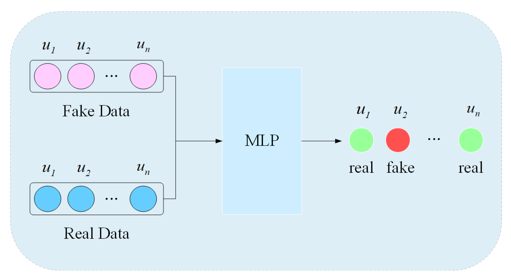
3.2. Discriminator

The primary objective of the discriminator is to assess the likelihood that a given rating list originates from real data, as opposed to fake data. As depicted in Figure 3, the discriminator structure differs from that of the generator, as it solely outputs floating-point numbers representing the probabilities. This probability value serves as a reference point for the generator to refine its output during the adversarial training, thereby facilitating mutual progression. The discriminator comprises an input layer, a data combination layer, and an output layer that includes a linear discriminator. The input layer consists of two real vectors with a length of m, the user real data $\mathit{r}$, and the fake data $\widehat{\mathit{r}}$. These vectors are concatenated to form the input vector $\overline{\mathit{r}}$ for the discriminator. The linear discriminator is then utilized for training and output. An output value close to 0 indicates that the list was likely generated by the generator, while an output value close to 1 indicates that it is more likely to be the user’s historical interaction data. The output layer includes two linear layers and two activation functions, as expressed below:

$$\begin{array}{c}o=sigmoid\left(ReLU\left(\overline{\mathit{r}}{\mathit{W}}_{\mathbf{1}}+b_1\right){\mathit{W}}_{\mathbf{2}}+b_2\right)\end{array}$$

(9)

where $o$ is the output of the discriminator, and ${\mathit{W}}_{\mathbf{1}},b_1,{\mathit{W}}_{\mathbf{2}},b_2$ are trainable parameters.

3.3. Adversarial Training

In the GAN framework, the generator and the discriminator engage in an adversarial training process where the generator generates samples, and the discriminator evaluates their realism by assigning a probability value. This iterative process provides improvement directions for both the generator and the discriminator and is considered the most important aspect of GAN training. During the early stages of training, the generator’s sample distribution can differ significantly from the historical interaction data used by the discriminator, leading to high confidence discrimination and subsequent loss feedback to the generator. The generator then uses this loss as guidance to improve its model parameters and generate more realistic data lists. This cyclic process of generating and confronting continues, leading to mutual progress between the two structures.

The adversarial training process begins by iterating the discriminator on real data and fake data generated by the generator. The discriminator learns the distribution of real data, assigns a loss value, and then learns the distribution of fake data generated by the generator and assigns another loss value. The objective function of the discriminator can thus be expressed as:

$$\begin{array}{c}{J}^D=\underset{\theta }{\min }-{\displaystyle \sum }_u\left(logD\left(\mathit{r}\right)+log\left(1-D\left(G(u|\mathit{c}\right)\right)\right)\end{array}$$

(10)

where $\mathit{r}$ is the historical interaction data, and $\mathit{c}$ is the condition vector.

With each iteration of the adversarial training process, the discriminator improves its discriminatory ability against the generator. The next step involves iterating the generator. The generator generates fake data and then computes the mean squared error (MSE) loss against real data:

$$\begin{array}{c}los{s}_{MSE}=\frac{1}{m}{\left({\widehat{\mathit{r}}}_{\mathit{u}}-{\mathit{r}}_{\mathit{u}}\right)}^2\end{array}$$

(11)

The mean squared error (MSE) loss enables the generator to learn directly from the gap between its generated data and real data; this loss prevents the score generated by G from being too large, as the loss calculated by D is usually small. Excessive generation errors are not easy to be optimized by small discrimination errors. Otherwise, there is a danger of overfitting. The generator’s fake data are then input into the discriminator, which assigns another loss value. This loss serves as a guide for further training and pushes the generated data towards a direction that is more difficult for the discriminator to distinguish, creating an adversarial effect. The adversarial loss can be expressed as:

$$\begin{array}{c}los{s}_{adv}={\displaystyle \sum }_{u}log\left(1-D\left(G\left(u|\mathit{c}\right)\right)\right)\end{array}$$

(12)

The objective function of the generator can then be determined according to the two losses as:

$$\begin{array}{c}\begin{array}{c}{J}^G=\underset{\varphi }{\min }{\displaystyle \sum }_u\left(los{s}_{adv}+\alpha los{s}_{MSE}\right)\end{array}\end{array}$$

(13)

where α is a hyperparameter. The adversarial training process involves the two modules improving each other, leading to healthy progress. The generator improves its embedding vector and generates a high-quality recommendation list that better captures the user’s preferences. The discriminator initially distinguishes real and fake data but may not be robust to noisy data. It continuously searches for small differences between real and fake data to guide the generator towards the desired target through these slight differences. This iterative process helps both modules improve and achieve better results.

3.4. FMGAN Recommendation

During the recommendation process, we use a given user ID and its historical interaction data and index the items that the user has interacted with. Once the model converges, we can perform the prediction process, which involves: (1) analyzing and extracting the user’s characteristics and preferences from their historical interaction data using the model; (2) storing this information in the embedding vectors of users and items; and (3) inputting the user’s information into the model when a recommendation is needed, which then generates an exclusive item recommendation list based on probability.

4. Experiment and Discussion

In the experimental part, we test the effectiveness of the model on two real-world datasets from Movielens and Ciao. Based on the experiments, we will answer the following questions:

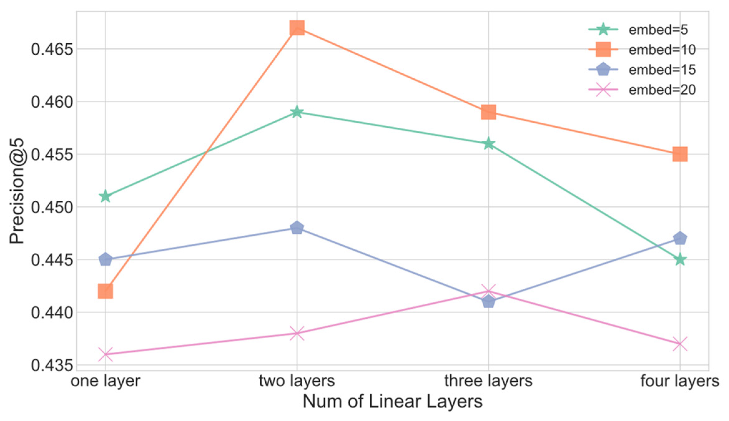
• Effect of embedding dimensions and linear layers.
• Effect of the filter.
• Model performance under different condition vectors.
• Performance comparison of the model with other benchmark models.

4.1. Experiment Setup

4.1.1. Datasets

Our study utilizes two real-world datasets: Movielens 100k/1M and Ciao [37]. For the Ciao dataset, we use the high sparsity version from CFGAN [33]. Both datasets consist of user ID, item IDs, and user ratings for items.

Table 1. The overview of datasets.

Statics	Movielens 100K	Movielens 1M	Ciao
users	943	6039	996
items	1682	3883	1927
ratings	100,000	1,000,209	18,648
sparsity	93.69%	95.72%	99.03%

presents an overview of the datasets’ statistics, wherein explicit ratings of 1–5 points are assigned by users. To convert explicit ratings to implicit ratings, we apply a scoring threshold of 3 points, wherein ratings greater than or equal to 3 points are considered positive evaluations and recorded as 1 in the interaction list. On the other hand, ratings lower than 3 points are recorded as 0. The interaction list generated is used as the condition vector of the generator in our experiments.

4.1.2. Evaluation Metrics

Our research employs four widely used evaluation metrics in top-N recommendation models, namely precision at N (P@N) [38], recall at N (R@N) [39], normalized discounted cumulative gain at N (NDCG@N) [40], and mean reciprocal rank at N (MRR@N) [41]:

$$Precision@\mathrm{N}=\frac{\left|G\left(u\right){\displaystyle \cap }R\left(u\right)\right|}{\left|G\left(u\right)\right|}$$

(14)

$$Recall@\mathrm{N}=\frac{\left|G\left(u\right){\displaystyle \cap }R\left(u\right)\right|}{\left|R\left(u\right)\right|}$$

(15)

$$NDCG@\mathrm{N}=\frac{DCG@\mathrm{N}}{IDCG@\mathrm{N}}=\frac{{{\displaystyle \sum }}_{i=1}^{\mathrm{N}}\frac{1}{{\log }_2\left(i+1\right)}}{{{\displaystyle \sum }}_{i=1}^{\left|ITEM\right|}\frac{1}{{\log }_2\left(i+1\right)}}$$

(16)

$$MRR@\mathrm{N}=\frac{1}{\mathrm{N}}{\displaystyle \sum }_{i=1}^{\mathrm{N}}\frac{1}{ran{k}_i}$$

(17)

In the evaluation formulas, $\mathrm{N}$ represents the length of the recommendation list. In P@N, G(u) denotes the set of items recommended by the generator for user $u$, while R(u) represents the set of items that the user has previously interacted with. In MRR@N, $ran{k}_i$ represents the position of the first relsevant result in the i-th query. P@N measures the proportion of correctly recommended items in the top-N positions, while NDCG@N and MRR@N evaluate the accuracy of the ranking position of relevant items in the recommendation list. Specifically, NDCG@N measures the quality of the position arrangement of all relevant items in the top-N list, while MRR@N assesses the accuracy of the position arrangement of the first relevant item in the top-N positions.

4.1.3. Implementation Details

The experimental settings and parameter selection in our study are as follows: During the training phase, we randomly select 80% of the data in the dataset as the training set, while the remaining 20% of the data are used as the test set. We implement the model with Pytorch in our experiments. The settings and hyperparameters of the model are shown in

Table 2. Model settings and hyperparameters for FMGAN.

FMGAN Model Settings and Hyperparameters
Dataset	$\mathit{\alpha }$	lr	Hidden Layers	First Layer Input Size	Activation Function	Second Layer Input Size	Embedding Dimension	Batch Size
Movielens 100K	0.3	1 × 10−4	2	3306	ReLU	1983	10	64
Movielens 1M	0.3	3 × 10−4	2	7364	ReLU	4418	10	128
Ciao	0.3	7 × 10−5	2	2694	ReLU	1616	10	64

. In addition, G and D are optimized by the Adam algorithm, and the training ratio of G and D is set to 1:1. After the model converges, we compare it with the benchmark model based on P@N, R@N, NDCG@N, and MRR@N, where N is set to 5 and 20.

4.2. Discussion and Results

4.2.1. Effect of Embedding Dimensions and Linear Layers

To begin with, we assess the impact of user and item embedding dimensions, as well as the number of linear layers, on the performance of the generator. The embedding dimension determines the fundamental information learned by the generator. A dimension that is too small is not conducive to maintaining the basic capabilities of the generator, while one that is too large can impede the dynamic learning ability of the generator. The linear layer acts as an operation following the filter, and the combination of multiple linear layers can learn non-linear features and preserve the generator’s output. Figure 4 displays the top five recommendation results of our model, based on the MovileLens100k dataset, for four embedding dimensions and four linear layer numbers. Our generator achieves optimal performance with an embedding dimension of 10 and two linear layers. As the embedding dimension ranges from 5 to 15, performance gradually declines with increasing linear layers. For embedding dimensions of 10 and 20, performance trends consistently, but performance is superior for an embedding dimension of 10.

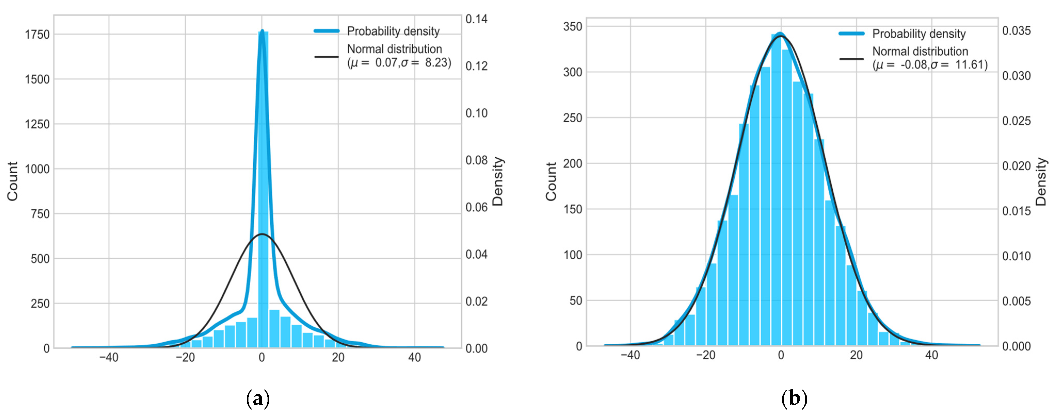
4.2.2. Effect of the Filter

Figure 5 illustrates the data distribution in the generator before the MLP extracts user information. Figure 5a displays the data distribution in the user’s initial preference vector. The figure reveals that the vector comprises nearly 1750 values concentrated around 0 and displays the characteristics of a peaked and thick-tailed distribution, which differs from the normal distribution fitting curve of the same data. This observation indicates that the model’s analysis of the user’s initial preference is biased towards the items the user has interacted with in the past, i.e., those items exposed to the user, which cannot mitigate the impact of exposure bias. Conversely, Figure 5b presents the data distribution in the filtered user preference vector. Notably, the figure does not exhibit any apparent high points, and the data conform closely to a normal distribution fitting curve that is similar to the distribution of the same data. Therefore, the use of such user preference data enables the subsequent MLP module to prioritize more interactive items, provide users with additional recommendation options, and effectively mitigate exposure bias.

The generator leverages filters for bias reduction and information combination to efficiently extract user information. However, increasing the structure also escalates computational complexity. To validate the filter structure’s effectiveness, we train a G and D consisting of a pure MLP network.

Table 3. Performance comparison of FMGAN-im and MLP on Movielens 100K/1M and Ciao.

Datasets	Model	Prec@5	Recall@5	NDCG@5	MRR@5
Movielens 100K	FMGAN-im	0.467	0.154	0.496	0.698
	MLP	0.421	0.139	0.449	0.657
Movielens 1M	FMGAN-im	0.435	0.110	0.458	0.650
	MLP	0.402	0.101	0.425	0.629
Ciao	FMGAN-im	0.070	0.081	0.092	0.153
	MLP	0.061	0.071	0.086	0.146

displays the results. The evaluation reveals that our model performs better, demonstrating that incorporating filters enhances the model’s efficacy.

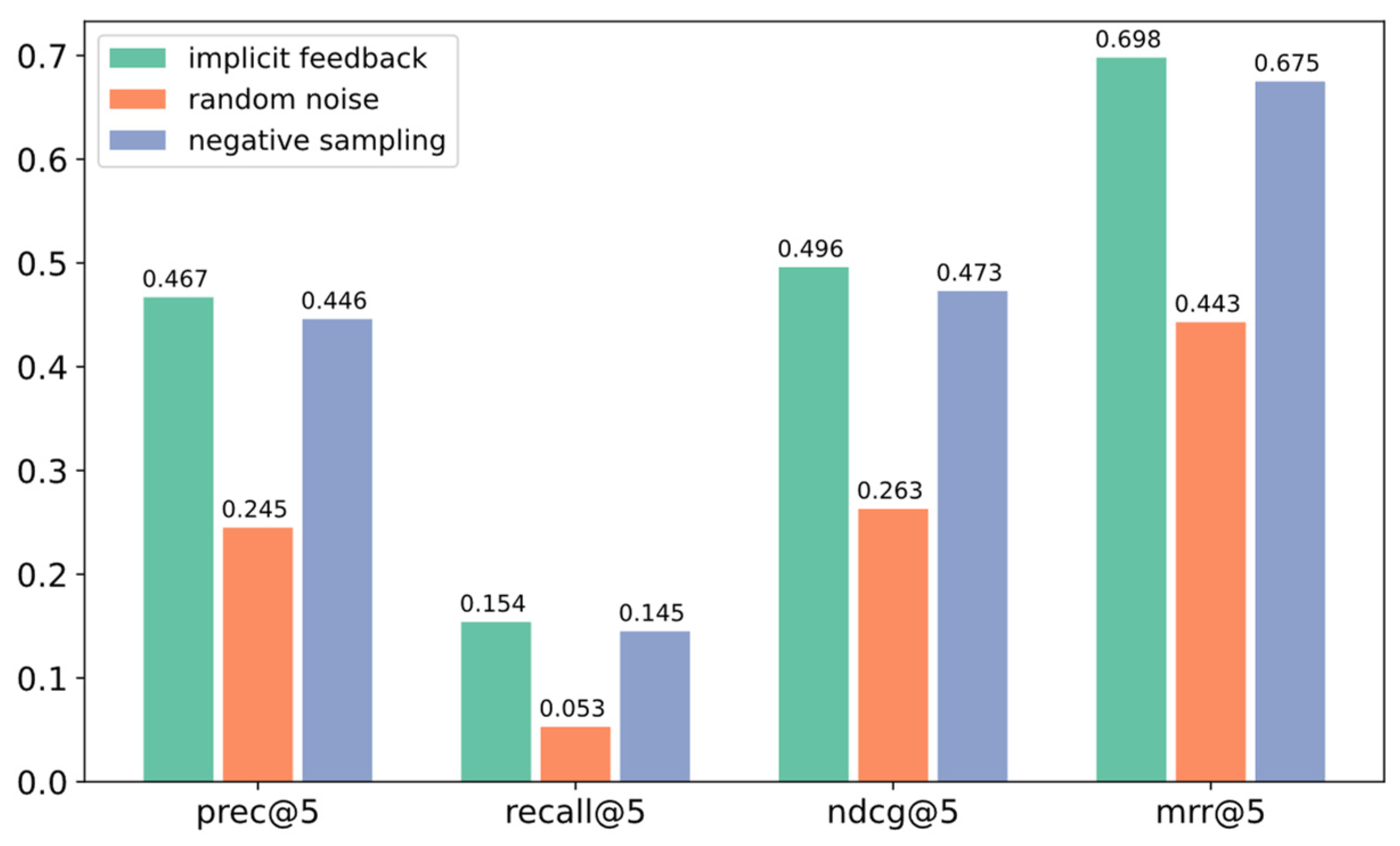
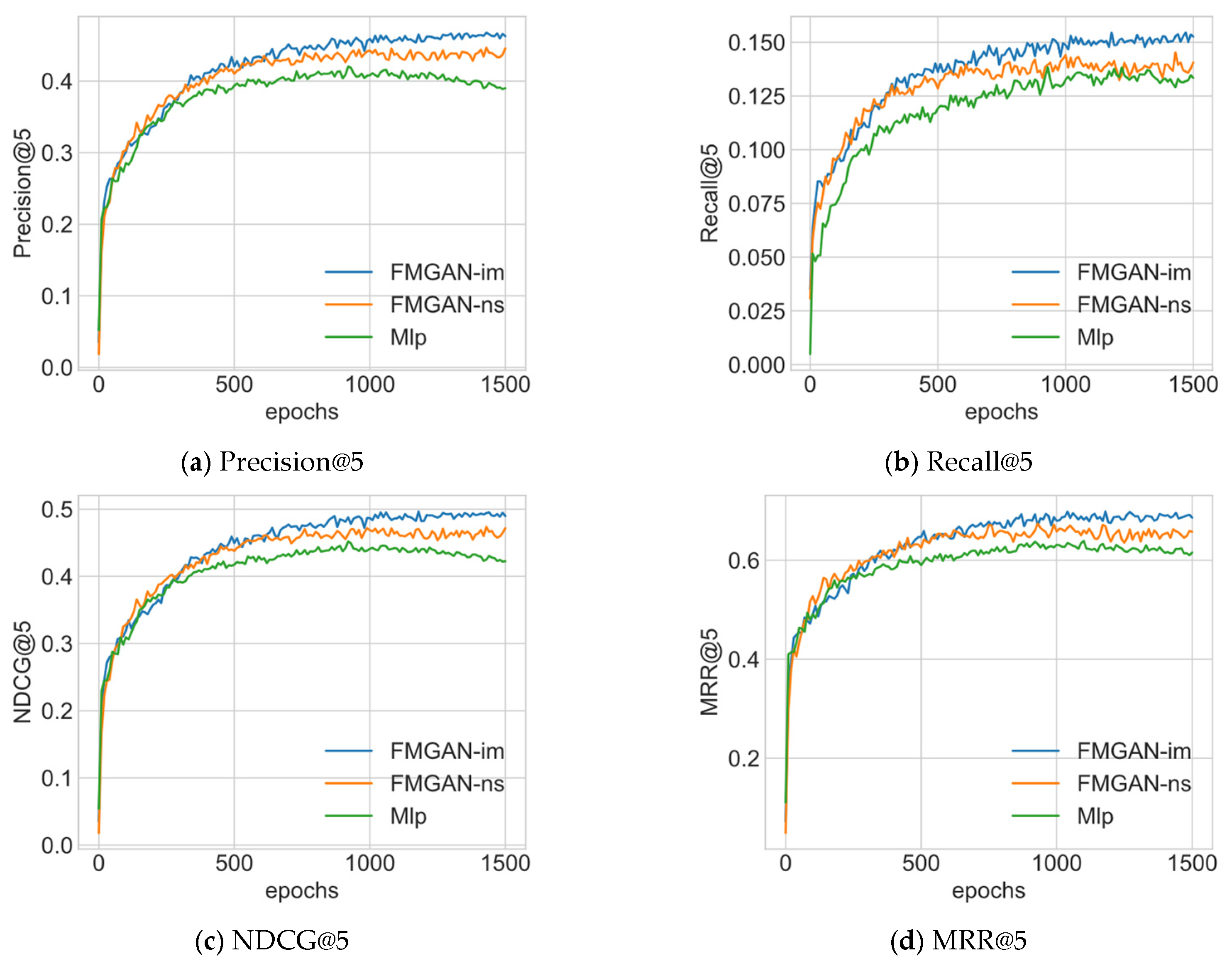
4.2.3. Model Performance under Different Condition Vectors

The generator’s generation process involves a condition vector c, which is selected as the user’s interaction list in the paper, termed FMGAN-im (Implicit feedback). However, c can take various forms, such as using a random noise vector (random noise). FMGAN-ns (negative sampling) employs the negative sampling method to generate a pseudo-interaction list by randomly selecting some uninteracted items. Noise vectors are generated via uniform sampling with a length equal to the number of items. In negative sampling, a certain proportion (0.8 times the number of items in this paper) of uninteracted item subscripts is sampled with uniform probability, and the user interaction data (i.e., 0, 1) of these subscripts are extracted as a pseudo-interaction list. The results are presented in Figure 6. It is apparent that using random noise vectors yields poor results because the filter structure used in this study truncates the noise vectors, resulting in similar filtered vector distributions, making it difficult for each user to distinguish their respective characteristics, thereby deteriorating the recommendation effect. The model employs the negative sampling list as the condition vector, which yields satisfactory results. However, it uses a portion of the data for training, and multiple random selections lack substantial user bases. During the generator’s training process, random sampling is necessary for each iteration, and the computation cost varies. Hence, it is not employed as the final condition vector in this study.

Figure 7 illustrates the Learning trend of FMGAN-im, FMGAN-ns, and MLP on Movielens 100K. The upward trend of both models is similar, but our model can continue improving for an extended period to achieve superior results. Furthermore, the training epoch does not significantly increase, and the degree of computational complexity remains acceptable.

Finally, to validate the efficacy of our model, we compare it with the baselines in the top-N recommendation task. The baseline models are defined as follows:

• ItemPop: A model that uses the most purchase records for recommendation, which is the simplest non-personalized algorithm method.
• BPR: The model pairs purchased items with unpurchased items and optimizes the correct ranking order between item pairs.
• FISM: The model uses two low-latitude latent vectors to simulate the item–item similarity matrix.
• IRGAN: The model applies the GAN architecture to the recommendation system and uses the binary classification loss to train point states or point pairs. This method is specifically introduced in Section 2.2.
• CFGAN: Improves the use of vectors as training parameters and introduces a sampling method to improve the training process. This method is specifically introduced in Section 2.2.

Table 4. Performance comparison results in Movielens 100K.

Metrics	P@5	P@20	R@5	R@20	G@5	G@20	M@5	M@20
ItemPop	0.182	0.139	0.105	0.253	0.165	0.196	0.255	0.293
BPR	0.350	0.237	0.117	0.288	0.372	0.381	0.558	0.575
FISM	0.428	0.285	0.146	0.354	0.464	0.429	0.675	0.686
IRGAN	0.320	0.223	0.110	0.278	0.346	0.370	0.539	0.525
CFGAN	0.445	0.327	0.149	0.360	0.477	0.440	0.682	0.701
FMGAN-ns	0.446	0.330	0.145	0.359	0.473	0.437	0.675	0.698
FMGAN-im	0.467	0.340	0.154	0.365	0.496	0.454	0.698	0.719

,

Table 5. Performance comparison results in Movielens 1M.

Metrics	P@5	P@20	R@5	R@20	G@5	G@20	M@5	M@20
ItemPop	0.155	0.120	0.075	0.195	0.153	0.179	0.251	0.296
BPR	0.340	0.251	0.075	0.207	0.347	0.361	0.535	0.554
FISM	0.419	0.304	0.106	0.269	0.442	0.398	0.635	0.649
IRGAN	0.262	0.213	0.071	0.165	0.265	0.245	0.302	0.337
CFGAN	0.431	0.307	0.107	0.164	0.452	0.404	0.643	0.659
FMGAN-ns	0.433	0.308	0.106	0.162	0.451	0.402	0.641	0.654
FMGAN-im	0.435	0.311	0.110	0.169	0.458	0.406	0.650	0.662

and

Table 6. Performance comparison results in Ciao.

Metrics	P@5	P@20	R@5	R@20	G@5	G@20	M@5	M@20
ItemPop	0.030	0.023	0.039	0.126	0.046	0.063	0.054	0.067
BPR	0.035	0.024	0.040	0.140	0.050	0.065	0.067	0.079
FISM	0.060	0.037	0.071	0.179	0.080	0.110	0.127	0.147
IRGAN	0.034	0.022	0.042	0.110	0.045	0.065	0.080	0.087
CFGAN	0.068	0.040	0.079	0.190	0.089	0.117	0.151	0.164
FMGAN-ns	0.065	0.039	0.076	0.186	0.087	0.113	0.149	0.163
FMGAN-im	0.070	0.043	0.081	0.192	0.092	0.120	0.153	0.166

present the performance of the baseline model and our model on two real-world datasets. Based on the experimental results, our model outperforms other baselines on both datasets and has achieved remarkable enhancements on the Movielens 100k dataset. The results of the high sparsity Ciao dataset shown in Table 6 are very noteworthy. Although it has a similar number of users and items to the Movielens 100k dataset, the scarcity of interaction records greatly reduces the recommendation performance. Comparing it with the baseline model indicates that the GAN model architecture can be effectively applied in the recommendation system field, and the generator’s combination of filters and MLP can efficiently extract user preference information.

The above experimental results show that the improvement of our model has achieved certain results. The model generates embedding vectors based on user and item IDs to store the information representation learned by the model. After improving the data distribution through filters, MLP can generate recommendation lists more accurately. The introduction of GAN architecture helps the model strengthen this learning process. The introduction of different input vectors expands the structure of the model and provides more directions for future improvement.

5. Conclusions

In this paper, we provide an analysis of several approaches to address the bias problem in recommender systems and propose our filter-enhanced MLP recommendation model based on the GAN framework. The use of the GAN framework in image processing has paved the way for its application in recommendation models, with IRGAN and CFGAN being early examples. Building on these models, we further expand the generator and employ a model composed of filters and MLP blocks to generate recommendation lists. Selecting historical interaction data on the conditional vector proves to be effective, as there is no need for negative sampling during each training epoch. We evaluate our model on two real-world datasets from Movielens and Ciao, fine-tune the model parameters, test the model under different conditional vectors, and demonstrate the effectiveness of the filter through comparison with the pure MLP model. Our model outperforms other models in the top-N recommendation task.

In future work, we aim to investigate alternative sampling methods [42,43] to replace the conditional vector to enhance the model’s robustness and explore the utilization of additional user demographic information to provide more references for the model training process.

References

- Burges, C.; Shaked, T.; Renshaw, E.; Lazier, A.; Deeds, M.; Hamilton, N.; Hullender, G. Learning to rank using gradient descent. In Proceedings of the 22nd International Conference on Machine Learning, Bonn, Germany, 7–11 August 2005; pp. 89–96. [Google Scholar]
- Koren, Y.; Bell, R.; Volinsky, C. Matrix factorization techniques for recommender systems. Computer 2009, 42, 30–37. [Google Scholar] [CrossRef]
- Qin, T.; Liu, T.-Y.; Xu, J.; Li, H. LETOR: A benchmark collection for research on learning to rank for information retrieval. Inf. Retr. 2010, 13, 346–374. [Google Scholar] [CrossRef]
- Adomavicius, G.; Tuzhilin, A. Toward the next generation of recommender systems: A survey of the state-of-the-art and possible extensions. IEEE Trans. Knowl. Data Eng. 2005, 17, 734–749. [Google Scholar] [CrossRef]
- Liu, T.-Y. Learning to rank for information retrieval. Found. Trends® Inf. Retr. 2009, 3, 225–331. [Google Scholar] [CrossRef]
- Ekstrand, M.D.; Riedl, J.T.; Konstan, J.A. Collaborative filtering recommender systems. Found. Trends® Hum. Comput. Interact. 2011, 4, 81–173. [Google Scholar] [CrossRef]
- Gao, C.; Wang, X.; He, X.; Li, Y. Graph neural networks for recommender system. In Proceedings of the Fifteenth ACM International Conference on Web Search and Data Mining, Tempe, AZ, USA, 21–25 February 2022; pp. 1623–1625. [Google Scholar]
- Zhao, Z.; Chen, J.; Zhou, S.; He, X.; Cao, X.; Zhang, F.; Wu, W. Popularity Bias Is Not Always Evil: Disentangling Benign and Harmful Bias for Recommendation. arXiv 2021, arXiv:2109.07946. [Google Scholar] [CrossRef]
- Zhou, Y.; Xu, J.; Wu, J.; Taghavi, Z.; Korpeoglu, E.; Achan, K.; He, J. PURE: Positive-Unlabeled Recommendation with Generative Adversarial Network. In Proceedings of the 27th ACM SIGKDD Conference on Knowledge Discovery & Data Mining, Singapore, 14–18 August 2021; pp. 2409–2419. [Google Scholar]
- Schnabel, T.; Swaminathan, A.; Singh, A.; Chandak, N.; Joachims, T. Recommendations as treatments: Debiasing learning and evaluation. In Proceedings of the international conference on machine learning, New York, NY, USA, 19–24 June 2016; pp. 1670–1679. [Google Scholar]
- Park, D.H.; Chang, Y. Adversarial Sampling and Training for Semi-Supervised Information Retrieval. In Proceedings of the World Wide Web Conference, San Francisco, CA, USA, 13 May 2019; pp. 1443–1453. [Google Scholar]
- Zhang, S.; Yao, L.; Sun, A.; Tay, Y. Deep Learning Based Recommender System: A Survey and New Perspectives. ACM Comput. Surv. 2019, 52, 5. [Google Scholar] [CrossRef] [Green Version]
- Ning, X.; Karypis, G. SLIM: Sparse Linear Methods for Top-N Recommender Systems. In Proceedings of the 2011 IEEE 11th International Conference on Data Mining, Washington, DC, USA, 11–14 December 2011; pp. 497–506. [Google Scholar]
- Dervishaj, E.; Cremonesi, P. GAN-based matrix factorization for recommender systems. In Proceedings of the 37th ACM/SIGAPP Symposium on Applied Computing, Virtual Event, 25–29 April 2022; pp. 1373–1381. [Google Scholar]
- Andriy, M.; Salakhutdinov, R.R. Probabilistic Matrix Factorization. Adv. Neural Inf. Process. Syst. 2007, 20, 1257–1264. [Google Scholar]
- Rendle, S.; Freudenthaler, C.; Gantner, Z.; Schmidt-Thieme, L. BPR: Bayesian Personalized Ranking from Implicit Feedback. arXiv 2012, arXiv:1205.2618. [Google Scholar] [CrossRef]
- Kabbur, S.; Ning, X.; Karypis, G. Fism: Factored item similarity models for top-n recommender systems. In Proceedings of the 19th ACM SIGKDD International Conference on Knowledge Discovery and Data Mining, Chicago, IL, USA, 11–14 August 2013; pp. 659–667. [Google Scholar]
- Xu, J.; He, X.; Li, H. Deep Learning for Matching in Search and Recommendation. In Proceedings of the 41st International ACM SIGIR Conference on Research & Development in Information Retrieval, Ann Arbor, MI, USA, 27 June 2018; pp. 1365–1368. [Google Scholar]
- Sedhain, S.; Menon, A.K.; Sanner, S.; Xie, L. AutoRec. In Proceedings of the 24th International Conference on World Wide Web, Florence, Italy, 18 May 2015; pp. 111–112. [Google Scholar]
- He, X.; Liao, L.; Zhang, H.; Nie, L.; Hu, X.; Chua, T.-S. Neural Collaborative Filtering. In Proceedings of the 26th International Conference on World Wide Web, Perth, Australia, 3–7 April 2017; pp. 173–182. [Google Scholar]
- Nguyen, L.V.; Hong, M.-S.; Jung, J.J.; Sohn, B.-S. Cognitive Similarity-Based Collaborative Filtering Recommendation System. Appl. Sci. 2020, 10, 4183. [Google Scholar] [CrossRef]
- Yang, L.; Cui, Y.; Xuan, Y.; Wang, C.; Belongie, S.; Estrin, D. Unbiased offline recommender evaluation for missing-not-at-random implicit feedback. In Proceedings of the 12th ACM Conference on Recommender Systems, Vancouver, BC, Canada, 2 October 2018; pp. 279–287. [Google Scholar]
- Hu, Y.; Koren, Y.; Volinsky, C. Collaborative Filtering for Implicit Feedback Datasets. In Proceedings of the 2008 Eighth IEEE International Conference on Data Mining, Washington, DC, USA, 15–19 December 2008; pp. 263–272. [Google Scholar]
- Liang, D.; Charlin, L.; McInerney, J.; Blei, D.M. Modeling User Exposure in Recommendation. In Proceedings of the 25th International Conference on World Wide Web, Montréal, QC, Canada, 11–15 May 2016; pp. 951–961. [Google Scholar]
- Arjovsky, M.; Bottou, L.; Gulrajani, I.; Lopez-Paz, D. Invariant risk minimization. arXiv 2019, arXiv:1907.02893. [Google Scholar]
- Wang, Z.; He, Y.; Liu, J.; Zou, W.; Yu, P.S.; Cui, P. Invariant Preference Learning for General Debiasing in Recommendation. In Proceedings of the 28th ACM SIGKDD Conference on Knowledge Discovery and Data Mining, New York, NY, USA, 14–18 August 2022; pp. 1969–1978. [Google Scholar]
- Zhang, A.; Zheng, J.; Wang, X.; Yuan, Y.; Chua, T.-S. Invariant Collaborative Filtering to Popularity Distribution Shift. In Proceedings of the ACM Web Conference 2023, Austin, TX, USA, 30 April–4 May 2023; pp. 1240–1251. [Google Scholar]
- Goodfellow, I.; Pouget-Abadie, J.; Mirza, M.; Xu, B.; Warde-Farley, D.; Ozair, S.; Courville, A.; Bengio, Y. Generative Adversarial Nets. Adv. Neural Inf. Process. Syst. 2014, 27, 2672–2680. [Google Scholar]
- Choi, Y.; Choi, M.; Kim, M.; Ha, J.-W.; Kim, S.; Choo, J. StarGAN: Unified Generative Adversarial Networks for Multi-Domain Image-to-Image Translation. arXiv 2017, arXiv:1711.09020. [Google Scholar] [CrossRef]
- Donahue, C.; McAuley, J.; Puckette, M. Adversarial Audio Synthesis. arXiv 2018, arXiv:1802.04208. [Google Scholar] [CrossRef]
- Yu, L.; Zhang, W.; Wang, J.; Yu, Y. SeqGAN: Sequence Generative Adversarial Nets with Policy Gradient. arXiv 2016, arXiv:1609.05473. [Google Scholar] [CrossRef]
- Wang, J.; Yu, L.; Zhang, W.; Gong, Y.; Xu, Y.; Wang, B.; Zhang, P.; Zhang, D. IRGAN: A Minimax Game for Unifying Generative and Discriminative Information Retrieval Models. In Proceedings of the 40th International ACM SIGIR Conference on Research and Development in Information Retrieval, Tokyo, Japan, 7–11 August 2017; pp. 515–524. [Google Scholar]
- Chae, D.-K.; Kang, J.-S.; Kim, S.-W.; Lee, J.-T. CFGAN: A Generic Collaborative Filtering Framework based on Generative Adversarial Networks. In Proceedings of the 27th ACM International Conference on Information and Knowledge Management, Torino, Italy, 22–26 October 2018; pp. 137–146. [Google Scholar]
- Mirza, M.; Osindero, S. Conditional Generative Adversarial Nets. arXiv 2014, arXiv:1411.1784. [Google Scholar] [CrossRef]
- Li, P.; Wu, Q.; Burges, C. McRank: Learning to Rank Using Multiple Classification and Gradient Boosting. In Proceedings of the NIPS’07: Proceedings of the 20th International Conference on Neural Information Processing Systems, Vancouver, BC, Canada, 3–7 December 2007. [Google Scholar]
- Zhou, K.; Yu, H.; Zhao, W.X.; Wen, J.-R. Filter-enhanced MLP is All You Need for Sequential Recommendation. In Proceedings of the ACM Web Conference 2022, Lyon, France, 25–29 April 2022; pp. 2388–2399. [Google Scholar]
- Tang, J.; Gao, H.; Liu, H. mTrust: Discerning multi-faceted trust in a connected world. In Proceedings of the Fifth ACM International Conference on Web Search and Data Mining, Seattle, WA, USA, 8–12 February 2012; pp. 93–102. [Google Scholar]
- Blair, D.C.; Maron, M.E. An evaluation of retrieval effectiveness for a full-text document-retrieval system. Commun. ACM 1985, 28, 289–299. [Google Scholar] [CrossRef]
- Saracevic, T.; Kantor, P.; Chamis, A.Y.; Trivison, D. A study of information seeking and retrieving. I. Background and methodology. J. Am. Soc. Inf. Sci. 1988, 39, 161–176. [Google Scholar] [CrossRef]
- Järvelin, K.; Kekäläinen, J. Cumulated gain-based evaluation of IR techniques. ACM Trans. Inf. Syst. 2002, 20, 422–446. [Google Scholar] [CrossRef]
- Voorhees, E. The TREC-8 question answering track report. In Proceedings of the Second International Conference on Language Resources and Evaluation (LREC’00), Athens, Greece, 31 May–2 June 2000. [Google Scholar]
- Saito, Y. Asymmetric Tri-training for Debiasing Missing-Not-At-Random Explicit Feedback. In Proceedings of the 43rd International ACM SIGIR Conference on Research and Development in Information Retrieval, Xi’an, China, 25–30 July 2020; pp. 309–318. [Google Scholar]
- Ding, J.; Quan, Y.; He, X.; Li, Y.; Jin, D. Reinforced negative sampling for recommendation with exposure data. In Proceedings of the 28th International Joint Conference on Artificial Intelligence, Macao, China, 10–16 August 2019; pp. 2230–2236. [Google Scholar]