Estimation of Intelligent Commercial Vehicle Sideslip Angle Based on Steering Torque

Abstract

The sideslip angle is crucial for the lateral stability state and stability control of intelligent commercial vehicles. However, sensors that can be used for direct measurements are often complex, expensive, and difficult to install in commercial vehicles. To estimate the vehicle sideslip angle, a state observer derived from the extended Kalman filter (EKF) method is proposed, and the state observer is estimated based on steering torque rather than steering angle. The transfer functions between the sideslip angle–steering torque and sideslip angle–steering angle are established, respectively, and the analysis shows that the steering torque signal has a more rapid and more direct reaction due to the hydraulic pressure in the steering system. Finally, the proposed method is validated using Simulink/TruckSim simulation hardware-in-the-loop bench test, and the results show that the proposed method can accurately reflect the actual state of the sideslip angle with good reliability and effectiveness.

1. Introduction

Vehicle safety control is a hugely popular research topic in the field of autonomous driving, mainly including active yaw control (AYC) and electronic stability control (ESC) [1,2]. The yaw rate can usually be measured directly by onboard sensors, but the sideslip angle requires expensive sensors to obtain, which is too costly for commercial applications. Consequently, indirect estimation methods are commonly used in commercial applications to obtain more accurate vehicle sideslip angles through software estimation based on a number of existing sensors in the vehicle, including wheel speed sensors (WSSs), inertial measurement units (IMUs), and global navigation satellite systems (GNSSs) [3]. However, the accuracy and stability of the currently used GNSSs are difficult to guarantee, especially in highway tunnels and urban street canyons, which causes great security risks to the active safety system of autonomous vehicles and connected automated vehicles. Therefore, reliable and accurate vehicle sideslip angle estimation has been the focus of intelligent driving research. The extensive methods for sideslip angle estimation mainly include vehicle-model-based methods (Kalman filter, sliding mode observer, Luenberger observer) and methods using a GNSS or integrated navigation system (INS) [4,5,6,7].

The vehicle-model-based (VM-based) sideslip angle estimation method is designed by using onboard sensors and a dynamic vehicle model. The performance of this method is largely affected by the accuracy of the vehicle dynamics model, including the road condition, the vehicle degree of freedom, and the nonlinear characteristics of tires under extreme conditions [8,9,10]. A novel road classification method using measured signals of vehicle systems was proposed to precisely estimate road information [11]. In [12,13], linear vehicle models of two DOF, three DOF, and five DOF were established. Through the study of tire nonlinear region characteristics, the sideslip angle was estimated based on the extended Kalman filter (EKF). For the nonlinear characteristics of tires, a method to estimate the vehicle sideslip angle using tire force sensors was proposed and evaluated with field tests [9]. Some researchers tried only to use the acceleration and yaw rate from IMU, which is not affected by precise vehicle dynamic parameters. However, the performance of this method is heavily dependent on the bias of the IMU, as integrating acceleration and yaw rate over a long period of time will result in large estimation errors. Therefore, a VDM–VKM fusion method is proposed in [14], which synthesizes the advantages of both VDM-based and VKM-based methods.

With the development of autonomous driving technology, sideslip angle and attitude are crucial for autonomous vehicles and connected automated vehicles. A variety of sensors are used on vehicles to increase the ability to sense external information, usually including magnetometers, cameras, radars, and GNSSs. These new technologies bring promising solutions for sideslip angle estimation and fusion algorithms [15,16]. However, the performance of these sensors depends heavily on the environment. To compensate for the low update rate and delay of the GNSS receiver due to low cost, the IMU and GNSS were fused to estimate the vehicle sideslip angle using asynchronous measurement updates and measurement offset techniques [17]. In [18], an IMU-based automated vehicle sideslip angle and attitude estimation method is proposed, which is based on low sampling rate GNSS speed and position measurement using parallel adaptive Kalman filters. This method can estimate sideslip angle and attitude at the same time and is robust to vehicle parameters and road friction even when the vehicle enters a critical maneuver. Based on the velocity error measurements between the reduced Inertial Navigation System (R-INS) and GNSS, a velocity-based Kalman filter algorithm is proposed to estimate the velocity errors, attitude errors, and gyro bias errors of the R-INS. In addition, this novel algorithm can be extended to leverage information from other sensors, such as cameras and lidar, to improve the reliability and accuracy of vehicle condition observations [19].

Most of the vehicle-model-based methods mentioned above are designed based on the vehicle model of steering wheel angle or front wheel angle. Different from the steering system of passenger vehicles, which usually uses an electric power steering (EPS) system, commercial vehicles usually use an electric–hydraulic power steering (EHPS) system because of their large loads. However, for intelligent commercial vehicles equipped with EHPS, the relationship between the steering wheel angle and front wheel angle is nonlinear due to the hydraulic system [20,21]. The method of estimating sideslip angle based on torque signal proposed in this paper takes this nonlinearity into account, so it has great potential for the wide application of electric–hydraulic power steering (EHPS) systems of intelligent commercial vehicles.

In order to solve the problem that autonomous vehicles cannot use GNSS and multi-sensor fusion methods to accurately and timely obtain the vehicle sideslip angle in special environments, this paper proposes a novel method for estimating the sideslip angle of intelligent commercial vehicles based on a dynamic model. The main contributions of this paper are as follows. (1) Different from the existing methods, which consider the vehicle steering system as a whole, the dynamic modeling of the electric–hydraulic power steering system in the steering system is carried out in this paper, and the transfer function from the steering wheel to the front wheel angle is obtained. (2) Considering the nonlinear problem of the vehicle system, the EKF based on the steering torque estimation is designed to estimate the sideslip angle of the intelligent commercial vehicle.

The rest of this paper is organized as follows. In Section 2, the dynamics of the EHPS system and 2-DOF linear vehicle model are established, and the frequency of sideslip angle–steering angle and sideslip angle–steering torque transfer functions are discussed. In Section 3, a nonlinear observer of EKF is designed based on the magic tires formula. Section 4 details the simulations and experiments conducted on a test bench and real vehicle, and the results of two estimation methods are compared. Finally, Section 5 concludes the work.

2. Materials and Methods

2.1. Dynamic Models of EHPS System

The EHPS system cannot only provide optimal assistance torque for the driver but also provide reliable steering angle and torque for the intelligent driving of commercial vehicles. The components of the EHPS system can be divided into a mechanic system, a hydraulic system, and a steering resistance system. The mechanical system is equipped with TAS, which allows us to obtain the steering wheel angle and torque signals through the sensor and send them to the ECU controller to control the power assist motor to provide appropriate torque. The scheme of the EHPS system in this paper is shown in Figure 1, which mainly includes a PMSM, a reducing mechanism, a recirculating ball steering gear, and a torque and angle sensor (TAS).

2.1.1. Mechanical System Dynamic Model

In the intelligent commercial vehicle steering system, the steering torque mainly comes from the driver’s hands and the motor’s assist torque. As shown in Figure 2, in order to reduce the computational burden and the difficulty of analysis, the mechanical system dynamics model of EHPS is simplified into a system containing PMSM, TAS, worm gear mechanism, and an HPS, which is connected by a torsion bar. The dynamic equations of mechanical systems are described in Equations (1)–(3).

$$J_s{\ddot{\theta }}_s+B_s{\dot{\theta }}_s+T_t+T_{fri}=T_i$$

(1)

$$M_p{\ddot{x}}_p+B_p{\dot{x}}_p+F_{fric}+F_{fres}=T_t·R_t+F_{hy}$$

(2)

$$T_t=K_t({\theta }_{\omega }-{\theta }_{lg})$$

(3)

$${\theta }_{lg}=R_t·x_p,{\theta }_f=x_p/r_{cs}$$

(4)

where $J_s$ is the moment of inertia of the steering wheel and the worm gear; $B_s$ is the damping coefficient; $T_t$ is the torque of the torsion bar; $T_{fri}$ is static friction; $T_i$ is motor assistance torque; ${\theta }_s$ is steering wheel angle; $M_p$ is the equivalent mass of the nut; $B_p$ is the damping coefficient between the nut and the hydraulic oil; $F_{fric}$ is friction; $F_{fres}$ is hydraulic power; $R_t$ steering gear ratio; $K_t$ is torsion bar stiffness; $x_p$ is the displacement of the recirculation ball; ${\theta }_s$, ${\theta }_{lg},$ and ${\theta }_f$ are steering wheel angle, screw angle, and front wheel angle.

2.1.2. Hydraulic System

The schematic diagram of the hydraulic system is shown in Figure 3, which mainly includes the pump, oil tank, rotating valves, screw, and nut. The rotating valves are usually modeled as a Wheatstone bridge, which contains four throttling valves and the orifice area of valves related to the torsion bar in Figure 2. The dynamic of the hydraulic system can be expressed as:

$$\left\{\begin{array}{l}{Q}_L=C_d{A}_1\sqrt{2\left(P_s-P_1\right)/\rho }-C_d{A}_3\sqrt{2P_1/\rho }\\ Q_R=C_d{A}_2\sqrt{2\left(P_s-P_2\right)/\rho }-C_d{A}_4\sqrt{2P_2/\rho }\\ Q_L=-A_P·{\dot{x}}_p+\frac{V_1}{K} \frac{d{P}_1}{dt}\\ Q_R=A_P·{\dot{x}}_p+\frac{V_2}{K} \frac{d{P}_2}{dt}\end{array}\right.$$

(5)

where $Q_L$ is the flow through the left chamber of the cylinder; $Q_R$ is the flow through the right chamber; $C_d$ is the discharge coefficient; $A_1$~$A_4$ are the orifice areas of valves; $P_s$ is the inlet pressure; $P_1, P_2$ are pressure of rotary valve; $\rho$ is the hydraulic oil density; $V_1,{ V}_2$ are the volumes of left and right chambers of the cylinder; $K$ is bulk modulus; $A_P$ is the piston area.

The hydraulic assistance is described in Equation (6).

$$F_{hy}=A_p(P_A-P_B)$$

(6)

where $P_A$ is equal to $P_1; P_B$ is equal to $P_2$.

2.1.3. Steering Load System

The EHPS system must overcome the resistance between tire and ground when the vehicle is steering. Different road conditions and driving scenarios will lead to different steering resistance, and it is difficult to obtain an accurate steering resistance model due to these complex factors. In order to facilitate theoretical analysis, a liner spring steering resistance with a front wheel angle is adopted in Equation (7).

$$F_{fres}=K_r·{\theta }_f=K_r·x_p/r_{cs}$$

(7)

where $K_r$ is the liner spring stiffness between the tire and the ground; $r_{cs}$ is the radius of sector gear.

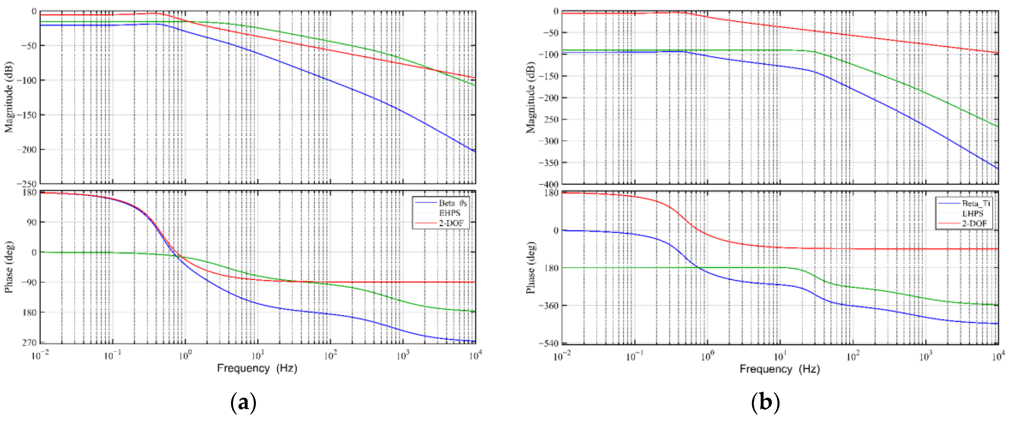
2.1.4. Steering System Characteristic Analysis

In order to analyze the characteristics of the EHPS system, the mechanical and hydraulic dynamic should be fully derived. Regardless of the friction of the steering column, the mechanical system is linear, but the hydraulic system is nonlinear due to the hydraulic assistance. Equations (1) and (2) can be rephrased as follows.

$$J_s{\ddot{\theta }}_s+B_s{\dot{\theta }}_s+K_t{\theta }_s-K_t{R}_t{r}_{cs}{\theta }_f=T_i$$

(8)

$$M_p{r}_{cs}{\ddot{\theta }}_f+B_p{r}_{cs}{\dot{\theta }}_f+\left(K_r+K_t{R_t}^2{r}_{cs}\right){\theta }_f=K_t{R}_t{\theta }_{\omega }+K_{\mathsf{\Psi }}·\mathsf{\Psi }\left(T_t\right)$$

(9)

Take the Laplace transform of Equations (8) and (9) and get the following:

$$J_s{s}^2{\theta }_s\left(s\right)+B_{s}s{\theta }_s\left(s\right)+K_t{\theta }_s\left(s\right)-K_t{R}_t{r}_{cs}{\theta }_f\left(s\right)=T_i\left(s\right)$$

(10)

$$M_p{r}_{cs}{s}^2{\theta }_f\left(s\right)+B_p{r}_{cs}s{\theta }_f\left(s\right)+\left(K_r+K_t{R_t}^2{r}_{cs}\right){\theta }_f\left(s\right)=K_t{R}_t{\theta }_s\left(s\right)+K_{\mathsf{\Psi }}·\mathsf{\Psi }\left(T_t\right)$$

(11)

where ${\theta }_s\left(s\right)$, ${\theta }_f\left(s\right)$ are the Laplace transforms of ${\theta }_s$, ${\theta }_f$; $T_i\left(s\right)$ is the Laplace transform of $T_i$.

The transfer function of EHPS from the front wheel to the steering wheel can be described as:

$$\frac{{\theta }_f\left(s\right)}{{\theta }_s\left(s\right)}=\frac{A_p·K_t·K_A+R_t·K_t}{M_n{s}^2+\left(B_n-K_q·A_p\right)s+\left[K_f+R_t·K_t\left(R_t+K_A\right)\right]}·\frac{1}{r}$$

(12)

The transfer function of EHPS from front wheel to steering torque can be described as:

$$\frac{{\theta }_f\left(s\right)}{T_i\left(s\right)}=\frac{{\theta }_f\left(s\right)}{{(J_s{s}^2+B_{s}s+K_t)\theta }_s\left(s\right)-K_t·K_t·r}$$

(13)

Take the parameter values in

Table 1. The parameters used in the EHPS system dynamic model.

Parameters	Values	Parameters	Values
$J_s$/(kg·m2)	0.0258	$R_t$	459
$B_s$/(Nm·s/rad)	0.742	$M_p$/kg	8.07
$K_t$/(Nm/rad)	143.2	$B_p$/(Nm/s)	35,283
$r_{cs}$/m	0.05	$K_R$/(Nm/rad)	5730
$C_d$	0.5	$\rho$/($\mathrm{k}\mathrm{g}/{\mathrm{m}}^3$)	880
$\beta$/($\mathrm{N}/{\mathrm{m}}^2$)	1.4 × 105	$A_p$/(${\mathrm{m}}^2$)	9.4 × 10−3

and set ${\theta }_f=\delta$, the Equations (12) and (13) can be expressed as:

$$\frac{\delta \left(s\right)}{{\theta }_s\left(s\right)}=\frac{7020}{0.4035s^2+1764s+40010}$$

(14)

$$\frac{\delta \left(s\right)}{T_i\left(s\right)}=\frac{7020}{0.0112s^4+45.83s^3+2404s^2+282287s-2.25e8}$$

(15)

2.2. Dynamic Models of 2-DOF Vehicle

The 2-DOF vehicle model can reflect the lateral characteristics of the vehicle accurately with a small calculated load and is often utilized to analyze the relationship between the yaw rate and the sideslip angle when the vehicle is moving on a plane. The 2-DOF model describing vehicle motion is based on the following idealized assumptions:

• Vehicle driving on a flat road, no vertical road uneven input;
• Ignore the steering transmission system and apply the input directly to the wheel;
• Longitudinal velocity as a constant, and ignore the effect of aerodynamics;
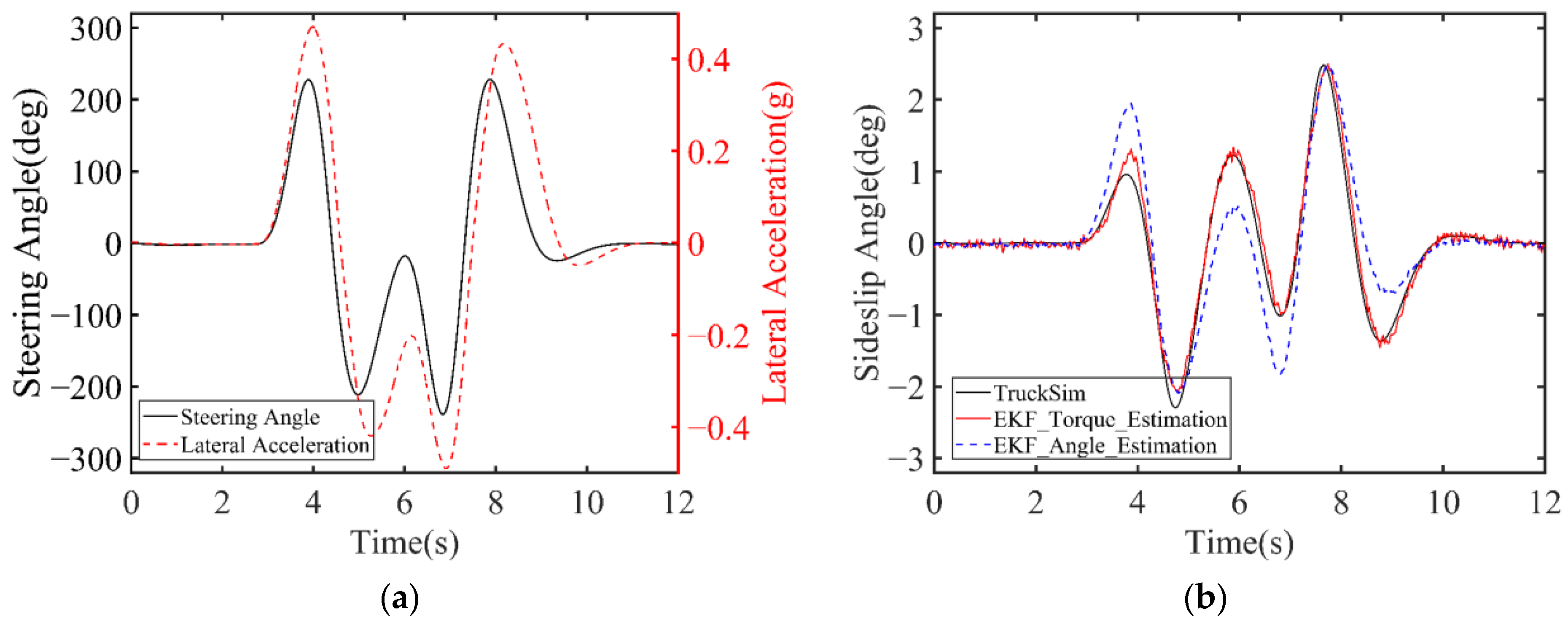
• The lateral acceleration is limited to less than 0.4 g, and the tire cornering characteristics are in a linear range.

Therefore, the car is simplified into a two-wheeled bicycle model, as shown in Figure 3, and its dynamic model is represented as:

$$\left\{\begin{array}{l}m{a}_y=F_{yf}+F_{yr}\\ { I}_z\dot{\gamma }=F_{yf}{l}_f-F_{yr}{l}_r\end{array}\right.$$

(16)

where $m$ is the mass of the vehicle; $a_y$ is the lateral acceleration; $F_{yf}$ and $F_{yr}$ are the lateral tire forces; ${ I}_z$ is yaw moment of inertia;$\dot{ \gamma }$ the yaw acceleration the yaw acceleration; $l_f$ and $l_r$ are the distance from the vehicle’s center of mass to the front and rear axles. By using the kinematic formula, we can rewrite ${{ a}_y,F}_{yf}{,F}_{yr}$ in terms of $u,v, \beta ,\gamma$.

$$a_y=v+u\gamma , \beta =\frac{u}{v},F_{yf}=k_1{\alpha }_f,F_{yr}=k_2{\alpha }_r, {\alpha }_f=\beta +\frac{l_f\gamma }{u}-\delta ,{\alpha }_r=\beta -\frac{l_r\gamma }{u}$$

(17)

The linear 2-DOF vehicle model can be obtained by arranging Equations (16) and (17). This lays the foundation for analyzing the impact of the steering wheel angle and torque on the vehicle’s sideslip angle.

$$\left\{\begin{array}{l}mu\left(\dot{\beta }+\gamma \right)=\left(k_1+k_2\right)\beta +\frac{l_f{k}_1-l_r{k}_1}{u}\gamma -k_1\delta \\ { I}_z\dot{\gamma }=\left(k_1+k_2\right)\beta +\frac{{l_f}^2{k}_1+{l_r}^2{k}_1}{u}\gamma -l_f{k}_1\delta \end{array}\right.$$

(18)

2.3. Transfer Function Analysis of Vehicle Dynamics Model

The transfer function is an important tool for modeling, analysis, and design of control systems. By establishing the transfer function between the steering wheel angle, torque, and 2-DOF vehicle model, the characteristics of the center of sideslip angle during vehicle steering can be further analyzed.

The Laplace transform of Formula (18) is as follows:

$$\left\{\begin{array}{l}mu\left[s·\beta \left(s\right)+\gamma (s)\right]=\left(k_1+k_2\right)\beta (s)+\frac{l_f{k}_1-l_r{k}_1}{u}\gamma \left(s\right)-k_1\delta \left(s\right)\\ { I}_{z}s\gamma (s)=\left(k_1+k_2\right)\beta (s)+\frac{{l_f}^2{k}_1+{l_r}^2{k}_1}{u}\gamma (s)-l_f{k}_1\delta (s)\end{array}\right.$$

(19)

After simplification, the transfer function between the sideslip angle and the front wheel angle can be obtained, where the input signal is the front wheel angle and the output signal is the sideslip angle, as shown in Equation (18).

$$G_{\beta \delta }\left(s\right)=\frac{\beta \left(s\right)}{\delta \left(s\right)}=\frac{Y\left(s\right)}{X\left(s\right)}=\frac{5.64{\times 10}^{9}s-2.74\times {10}^{10}}{6.20\times {10}^9{s}^2+1.80\times {10}^{10}s+5.22{\times 10}^{10}}$$

(20)

where

$$\left\{\begin{array}{l}X\left(s\right)={ muI}_z{s}^2-\left[\left(k_1+k_2\right){ I}_z+muM\right]s+\left(k_1+k_2\right)M+({l_{f}k}_1-{l_{r}k}_2)(mu-N)\\ Y\left(s\right)=-k_1{ I}_{z}s+k_{1}M+l_f{k}_1(mu-N)\\ M=\frac{{{l_f}^{2}k}_1+{{l_r}^{2}k}_2}{u}\\ N=\frac{{l_{f}k}_1-{l_{r}k}_2}{u}\end{array}\right.$$

(21)

By solving Equations (12), (13) and (20), we can obtain the transfer function between steering wheel angle and sideslip angle, as well as the transfer function relationship between steering wheel torque and sideslip angle.

$$G_1\left(s\right)=\frac{\beta \left(s\right)}{{\theta }_s\left(s\right)}=\frac{\beta \left(s\right)}{\delta \left(s\right)}\frac{\delta \left(s\right)}{{\theta }_s\left(s\right)}=\frac{3.96\times {10}^{13}s-1.92{\times 10}^{14}}{2.50{\times 10}^9{s}^4+1.10\times {10}^{13}{s}^3+2.80{\times 10}^{14}{s}^2+8.10{\times 10}^{14}s+2.09\times {10}^{15}}$$

(22)

$$G_2\left(s\right)=\frac{\beta \left(s\right)}{T_i\left(s\right)}=\frac{\beta \left(s\right)}{T_i\left(s\right)}\frac{T_i\left(s\right)}{{\theta }_s\left(s\right)}=\frac{3.96\times {10}^{13}s-1.92{\times 10}^{14}}{\begin{array}{c}(6.95{\times 10}^7{s}^6+2.84\times {10}^{11}{s}^5+1.57{\times 10}^{13}{s}^4+1.80\times {10}^{15}{s}^3\\ -1.39\times {10}^{18}{s}^2-4.02{\times 10}^{18}s-1.18{\times 10}^{19})\end{array}}$$

(23)

Through the previous derivation, we obtained the transfer function between the steering wheel angle, steering wheel torque, and the sideslip. The frequency analysis of the transfer function can obtain the corresponding amplitude and frequency characteristics in Figure 4.

In Figure 4, it can be seen that when the frequency of the steering system is in the range of ${10}^{-2}$ to ${10}^{-1}$ Hz, the phase in Figure 4a has a phase advance of ${180}^{°}$, while there is a small phase lag in Figure 4b, which ranges from 0 to −${19}^{°}$. In the frequency range of ${10}^{-1}$~${10}^0$ Hz, there is a significant decrease in the phase of both plots, from ${158}^{°}$ advance to ${38}^{°}$ lag (${158~-38}^{°}$) in Figure 4a, while from ${19}^{°}$ lag to ${200}^{°}$ lag (${-19~-200}^{°}$) in Figure 4b. It can be seen that the phase difference in Figure 4a is larger than in Figure 4b, which is ${196}^{°}$ and ${181}^{°}$, respectively. Moreover, it can be seen from the amplitude characteristics that the amplitude of Figure 4a is greater than that of Figure 4b, indicating that the amplitude ratio of Figure 4a is greater than that of Figure 4b, which is −20.4 dB and −95.4 dB, respectively.

According to Equations (22) and (23), the transfer function of the sideslip angle includes the steering angle, steering torque, and front-wheel angle parameters. In order to further explore its characteristics, the transfer function is decomposed into transfer functions based on the EHPS model and 2-DOF model for analysis. The Bode diagram results of the transfer function are shown in Figure 5.

It can be seen from Figure 5 that in the range of ${10}^{-2}$ to ${ 10}^0$ Hz, the 2-DOF model of the vehicle will produce a large phase overshoot, with the phase changing from ${178}^{°}$ to $-{22}^{°}$, which is the main source of phase overshoot of the system. The EHPS transfer function based on the steering angle in Figure 5a has a phase lag of almost 0 in the range of ${10}^{-2}$ to ${ 10}^0$ Hz, while the torque-based transfer function in Figure 5b has a phase lag of 180°. The EHPS model transfer function based on steering torque can rectify phase lead better than the transfer function based on steering angle. Therefore, the estimation of sideslip angle based on steering torque can more accurately reflect the real status of the vehicle.

3. Design of EKF State Observer

The Kalman filter algorithm has a good effect on the state estimation of linear systems, but the actual system often has different degrees of nonlinearity, so it cannot achieve the optimal estimation effect when dealing with problems in nonlinear scenarios. For the state estimation problem of a nonlinear system, the EKF algorithm is generally used. The nonlinear system is expanded by Taylor at the best estimation point, only the first-order system part is retained for linearization, and then the recursive operation is realized by using the classical KF formula.

In this section, a sideslip angle estimation method is proposed, which is based on steering torque instead of steering angle. The 2-DOF model and EHPS model are used for observer design, and the nonlinear state space equation is expressed as follows:

$$\left\{\begin{array}{l} \dot{x}\left(t\right)=f\left(x\left(t\right),u\left(t\right)\right)+\omega \left(t\right)\\ y\left(t\right)=h\left(x\left(t\right)\right)+v\left(t\right)\end{array}\right.$$

(24)

where $\mathit{x}$ is the state vector, $\mathit{x}={[{\dot{\theta }}_s {\theta }_s \dot{\delta } \delta \gamma \beta ]}^T$; $\mathit{u}$ is the control vector, $\mathit{u}=\delta$; $\mathit{y}$ is the measurement output, $\mathit{y}={[{\dot{\theta }}_s {\theta }_s \dot{\delta } \delta a_y \gamma ]}^T$; $\mathit{\omega }$ and $\mathit{v}$ are the Gaussian white noise; $\mathit{Q}$ and $\mathit{R}$ are defined as the system noise $\mathit{\omega }$ covariance matrix and the measurement noise $\mathit{v}$ covariance matrix, respectively.

According to Equations (1)–(12) of the EHPS model and 2-DOF model, the state equations and measurement equations can be expressed as follows.

State equations:

$$\left\{\begin{array}{l}{\ddot{\theta }}_s=\frac{1}{J_s}{T}_i-\frac{B_s}{J_s}{\dot{\theta }}_s-\frac{K_t}{J_s}{\theta }_s+\frac{K_t·x_p}{J_s·r}\\ {\dot{\theta }}_s={\dot{\theta }}_s\\ \ddot{\delta }=\frac{[A_p{p}_l\left(q\right)+R_t]K_t}{M_n}{\theta }_s-\frac{B_n}{M_n}\dot{\delta }-\frac{\left[K_f+K_t{R}_t\left(A_p{p}_l\left(q\right)+R_t\right)\right]r}{M_n}\delta \\ \dot{\delta }=\dot{\delta }\\ \dot{\gamma }=\frac{l_f{F}_{yf}-l_r{F}_{yr}}{I_z}\\ \dot{\beta }=\frac{F_{yf}+F_{yr}}{mu}-\gamma \end{array}\right.$$

(25)

Measurement equations:

$$\left\{\begin{array}{l}{\dot{\theta }}_s={\dot{\theta }}_s\\ {\theta }_s={\theta }_s\\ \dot{\delta }=\dot{\delta }\\ \delta =\delta \\ a_y=\frac{F_{yf}+F_{yr}}{m}-\gamma \\ \gamma =\gamma \end{array}\right.$$

(26)

where $F_{yf}$ and $F_{yr}$ can be obtained from the magic formula model, which can be expressed as follows:

$$\left\{\begin{array}{l}{F}_{yf}=D_f\sin \left(C_f\arctan \right(B_f{\alpha }_f-E_f(B_f{\alpha }_f-\arctan (B_f{\alpha }_f\left)\right)\left)\right)\\ F_{yr}=D_r\sin \left(C_r\arctan \right(B_r{\alpha }_r-E_r(B_r{\alpha }_r-\arctan (B_r{\alpha }_r\left)\right)\left)\right)\end{array}\right.$$

(27)

where $B_f$~$E_f$ are the front wheel side force coefficient, and $B_r$~$E_r$ are the rear wheel side force coefficient, which can be obtained in

Table 2. The parameters used in the magic formula (MF) model.

${\mathit{B}}_{\mathit{f}}$	${\mathit{C}}_{\mathit{f}}$	${\mathit{D}}_{\mathit{f}}$	${\mathit{E}}_{\mathit{f}}$	${\mathit{B}}_{\mathit{r}}$	${\mathit{C}}_{\mathit{r}}$	${\mathit{D}}_{\mathit{r}}$	${\mathit{E}}_{\mathit{r}}$
0.12	1.6	2.35 × 104	−0.3028	0.012	1.6	12,710	−0.3028

.

By obtaining the Jacobian matrix from the state equations and the measurement equations and linearizing the model, the following expressions can be obtained.

$$F\left(t\right)=\left[\begin{array}{cccccc}-\frac{B_s}{J_s}& -\frac{B_s}{J_s}{\ddot{\theta }}_s& 0& 0& 0& 0\\ 1& {\ddot{\theta }}_s& 0& 0& 0& 0\\ 0& \frac{[A_p{p}_l(q)+R_t]K_t}{M_n}& \frac{B_n}{M_n}& \frac{B_n}{M_n}\ddot{\delta }+\frac{[K_f+K_t{R}_t(A_p{p}_l(q)+R_t)]r}{M_n}& 0& 0\\ 0& 0& 1& \ddot{\delta }& 0& 0\\ 0& 0& 0& 0& 0& 0\\ 0& 0& 0& 0& -1& 0\end{array}\right]$$

(28)

$$H\left(t\right)=\left[\begin{array}{cccccc}1& {\ddot{\theta }}_s& 0& 0& 0& 0\\ 0& 1& 0& 0& 0& 0\\ 0& 0& 1& \ddot{\delta }& 0& 0\\ 0& 0& 0& 1& 0& 0\\ 0& 0& 0& 0& -1& 0\\ 0& 0& 0& 0& 1& 0\end{array}\right]$$

(29)

The nonlinear state space Equation (24) is discretized by the Euler approximation method, and the following expression can be obtained.

$$\left\{\begin{array}{l}{x}_k=f\left(x_{k-1},u_{k-1}\right)+{\omega }_{k-1}\\ y_k=h\left(x_k\right)+v_k\end{array}\right.$$

(30)

The recursive algorithm of EKF is described as follows:

• Time update

The state estimate time update

$${{\widehat{x}}_k}^{-}=f\left({\widehat{x}}_{k-1},u_{k-1}\right)$$

(31)

The error covariance time update

$${P_k}^{-}=A_k{P}_{k-1}{A_k}^T+\mathrm{Q}$$

(32)

where $A_k$ is the process Jacobin matrix, which is the partial derivative of $f\left({\widehat{x}}_{k-1},u_{k-1}\right)$ to the state vector $\mathit{x}$, and it can be expressed as

$$A_k=\frac{\partial f\left(x_{k-1},u_{k-1}\right)}{\partial x}$$

(33)

2.

Measurement update

$$K_k=\frac{{P_k}^{-}{H_k}^T}{H_k{P_k}^{-}{H_k}^T+R}$$

(34)

$${\widehat{x}}_k={{\widehat{x}}_k}^{-}+K_k[y_k-h\left({{\widehat{x}}_k}^{-}\right)]$$

(35)

$$P_k={P_k}^{-}-K_k{H}_k{P_k}^{-}$$

(36)

where $H_k$ is the measurement Jacobin matrix, which is the partial derivative of $h\left(x_k\right)$ to the state vector $\mathit{x}$, and it can be expressed as

$$H_k=\frac{\partial h\left(x_k\right)}{\partial x}$$

(37)

4. Results and Discussion

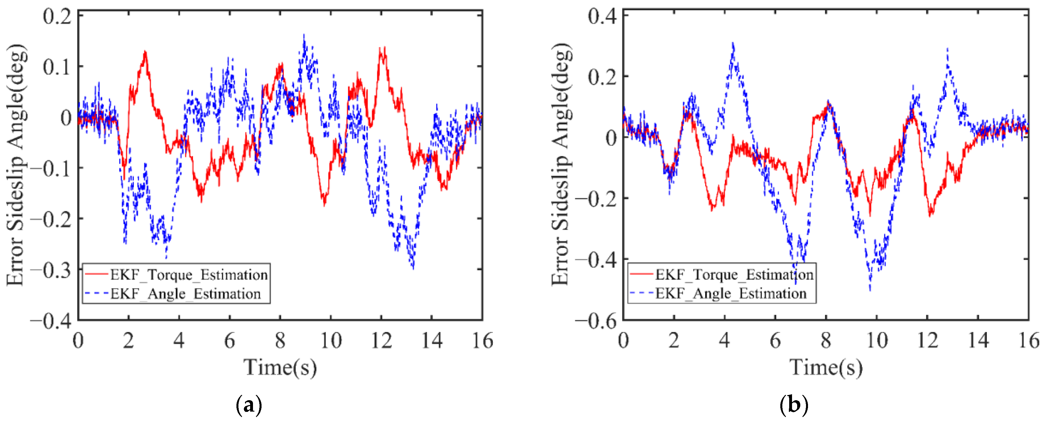
4.1. Simulation Results

The proposed estimation method is tested based on TruckSim and Matlab/Simulink environment, which can simulate the driving conditions of the vehicle in the real environment and provide all the data needed for the vehicle model. The vehicle parameters required in the EKF algorithm simulation are shown in

Table 3. The parameters used in TruckSim.

Parameters	Symbols	Values
Sprung mass	$m_s$	4455 (kg)
Front axle unsprung mass	$m_f$	607.3 (kg)
Rear axle unsprung mass	$m_r$	1144 (kg)
Distance between the front axle and the vehicle gravity center	$l_f$	1.25 (m)
Distance between the rear axle and the vehicle gravity center	$l_r$	3.75 (m)
Yaw moment inertia of the whole vehicle	$I_z$	34,802.6 ($\mathrm{k}\mathrm{g}·{\mathrm{m}}^2$)
Front cornering stiffness	$k_1$	$1.31 \times {10}^4(\mathrm{N}/\mathrm{r}\mathrm{a}\mathrm{d}$)
Rear cornering stiffness	$k_2$	$5.11 \times {10}^3(\mathrm{N}/\mathrm{r}\mathrm{a}\mathrm{d}$)

, which are available in TruckSim.

The simulation results are shown in Figure 6, Figure 7 and Figure 8. The simulation tests have been conducted at the adhesion coefficient of 0.85 and 0.75, which normally show a high-µ value and a low-$\mu$ value, respectively. When the vehicle speed is 50 km/h and the adhesion coefficient is high, the vehicle is considered to be in the linear region (the lateral acceleration is less than 0.4 g). The vehicle is considered to be in a nonlinear region when the speed is 65 km/h and the adhesion coefficient is low (the lateral acceleration is greater than 0.4 g). Figure 6 shows the results carried out on the adhesion coefficient of 0.85 and the vehicle speed at 50 km/h.

Figure 6a shows the driving conditions, including steering wheel angle and lateral acceleration, where the steering angle amplitude is ${90}^{°}$. According to Figure 6b, the proposed sideslip angle observer based on steering torque shows better estimation performance compared with the results based on steering angle, which is generally consistent with the properties analyzed in Section 2.3. As can be seen from the double line change driving condition in Figure 7, when the adhesion coefficient increases, the estimation of sideslip angle based on torque is more consistent with the TruckSim output results, while the estimation based on steering angle has obvious phase advance. From Figure 8, we can see that when the steering angle reaches ${300}^{°}$, the vehicle is put under a critical driving condition and is generally considered to be in a nonlinear region (the lateral acceleration is 0.46 g). According to Figure 8b, in the nonlinear region, the accuracy of sideslip estimation based on steering torque is better than that based on steering angle.

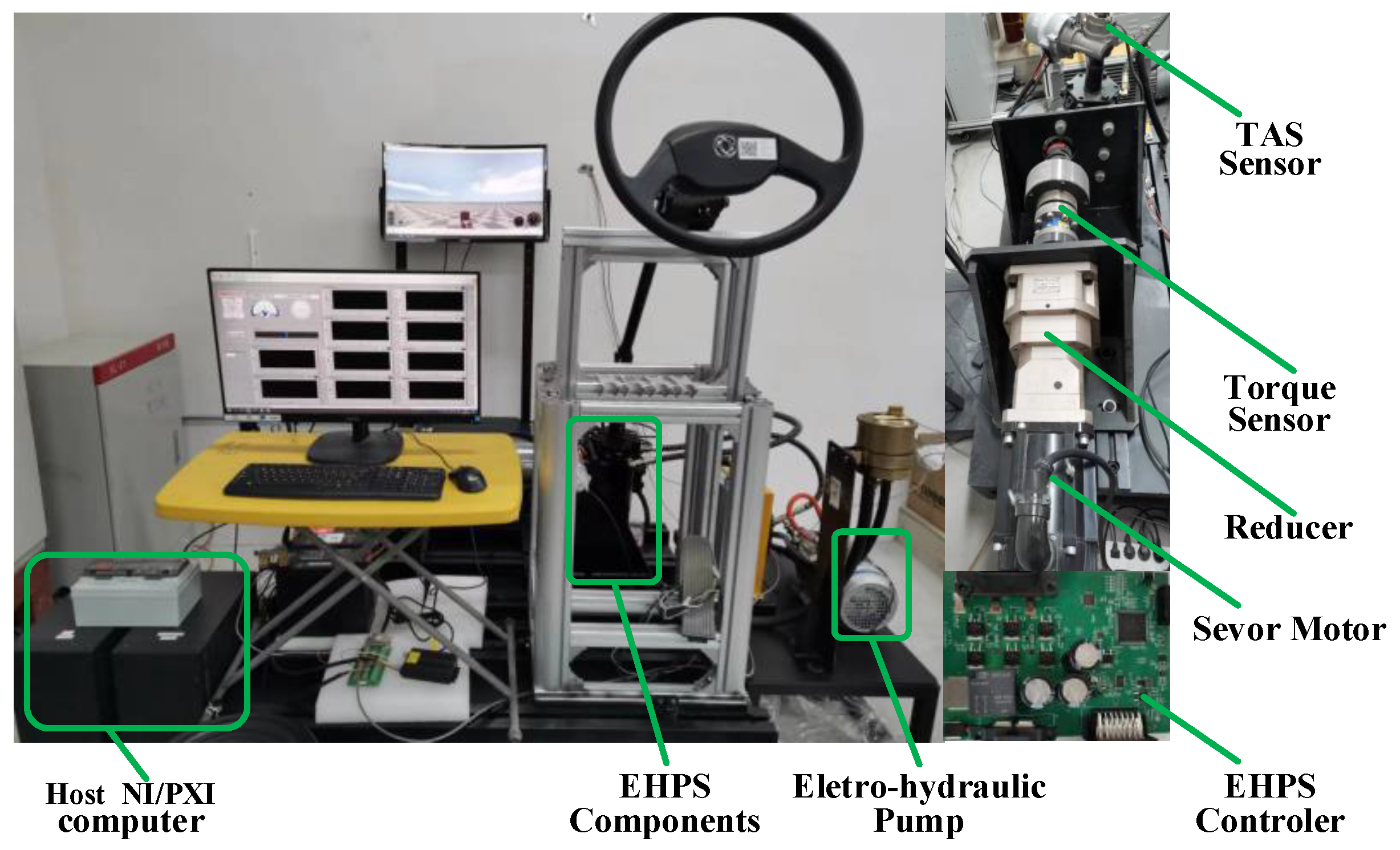
4.2. Test Bench Results

In order to verify the effectiveness of the proposed method, a hardware-in-the-loop (HIL) test bench is built, as shown in Figure 9. The test bench mainly consists of an electric–hydraulic power steering system (EHPS), an electro-hydraulic pump, a servo motor and reducer to provide steering resistance, a torque angle sensor, a control unit based on MPC5741, a host computer, and an NI/PXI real-time system to provide vehicle running environment. The signal between the EHPS controller unit and the host computer communicates through a CAN module. The sideslip angle estimation algorithm proposed in this paper is recorded into the controller for calculation, and the real sideslip angle is output through TruckSim. The estimated results and real results are obtained through the CAN bus.

Hardware-in-the-loop test conditions adopt double line change conditions, which is a common working condition when the vehicle changes lanes. The vehicle speed is 50 km/h, and the road adhesion coefficient is 0.85; the test results are shown in Figure 10.

From Figure 10a, we can see that the maximum value of lateral acceleration is 0.37 g when the time is 13 s. Here, we can assume that the vehicle is driving in the linear region. It can be seen from Figure 10b that the sideslip angle based on the steering angle estimation is slightly ahead in phase and overshoots in amplitude. However, the sideslip angle based on the torque estimation is more accurately matched to the real value.

Figure 11 shows the estimated and measured sideslip angle under the condition that the vehicle speed is 65 km/h and the adhesion coefficient is 0.75. As shown in Figure 11a, the lateral acceleration reaches −0.4 g at 6.4 s and exceeds 0.5 g at 12 s. In general, we can assume that the vehicle has reached the nonlinear instability stage. Based on Figure 11b, we can see that the estimated sideslip angle based on the steering torque matches the real value more accurately than the ones based on the steering angle. Figure 12a shows the error between the two methods of sideslip angle estimation and the real angle. The maximum error of the sideslip angle based on the steering angle estimation and the steering torque estimation is 0.17° and 0.3°, respectively. The average error values of the two estimation methods are 0.06° and 0.08°, respectively. From Figure 12b, it can be seen that the error amplitude based on steering torque estimation is smaller than that based on steering angle estimation, and the average error values are 0.08° and 0.12°, respectively.

The mean absolute error (MSE) and root mean square error (RSME) results based on steering angle and steering torque methods are shown in

Table 4. The estimation error in different test conditions.

Maneuver	Method	Max Error (°)	MAE (°)	RMSE (°)
Double line change u = 50 km/h µ = 0.85	Steering torque estimation	−0.175	0.0613	0.0733
	Steering angle estimation	−0.3	0.0805	0.1112
Double line change u = 65 km/h µ = 0.75	Steering torque estimation	−0.26	0.0822	0.1032
	Steering angle estimation	−0.51	0.1257	0.1739

. From Table 4, we can know that the maximum error value of the estimated sideslip angle based on steering torque is smaller than that based on the steering angle, whether on high- or low-adhesion roads. Under high-adhesion road conditions, the MSE indexes of estimated sideslip angle based on steering torque and steering angle are 0.0613 and 0.0805, and the estimation accuracy is improved by 23.9%. In addition, under low-adhesion road conditions, the MSE indexes of estimated sideslip angle based on steering torque and steering angle are 0.0822 and 0.1257, and the estimation accuracy is improved by 34.6%.

5. Conclusions

The sideslip angle estimation of intelligent commercial vehicles based on steering torque using the EKF algorithm is proposed in this paper. First, the transfer functions between the sideslip angle–torque and sideslip angle–angle are constructed. Then, based on the analysis of transfer functions, it is found that the steering torque signal has an accurate and more direct response due to the hydraulic pressure in the EHPS system. To estimate the vehicle sideslip angle, a state observer derived from the extended Kalman filter (EKF) method is proposed. Both simulation and test bench results show that the sideslip angle estimated based on steering torque has a smaller phase lead and higher accuracy than the sideslip angle estimated based on steering angle in the linear region and nonlinear region. The experimental results show that the accuracy of estimation sideslip angle based on steering torque is improved by 23.9% and 34.6% compared with that based on steering angle under high-adhesion road conditions and low-adhesion road conditions, respectively. However, the proposed method is applied to a bench test in this paper, so its application for a real car test will be studied in the future. In addition, side angle estimation will be very important for autonomous vehicles and connected automated vehicles. It is also interesting to use the automated driving systems data acquisition and analytics platform technology and 3D lidar fusion sensing technology to enhance the performance of side angle estimation.

References

1. Cheng, S.; Li, L.; Chen, J. Fusion Algorithm Design Based on Adaptive SCKF and Integral Correction for Side-Slip Angle Observation. IEEE Trans. Ind. Electron. 2018, 65, 5754–5763. [Google Scholar] [CrossRef]
2. Zhao, B.; Xu, N.; Chen, H.; Guo, K.; Huang, J. Stability control of electric vehicles with in-wheel motors by considering tire slip energy. Mech. Syst. Signal Process. 2019, 118, 340–359. [Google Scholar] [CrossRef]
3. Xia, X.; Xiong, L.; Lu, Y.; Gao, L.; Yu, Z. Vehicle sideslip angle estimation by fusing inertial measurement unit and global navigation satellite system with heading alignment. Mech. Syst. Signal Process. 2021, 150, 107290. [Google Scholar] [CrossRef]
4. Wang, Y.; Geng, K.; Xu, L.; Ren, Y.; Dong, H.; Yin, G. Estimation of Sideslip Angle and Tire Cornering Stiffness Using Fuzzy Adaptive Robust Cubature Kalman Filter. IEEE Trans. Syst. Man Cybern. Syst. 2022, 52, 1451–1462. [Google Scholar] [CrossRef]
5. Tin Leung, K.; Whidborne, J.F.; Purdy, D.; Dunoyer, A. A review of ground vehicle dynamic state estimations utilising GPS/INS. Veh. Syst. Dyn. 2011, 49, 29–58. [Google Scholar] [CrossRef]
6. Anderson, R.; Bevly, D.M. Using GPS with a model-based estimator to estimate critical vehicle states. Veh. Syst. Dyn. 2010, 48, 1413–1438. [Google Scholar] [CrossRef]
7. Cheng, S.; Wang, Z.; Yang, B.; Nakano, K. Convolutional Neural Network-Based Lane-Change Strategy via Motion Image Representation for Automated and Connected Vehicles. IEEE Trans. Neural Netw. Learn. Syst. 2023, 1–12. [Google Scholar] [CrossRef]
8. Liu, W.; Xiong, L.; Xia, X.; Lu, Y.; Gao, L.; Song, S. Vision-aided intelligent vehicle sideslip angle estimation based on a dynamic model. IET Intell. Transp. Syst. 2020, 14, 1183–1189. [Google Scholar] [CrossRef]
9. Kanghyun, N.; Fujimoto, H.; Hori, Y. Lateral Stability Control of In-Wheel-Motor-Driven Electric Vehicles Based on Sideslip Angle Estimation Using Lateral Tire Force Sensors. IEEE Trans. Veh. Technol. 2012, 61, 1972–1985. [Google Scholar] [CrossRef]
10. Guo, J.; Luo, Y.; Li, K.; Dai, Y. Coordinated path-following and direct yaw-moment control of autonomous electric vehicles with sideslip angle estimation. Mech. Syst. Signal Process. 2018, 105, 183–199. [Google Scholar] [CrossRef]
11. Wang, Z.; Qin, Y.; Gu, L.; Dong, M. Vehicle System State Estimation Based on Adaptive Unscented Kalman Filtering Combing with Road Classification. IEEE Access 2017, 5, 27786–27799. [Google Scholar] [CrossRef]
12. Cheng, C.; Cebon, D. Parameter and state estimation for articulated heavy vehicles. Veh. Syst. Dyn. 2011, 49, 399–418. [Google Scholar] [CrossRef]
13. Gadola, M.; Chindamo, D.; Romano, M.; Padula, F. Development and validation of a Kalman filter-based model for vehicle slip angle estimation. Veh. Syst. Dyn. 2013, 52, 68–84. [Google Scholar] [CrossRef] [Green Version]
14. Piyabongkarn, D.; Rajamani, R.; Grogg, J.A.; Lew, J.Y. Development and Experimental Evaluation of a Slip Angle Estimator for Vehicle Stability Control. IEEE Trans. Control Syst. Technol. 2009, 17, 78–88. [Google Scholar] [CrossRef]
15. Leung, K.T.; Whidborne, J.F.; Purdy, D.; Barber, P. Road vehicle state estimation using low-cost GPS/INS. Mech. Syst. Signal Process. 2011, 25, 1988–2004. [Google Scholar] [CrossRef] [Green Version]
16. Wu, Z.; Yao, M.; Ma, H.; Jia, W. Improving Accuracy of the Vehicle Attitude Estimation for Low-Cost INS/GPS Integration Aided by the GPS-Measured Course Angle. IEEE Trans. Intell. Transp. Syst. 2013, 14, 553–564. [Google Scholar] [CrossRef]
17. Yoon, J.-H.; Peng, H. A Cost-Effective Sideslip Estimation Method Using Velocity Measurements from Two GPS Receivers. IEEE Trans. Veh. Technol. 2014, 63, 2589–2599. [Google Scholar] [CrossRef]
18. Xiong, L.; Xia, X.; Lu, Y.; Liu, W.; Gao, L.; Song, S.; Yu, Z. IMU-Based Automated Vehicle Body Sideslip Angle and Attitude Estimation Aided by GNSS Using Parallel Adaptive Kalman Filters. IEEE Trans. Veh. Technol. 2020, 69, 10668–10680. [Google Scholar] [CrossRef]
19. Xia, X.; Hashemi, E.; Xiong, L.; Khajepour, A. Autonomous Vehicle Kinematics and Dynamics Synthesis for Sideslip Angle Estimation Based on Consensus Kalman Filter. IEEE Trans. Control Syst. Technol. 2023, 31, 179–192. [Google Scholar] [CrossRef]
20. Huang, S.; Cao, W.; Qian, R.; Liu, Y.; Ji, X. Front wheel angle tracking control research of intelligent heavy vehicle steering system. Proc. Inst. Mech. Eng. Part C J. Mech. Eng. Sci. 2020, 235, 3454–3467. [Google Scholar] [CrossRef]
21. Wu, J.; Zhao, Y.; Ji, X.; Liu, Y.; Zhang, L. Generalized internal model robust control for active front steering intervention. Chin. J. Mech. Eng. 2015, 28, 285–293. [Google Scholar] [CrossRef]
Figure 1. Schematic diagram of the EHPS system.
Applsci 13 07974 g001
Figure 2. Schematic diagram of the mechanical system.
Applsci 13 07974 g002
Figure 3. Schematic diagram of the 2-DOF vehicle model.
Applsci 13 07974 g003
Figure 4. The Bode diagrams of two methods: (a) The Bode diagram of steering angle and sideslip angle; (b) The Bode diagram of steering torque and sideslip angle.
Applsci 13 07974 g004
Figure 5. The resolved Bode diagrams of two methods: (a) The Bode diagram of steering wheel angle and sideslip angle; (b) The Bode diagram of steering wheel torque and sideslip angle.
Applsci 13 07974 g005
Figure 6. The simulation results at u = 50 km/h, μ = 0.75: (a) Driving condition and lateral acceleration; (b) The estimation result of sideslip angle with 90°, 1 Hz.
Applsci 13 07974 g006
Figure 7. The simulation results at u = 50 km/h, μ  = 0.85: (a) Driving condition and lateral acceleration; (b) The estimation result of sideslip angle with double line change.
Applsci 13 07974 g007
Figure 8. The simulation results at u = 65 km/h, μ = 0.75: (a) Driving condition and lateral acceleration; (b) The estimation result of sideslip angle with double line change.
Applsci 13 07974 g008
Figure 9. Structure of hardware-in-the-loop test bench.
Applsci 13 07974 g009
Figure 10. The test bench results at u = 50 km/h, μ = 0.85: (a) Driving condition and lateral acceleration; (b) The estimation result of sideslip angle with double line change.
Applsci 13 07974 g010
Figure 11. The test bench results at u = 65 km/h, μ = 0.75: (a) Driving condition and lateral acceleration; (b) The estimation result of sideslip angle with double line change.
Applsci 13 07974 g011
Figure 12. The errors of sideslip angle between two methods: (a) The results at u = 50 km/h, μ = 0.85; (b) The results at u = 65 km/h, μ   = 0.75.
Applsci 13 07974 g012