Modified Maximum Likelihood Estimation Metal Magnetic Memory Quantitative Identifying Model of Weld Defect Levels Based on Dempster–Shafer Theory

Abstract

Metal magnetic memory (MMM) is a nondestructive testing technology based on the magnetomechanical effect, which is widely used in the qualitative detection of stress concentration zones for welded joints. However, there is inevitable residual stress after welding, which brings the bottleneck of quantitative identification between the weld residual stress concentration and the early hidden damage. In order to overcome the bottleneck of quantitative identification of weld defect levels with MMM technology, a modified maximum likelihood estimation (MLE) MMM quantitative identifying model is first proposed. The experimental materials are Q235B welded plate specimens. Fatigue tension experiments were operated to find the MMM feature laws of critical hidden crack by comparing with synchronous X-ray detection results. Six MMM characteristic parameters, which are, ΔH_p(x), G_x^max, Z_x^max, ΔH_p(y), G_y^max and Z_y^max, are extracted corresponding to the normal state, the hidden crack state and the macroscopic crack, respectively. The MLE values of the six parameters are obtained by the kernel density functions with optimized bandwidth from the view of mathematical statistics. Furthermore, the modified MLE MMM quantitative identifying model is established based on D–S theory to overcome the partial overlap of MLE values among different defect levels, of which the uncertainty is as low as 0.3%. The verification result from scanning electron microscopy (SEM) is consistent with the prediction of the modified MLE MMM model, which provides a new method for quantitative identification of weld defect levels.

1. Introduction

Welded joints always work in high temperature, high pressure and corrosive environments, which are prone to cause cracks, fractures and explosions after long-time operation [1]. For this reason, the testing and evaluation of welded joints are very important for pressure vessels, piping and other equipment in service. Principally, it is necessary to identify the early critical state of hidden cracks because accidents caused by hidden cracks may occur at any time [2]. However, the stress concentration zones (SCZs) and early hidden cracks can not be found by traditional nondestructive testing (NDT), such as ultrasonic testing, X-ray inspect and eddy current testing, until the macroscopic crack has been formed [3,4]. A new NDT technology, called metal magnetic memory (MMM) testing, can not only detect macroscopic cracks but also find SCZs and early hidden cracks without any magnetization devices or special treatment for the tested surface [5,6]. Based on the self-magnetization phenomenon of ferromagnetic materials, the MMM magnetic-field intensity H_p is characterized by the polarity varying along the normal component H_p(y) and maximum value along the tangential component H_p(x) on SCZs [7,8].

The appearance of MMM testing brings a great improvement in SCZs and early defect detection. Doubov et al. demonstrated that the natural magnetization can be applied to inspect structural inhomogeneity and residual stresses which formed during the fabrication of ferromagnetic material by the MMM method [9]. Shi et al., established a magnetomechanical model based on a nonlinear constitutive relation, and analyzed the model using the finite element method quantitatively [10]. Avakian et al. presented a constitutive modelling for ferromagnetic materials under multiaxial multifield loading with different boundary conditions, which can predict magnetization, strain and stress [11]. Ni et al. established a damage model represented by MMM characteristics through fatigue experiments of three point bending and developed a fatigue life prediction method based on the relationship of damage parameter and normalized life [12]. Yao evaluated the contact damage of ferromagnetic materials under nonferromagnetic and ferromagnetic indenters by measuring the signals of the magnetic flux leakage [13]. Xu et al. studied the MMM characteristics of buried defects under different load stages and found the strength of the magnetic field and its gradient decrease with the increasing of the burial depth [14]. Liu proposed the contour plot method to visually analyze the size of defects and established a mathematical model of non-uniform magnetic charge for pipeline leak detection. The peak-to-valley spacing and peak-to-valley values in the contour plot of MFL signal can directly reflect the location and size of defects, and the signal eigenvalues follow the trend of first-order decreasing exponential function, and the first-order derivatives of signal eigenvalues show a trend of first decreasing and then increasing with the decrease of mesh size, and the extreme point of the derivative curve is the best mesh size [15,16]. By comparing with the Standard JB4730-2005 of X-ray detection, the authors set up the MMM reliability model and investigated MMM signal characteristics of SCZs for welded joints [17,18,19].

However, the MMM signals of welded joints often take on fuzzy and uncertainty due to the interruption of welding residual stress [20,21]. This brings the bottleneck of quantitative identification of weld defect levels with MMM technology, especially between the weld residual stress concentration and the early hidden damage. In order to overcome the bottleneck, a modified MLE MMM quantitative identifying model is proposed based on D–S theory from the perspective of mathematical statistics and information fusion. First, the welded specimens made of Q235B steel are tested with MMM method and synchronous X-ray detection for comparison under the fatigue tension loading. Six MMM characteristic parameters are extracted for the normal state, the hidden crack and the macroscopic crack, respectively. Then, the probability density functions of the six MMM characteristic parameters are obtained based on optimized kernel density function, and an MLE MMM model is established for weld defect level identification. Furthermore, the reliability function is established by calculating the proximity of the MLE value of different defect levels considering that in the identification results from the MLE MMM model exist partial overlaps. The D–S decision rules are obtained by allocating and fusing reliability function. Finally, the MLE MMM quantitative identifying model is innovatively presented based on D–S theory. The modified model solves the overlapping and fuzzy problem of different weld defect levels in MMM signal analysis. The proved results show the uncertainty degree is 0.3%, which provides a new idea of MMM quantitative identification of weld defect levels.

2. Experiments

Steel Q235B, widely used in practical engineering, was selected for the base material of welded plate specimens and H08Mn2SiA for the welding wire. The chemical composition and mechanical properties of Steel Q235B are shown in

Table 1. The chemical composition of experimental material (wt.%).

C	Si	Mn	P	S
≤0.20	≤0.35	≤1.40	≤0.045	≤0.045

and

Table 2. The mechanical property of experimental material.

Yield Strength σs/MPa	Ultimate Strength σb/MPa	Percentage Elongation after Fracture δ/%
≥235	370~500	≥26

, respectively. The base metal (BM) of each specimen was machined from a single Q235B plate. Then, the V-shaped groove was adopted, and each specimen was welded from the two identical BM plates. The specimen size and testing lines are shown in Figure 1.

In order to meet the statistical requirements, 100 specimens were experimented on. The experiments were applied by fatigue tensile loading at room temperature according to the Chinese Standard GB/T 3075-2008 [22]. The maximum tensile stress was 83.3 MPa and the stress ratio was 1/3. In order to control the location of crack initiation and observe its evolution conveniently, the lack of penetration, with a dimension of 10 mm (length) × 2 mm (width) × 2 mm (depth), was prefabricated in the center of each specimen when the argon-arc welding was used for backing. For each experiment, a specimen was randomly selected from 100 specimens for testing. Every 20 kilocycles (kc), the MMM signals were tested by TSC-2M-8 instrument along the longitude and horizontal line L1, L2 and L3, respectively. In order to verify the MMM testing result, the X-ray detection was carried out synchronously.

3. Experiment Results

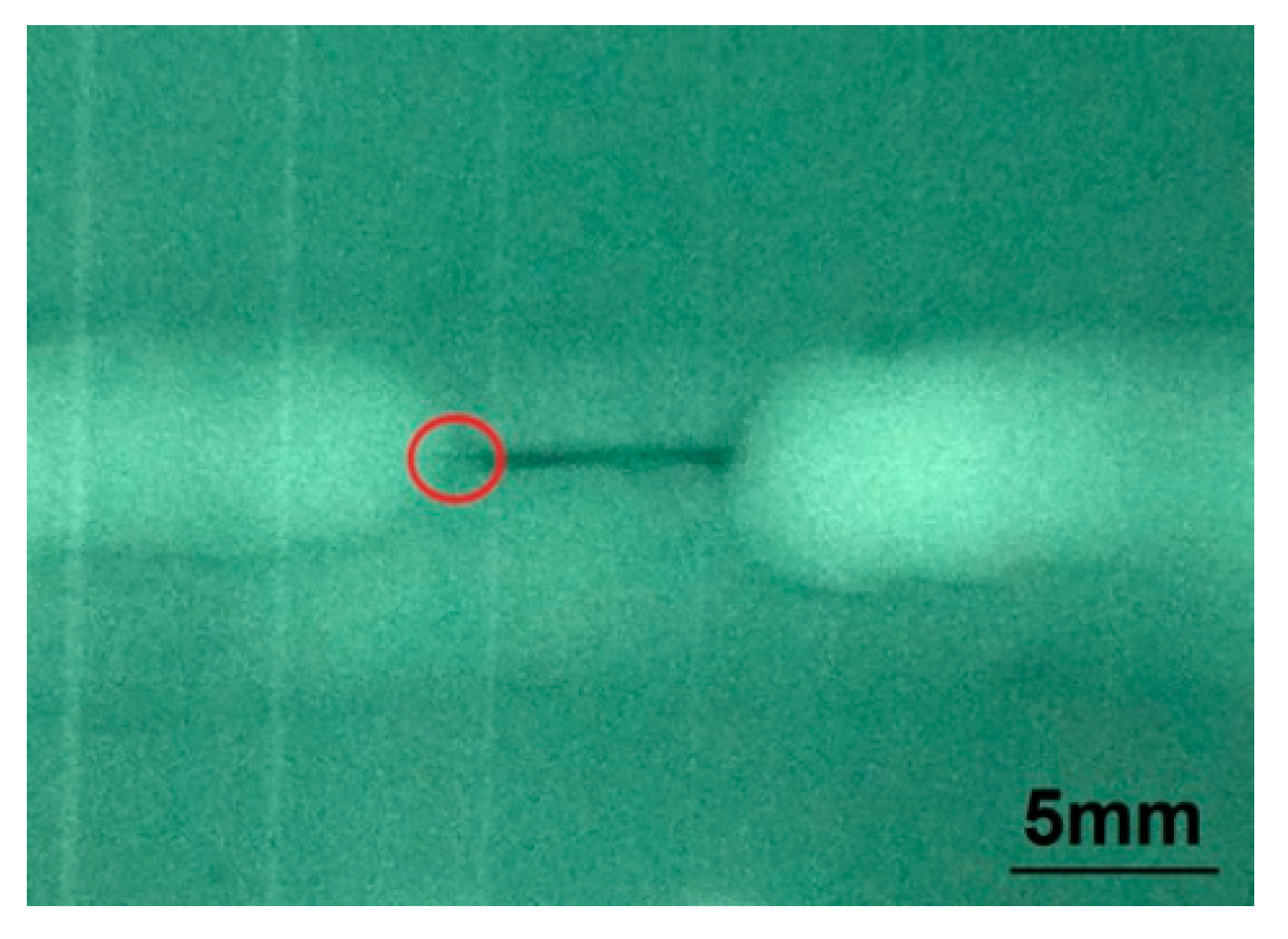
In Figure 2, the results of X-ray detection show the evolution of fatigue cracks. In Figure 2a, there is only the prefabricated defect without any fatigue cracks, i.e., the normal state. Then, the hidden crack of 1.2 mm was generated after 1280 kc, which has been marked with a circle in Figure 2b and cannot be seen with the naked eye. At last, the macroscopic crack visible to eyes appeared after 1560 kc.

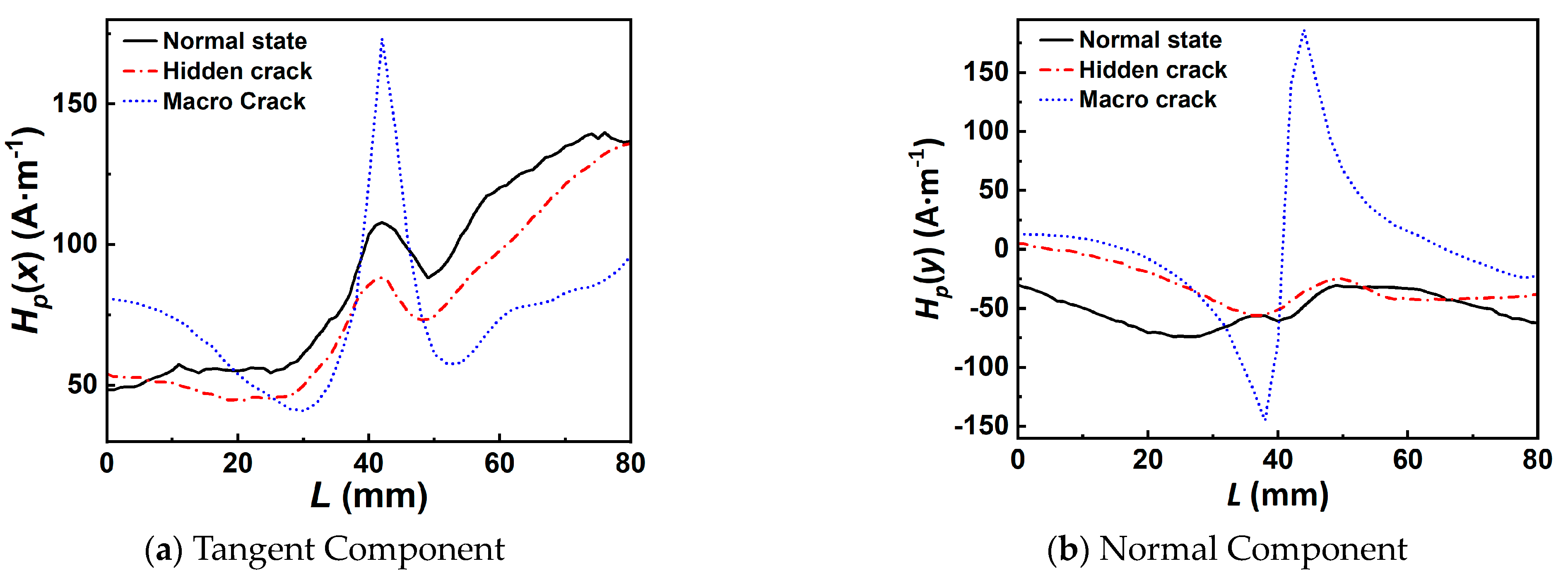
By referring to X-ray testing results, the tangential signals H_p(x) and normal component signals H_p(y) of different defect levels and their corresponding fatigue cycle numbers are extracted, as shown in Figure 3. The fluctuation of MMM tangent component H_p(x) of hidden crack state is bigger than that of the normal state, although a small jump of H_p(x) occurs on the welded joints in the normal state due to the welding residual stress in Figure 3a. The jump of H_p(x) grows higher when the hidden crack is generated. The value becomes highest when the macroscopic crack is generated. In Figure 3b, the peak-to-peak value of the normal signal component H_p(y) in weld position increases in turn from normal state to hidden crack and then to macroscopic crack, in which the defect levels can be identified by MMM curves. When macroscopic cracks are produced, the polarity varies along the normal component H_p(y) on the SCZs.

Sometimes, due to the interruption of welding residual stress, it is difficult to distinguish between the hidden crack state (1260 kc) and the normal state (0 kc) only by MMM curves shown in Figure 4. The fluctuations of H_p(x) curve in the hidden crack state are very similar to that in the normal state, as shown in Figure 4a. At the same time their curves of H_p(y) overlap with each other in Figure 4b. However, in Figure 5, the result of X-ray detection showed that there was a hidden crack of 1.8 mm on left of the prefabricated defect which has been marked with a circle when the fatigue cycles reach 1260 kc.

4. MLE MMM Modeling

The multiple parameters should be adopted comprehensively because the single MMM characteristic parameter cannot accurately determine the defect levels. For the multiple parameters estimation from the view of mathematical statistics, MLE method is well-suited.

4.1. MLE MMM Modeling

The characteristic parameters of the tangential and normal MMM signals are extracted from the experiment data.

(1) Peak-to-peak value

$$\mathrm{\Delta }{H}_p(x)=H_p^{\max }(x)-H_p^{\min }(x)$$

(1)

$$\mathrm{\Delta }{H}_p(y)=H_p^{\max }(y)-H_p^{\min }(y)$$

(2)

where ΔH_p(x) is the tangential peak-to-peak value and ΔH_p(y) is the normal one. H_p^max(x) and H_p^max(y) are the maximum values of the MMM tangential and normal magnetic induction intensity, respectively. H_p^min(x) and H_p^min(y) are the minimum values of the tangential and normal magnetic induction intensity, respectively.

(2) Gradient

$$G_x=\mathrm{d}{H}_p(x)/\mathrm{d}x$$

(3)

$$G_y=\mathrm{d}{H}_p(y)/\mathrm{d}y$$

(4)

where G_x is the tangential gradient, and G_y is the normal one.

(3) Gradient limit state coefficient

$$Z_x=G_x^{\max }/G_x^{\mathrm{ave}}$$

(5)

$$Z_y=G_y^{\max }/G_y^{\mathrm{ave}}$$

(6)

where Z_x is the tangential gradient limit state coefficient, and Z_y is the normal one. G_x^max and G_x^ave are the maximum value and average value of the tangential gradient in the testing zones, respectively. G_y^max and G_y^ave are the maximum value and average value of the normal gradient, respectively.

4.2. Kernel Density Function

In order to quantitatively establish the MLE MMM model, the probability density function needs to be built first. X₁, X₂, …, X_n are set as independent and identically distributed random variables in the space R. The probability density function of random variable X in kernel method [23] is defined as:

$$\widehat{f}=\frac{1}{nh}{\displaystyle \sum _{i=1}^{n}K\left(\frac{x-x_i}{h}\right)}$$

(7)

where K(x) is the kernel function, h is the bandwidth, x_i is sample values of X, n is the sample size, and $\widehat{f}$ presents the estimated probability density.

The experiment results show that the MMM data obey Gaussian distribution [14], so the Gauss kernel is adopted. The bandwidth h has a great impact on the result of the probability density estimation. If h is too small, the result will be unstable. Otherwise, the resolution ratio of the result is too low. So, the optimized bandwidth algorithm is adopted, which is mainly based on mean integral square error (MISE). Its formula is given in reference [24]. The optimal bandwidth is then calculated by solving the equation with the formula

$$h_{op}=\sqrt[5]{\frac{4n{h}^6}{{\displaystyle \sum _{i=1}^n{\displaystyle \sum _{j\prec i}^n\left[\frac{\sqrt{\pi }}{16h^3}\left\{{\left[{\left(x_i-x_j\right)}^2-6h^2\right]}^2-24h^4\right\}\exp \left(-\frac{{\left(x_i-x_j\right)}^2}{4h^2}\right)\right]}}}}$$

(8)

The iterative algorithm is adopted to find the most optimal bandwidth. First h₁ = h_op(h₀) and h₀ = 1.06σn^−1/5 are calculated, where n is the sample size, σ is the standard deviation of the sample observations. δ is set as a minimum value. When |h₁ − h₀| > δ, cycle steps are performed as follows:

• Assign the h₁ to the h₀, that is, h₀ = h₁;
• Bring the new h₀ into h₁ = h_op(h₀) to calculate the new h₁;
• h₁ = (h₀ + h₁)/2.

According to the above algorithm, the results of the optimized bandwidth are shown in

Table 3. Results of optimized bandwidth.

ΔHp(x)	Gxmax	Zxmax	ΔHp(y)	Gymax	Zymax
8.046	1.9236	0.1421	6.9817	1.8659	0.2482

.

Then, the kernel functions of six MMM characteristic parameters can be obtained, which are ${\widehat{f}}_{\mathrm{\Delta }{H}_p(x)}$, ${\widehat{f}}_{G_x^{\max }}$, ${\widehat{f}}_{Z_x^{\max }}$, ${\widehat{f}}_{\mathrm{\Delta }{H}_p(y)}$, ${\widehat{f}}_{G_y^{\max }}$, ${\widehat{f}}_{Z_y^{\max }}$. These functions form the probability density database of the MMM characteristic parameters. And they are brought into the six kernel density functions to calculate the probability density in the database. The kernel density function is integrated in order to obtain the probability.

4.3. MLE MMM Modeling

The six MMM parameters above contain damage information from different levels. On the basis of the experiment data, these characteristic values are divided into three defect levels, which are normal state, hidden crack state and macroscopic crack state. Considering X-ray detection was taken as the basis comparison of MMM testing experiments, the three defect levels are defined, compared with the current quantitative standards of X-ray detection NB/T 47013.2–2015 and SY/T 4109–2020. In the X-ray detection standards, level I is defined as normal and no defects, level II is defined as the defect length is less than T/3, and level III is specified as the defect length is less than 2T/3, in which T is the nominal thickness of the base metal. The normal state in this paper is consistent with level I of the X-ray detection standard. The hidden crack state, where cracks are invisible to the naked eye and less than 2 mm (T/3) in length, is equivalent to level II of the X-ray detection standard. The macroscopic crack state, where cracks are visible to the naked eye and greater than 2 mm in length, corresponds to level III in the X-ray detection standard. Here, 2 mm only refers to the length of the fatigue crack generated from the end of the prefabricated lack of penetration. The classification standard in this paper is stricter than the X-ray detection standard in order to reflect the advantages of MMM in early damage detection.

From the view of MLE [25], if the total X is discrete, its distribution law is P{X = x} = p(x;θ), θ∈Θ. Here, θ is the estimated parameter, Θ is the possible range of θ. x₁, x₂, …, x_n are set as sample values of X₁, X₂, …, X_n. Then, the probability of the incidents {X₁ = x₁, X₂ = x₂, …, X_n = x_n} is

$$L(\theta )=L(x_1,x_2,..,x_n;\theta )={\displaystyle \prod _{i=1}^{n}p(x_i;\theta ),\theta \in \Theta }$$

(9)

where L(θ) is the likelihood function.

The MLE estimation models based on MMM characteristic parameters are:

$$L_x={\displaystyle \prod _{i=1}^n{p}_x\left(x_i\right)=p\left(\mathrm{\Delta }{H}_p\left(x\right)\right)\cdot p\left(G_x^{\max }\right)}\cdot p\left(Z_x^{\max }\right)$$

(10)

$$L_y={\displaystyle \prod _{i=1}^n{p}_y\left(x_i\right)=p\left(\mathrm{\Delta }{H}_p\left(y\right)\right)\cdot p\left(G_y^{\max }\right)}\cdot p\left(Z_y^{\max }\right)$$

(11)

where L_x and L_y are the MLE values of the tangential and normal signals, respectively. p_x(x_i) and p_y(x_i) are the probability of x_i based on optimized bandwidth kernel density estimation, respectively.

The MLE probabilities of three defect levels, which are, normal state, hidden crack and macroscopic crack, are shown in Figure 6. The mathematical expectation values of the MLE probability are calculated through mathematical statistics.

In this paper, 100 specimens were divided into 10 groups during the fatigue tensile experiments. Each specimen was scanned and the MMM signals were recorded every 20 kilocycles, and 6 characteristic values of each signal curve were extracted. On average, more than 50 sets of data were recorded for each specimen. In total, over 30,000 characteristic values were recorded, along with the corresponding fatigue cycles and defect levels. The Gauss kernel probability density functions of the three defect levels were established based on the database of 30,000 characteristic values. Then, the mathematical expectation values of MLE probability in

Table 4. Mathematical expectation of MLE probability.

Mathematical Expectation	Tangential Signal	Normal Signal
Normal state	0.05	0.09
Hidden crack	0.18	0.17
Macroscopic crack	0.41	0.48

were obtained by integrating the Gauss kernel probability density functions for each defect level.

It can be seen in Figure 6 that the three damage states can be mostly identified, but there is still partial overlap. Considering that the D–S theory is capable of dealing with uncertain information for small sample data, D–S theory is introduced to modify the above MLE MMM model in order to increase identification accuracy.

5. Modified MLE MMM Model Based on D–S Theory

5.1. MLE Value Neartude

In order to identify the defect levels of welded joints using the D–S evidence theory, the identified framework should be set first. The propositions of the identified framework are the three defect levels which constitute the feature vector. d_ij is the distance between MLE probability of the unknown defect level and the mathematical expectation of two MMM signal directions. t_ij is proximity. The formulas are as follows:

$$d_{ij}=\left|A_{ij}-E_j\right|$$

(12)

$$t_{ij}=1-\frac{d_{ij}^2}{d_{1j}^2+d_{2j}^2+d_{3j}^2}$$

(13)

where E_j is an unknown defect level of different MMM signal directions. A_ij is the mathematical expectation.

5.2. Reliability Function

Assuming that there is a target to identify, Θ represent all the possible results for the identifying target, and all the possible results are called hypothesis [26]. Θ is set as an identified framework if the set function m:2^Θ→[0, 1] meet the following requirements:

$$m\left(\phi \right)=0$$

(14)

$${\displaystyle \sum _{A\subset \Theta }m\left(A\right)}=1$$

(15)

m is known as the basic reliability allocation (Mass function) of the identified framework. The Formula (14) means no reliability is produced for the empty proposition, and Formula (15) reflects that the sum of all the proposition’s reliability is 1. A is called focal element when m > 0 [27]. The m(A) is the basic reliability of subset A, which represents the reliability degree of subset A. For any proposition sets, the reliability function Bel is defined as:

$$Bel(A)={\displaystyle \sum _{B\subset A}m(B)}$$

(16)

B is an element of subset A. In this paper, subset A is selected as the weld defect level set, and B is the normal state, hidden crack and macroscopic crack.

5.3. Basic Reliability Function Allocation

The basic reliability allocation function m_ij and uncertainty m_j(Θ) of each proposition in the identified framework are as follows:

$$m_{ij}=\frac{t_{ij}}{S-1}(1-R_i)$$

(17)

$$m_j(\Theta )=R_i$$

(18)

where R_i = b_i·μ_i represents the overall uncertainty whilst identifying the defect level, and μ_i is the uncertainty of MLE probabilities as evidence body in the framework, which can be given by expert opinion or data statistics of the experiment, 0.1 is taken. S = 3 represents three defect levels.

$$b_i=\sqrt{\frac{1}{2}{\displaystyle \sum _{\begin{array}{l}j=1\\ j\ne m\end{array}}^3{(t_{ij}-u_i)}^2}}$$

(19)

$$u_i=\frac{1}{2}{\displaystyle \sum _{\begin{array}{l}j=1\\ j\ne m\end{array}}^3{t}_{ij}}$$

(20)

where b_i is the variance of the proximity except for the biggest proximity of the proposition close to the unknown defect level. And u_i is the mean value of the proximity except for the biggest proximity of the proposition that is close to the unknown defect level.

5.4. D–S Information Fusion

(1) Two Reliability Functions Fusion

Bel₁ and Bel₂ are two reliability functions of the same target framework set, m₁ and m₂ are the basic reliability allocation of function Bel₁ and Bel₂, respectively. MLE probabilities of the tangential and normal MMM characteristic value are selected as the Bel₁ and Bel₂. C and D represent the defect levels of tangential and normal signals, respectively.

$${\displaystyle \sum _{C_i\cap D_j=\phi }{m}_1(C_i)m_2(D_j)}<1$$

(21)

Then, the basic reliability allocation is:

$$m(C)=\{\begin{array}{cc}0& C=\phi \\ \frac{{\displaystyle \sum _{C_i\cap D_j=C}{m}_1(C_i)m_2(D_j)}}{1-k}& C\ne \phi \end{array}$$

(22)

$$k=\left({\displaystyle \sum _{C_i\cap D_j=\phi }{m}_1\left(C_i\right)m_2\left(D_j\right)}\right)$$

(23)

where k represents the inconsistency factor. i, j = 1, 2, 3 represent the level of defect levels, which are: 1 is normal state, 2 is hidden crack state and 3 is macroscopic crack state.

(2) Decision rules of D–S theory

$$m(C_1)=\max (m(C_i),C\subset \Theta )$$

(24)

$$m(C_2)=\max (m(C_i),C\subset \Theta ,C_i\ne C_1)$$

(25)

$$\{\begin{array}{l}m(C_1)-m(C_2)>{\epsilon }_1\\ m(\Theta )<{\epsilon }_2\\ m(C_1)>m(\Theta )\end{array}$$

(26)

The recognition result is C1 when meeting the conditions of Formulas (24) to (26), where m(Θ) is the uncertainty degree, and ε₁ and ε₂ are set as threshold value.

6. Validation

Under the same experimental conditions, thirty specimens of unknown weld defect levels had been selected to verify the modified MLE MMM model based on the D–S theory. Take specimen 17 as an example, after 980 fatigue kilocycles, the specimen, which showed no macroscopic crack visible to the naked eye, was examined by X-rays. The result of X-ray detection showed that there were no hidden cracks on both sides of the prefabricated defect shown in Figure 7.

Then, by analyzing the MMM data, the tangential and normal components of ΔH_p, G and Z are (28.9, 5.75, 2.441) and (9.6, 6.5, 5.007), respectively. Then, the tangential and normal MLE probabilities are calculated, respectively, by Formulas (10) and (11), the results are 0.16 and 0.12. The proximity of the unknown defect level are obtained by Formulas (12) and (13), and the results are listed in

Table 5. MLE probability proximity of the identifying damage state.

Proximity	Tangential Signal	Normal Signal
Normal state	0.84	0.99
Hidden crack	0.99	0.98
Macroscopic crack	0.17	0.03

. Then, the basic reliability allocation is calculated by Formulas (17) and (18), shown in

Table 6. Basic reliability allocation of the identifying damage state.

Basic Reliability Allocation	Tangential Signal	Normal Signal
Normal state	0.47	0.41
Hidden crack	0.47	0.48
Macroscopic crack	0.01	0.08
Uncertainty degree	0.047	0.033

.

It can be seen that the basic reliability allocations of the normal and hidden crack are similar. It is still difficult to identify the unknown defect level only based on the basic reliability allocation. So, it is necessary to use the information fusion. The information fusion results are listed in

Table 7. Information fusion results.

	mbel1 = D1(0.41)	mbel1 = D2(0.48)	mbel1 = D3(0.08)	mbel1 = Θ(0.033)
mbel2 = C1(0.47)	C1(0.1927)	Φ(0.2256)	Φ(0.0376)	C1(0.01551)
mbel2 = C2(0.47)	Φ(0.1927)	C2(0.2256)	Φ(0.0376)	C2(0.01551)
mbel2 = C3(0.01)	Φ(0.0041)	Φ(0.0048)	C3(0.0008)	C3(0.00033)
mbel2 = Θ(0.047)	C1(0.01927)	C2(0.02256)	C3(0.00376)	Θ(0.00155)

.

The inconsistency factor k is calculated by Formula (23), and the result is as follows:

k = 0.2256 + 0.04 + 0.0376 + 0.1458 + 0.1927 + 0.0376 + 0.0041 + 0.0048 = 0.5024

So, the basic reliability allocation of the evidence Bel₁ and Bel₂ is calculated by Formula (22). And the reliability allocation after information fusion is shown in

Table 8. Reliability allocation of information fusion.

Reliability	m (Tangential Normal)
Normal state	0.46
Hidden crack	0.53
Macroscopic crack	0.0098
mj(Θ)	0.003

.

According to the decision rules of the D–S theory, ε₁ and ε₂ are taken as 0.01 and 0.001, then the prediction result is hidden crack. The results show the reliability is 53% and uncertainty degree m(Θ) is 0.3%.

In order to determine the unknown defect level from the experimental point of view, a scanning electron microscopy (SEM) has been applied to test the selected specimen. At the end of the prefabricated defect, the wire-electrode cutting was used to obtain the SEM specimen as shown in the dashed box in Figure 8. The cutting surface 1 is the SEM observation surface with the length of 15 mm. The distance from the cutting surface 2 to 1 was 10 mm.

The SEM result is shown in Figure 9. Some hidden cracks circled by ellipses with a size of about 0.25 mm have appeared in Figure 9. This result is consistent with the predictions of the modified MLE MMM model, which shows that the modified MLE MMM model can identify hidden crack damage earlier than X-ray detection. The other 29 specimens have the same verification process as specimen 17. The smallest uncertainty degree is 0.30%, the largest one is 7.09%, and the average one is 3.66%, as shown in Figure 10. The results verify the validity of the modified MLE MMM model based on the D–S theory.

7. Conclusions

(1) Due to the existence of welding residual stress, it is difficult to distinguish between the normal state and the hidden crack state. At the same time, considering that a single MMM feature parameter cannot accurately reflect the level of welding defects, it is necessary to extract multiple MMM feature parameters, namely ΔH_p(x), G_x^max, Z_x^max, ΔH_p(y), G_y^max and Z_y^max for quantitative identification;

(2) The different defect levels, that is, normal state, hidden crack and macroscopic crack, can be identified based on the MLE MMM model from mathematical statistics. But there exists a partial overlap between normal state and hidden crack state. So, the modified MLE MMM model based on the D–S theory is presented, of which the smallest uncertainty degree is 0.3%, the largest one is 7.09%, and the average one is 3.66%;

(3) The validation results are consistent with the prediction result of the modified MLE MMM model based on D–S theory. It shows that the modified model is effective in distinguishing early hidden cracks from welding residual stress, which is earlier than X-ray detection. The method is suitable for ferromagnetic materials such as Q235B and Q345. This provides a new tool of MMM quantitative identification for weld defect levels.

References

- Jambor, M.; Pokorny, P.; Trsko, L.; Oplt, T.; Jackova, M.; Hutar, P. Microstructure and the fatigue crack propagation in the dissimilar low alloy/stainless steel GMAW welded joints. Mater. Charact. 2022, 191, 112119. [Google Scholar] [CrossRef]
- Wang, X.J.; Meng, Q.C.; Hu, W.P. Fatigue life prediction for butt-welded joints considering weld-induced residual stresses and initial damage, relaxation of residual stress, and elasto-plastic fatigue damage. Fatigue Fract. Eng. Mater. Struct. 2019, 42, 1373–1386. [Google Scholar] [CrossRef]
- Su, S.Q.; Yang, Y.Y.; Wang, W.; Ma, X.P. Crack propagation characterization and statistical evaluation of fatigue life for locally corroded bridge steel based on metal magnetic memory method. J. Magn. Magn. Mater. 2021, 536, 168136. [Google Scholar] [CrossRef]
- Bao, S.; Jin, P.F.; Zhao, Z.Y.; Fu, M.L. A Review of the Metal Magnetic Memory Method. J. Nondestruct. Eval. 2020, 39, 11. [Google Scholar] [CrossRef]
- Moonesan, M.; Kashefi, M. Effect of Sample Initial Magnetic Field on the Metal Magnetic Memory NDT Result. J. Magn. Magn. Mater. 2018, 460, 285–291. [Google Scholar] [CrossRef]
- Ozhigov, L.S.; Mitrofanov, A.S.; Dobrovol’skaya, I.Y.; Shramchenko, S.V.; Vasilenko, R.L.; Rybal’chenko, N.D.; Krainyuk, E.A. Corrosion Defects in Pipelines of Nuclear Power Plants and the Problems of Their Inspection. Mater. Sci. 2018, 53, 777–782. [Google Scholar] [CrossRef]
- Wang, H.P.; Dong, L.H.; Wang, H.D.; Ma, G.Z.; Xu, B.S.; Zhao, Y.C. Effect of tensile stress on metal magnetic memory signals during on-line measurement in ferromagnetic steel. NDT E Int. 2020, 117, 102378. [Google Scholar] [CrossRef]
- Kashefi, M.; Clapham, L.; Krause, T.W.; Underhill, P.R.; Krause, A.K. Stress-Induced Self-Magnetic Flux Leakage at Stress Concentration Zone. IEEE Trans. Magn. 2021, 57, 6200808. [Google Scholar] [CrossRef]
- Dubov, A.; Dubov, A.; Kolokolnikov, S. Detection of local stress concentration zones in engineering products-the lacking link in the non-destructive testing system. Weld. World 2018, 62, 301–309. [Google Scholar] [CrossRef]
- Shi, P.P.; Hao, S. Analytical solution of magneto-mechanical magnetic dipole model for metal magnetic memory method. Acta Phys. Sin. 2021, 70, 034101. [Google Scholar] [CrossRef]
- Avakian, A.; Ricoeur, A. An extended constitutive model for nonlinear reversible ferromagnetic behaviour under magnetomechanical multiaxial loading conditions. J. Appl. Phys. 2017, 121, 053901. [Google Scholar] [CrossRef]
- Ni, C.; Hua, L.; Wang, X.K. Crack propagation analysis and fatigue life prediction for structural alloy steel based on metal magnetic memory testing. J. Magn. Magn. Mater. 2018, 462, 144–152. [Google Scholar] [CrossRef]
- Yao, K.; Wu, L.B.; Wang, Y.S. Nondestructive Evaluation of Contact Damage of Ferromagnetic Materials Based on Metal Magnetic Memory Method. Exp. Tech. 2019, 43, 273–285. [Google Scholar] [CrossRef]
- Xu, K.S.; Yang, K.; Liu, J.; Wang, Y. Study on metal magnetic memory signal of buried defect in fracture process. J. Magn. Magn. Mater. 2020, 498, 166139. [Google Scholar] [CrossRef]
- Liu, B.; Lian, Z.; Liu, T.; Wu, Z.H.; Ge, Q. Study of MFL signal identification in pipelines based on non-uniform magnetic charge distribution patterns. Meas. Sci. Technol. 2023, 34, 044003. [Google Scholar] [CrossRef]
- Liu, B.; Luo, N.; Feng, G. Quantitative Study on MFL Signal of Pipeline Composite Defect Based on Improved Magnetic Charge Model. Sensors 2021, 21, 3412. [Google Scholar] [CrossRef]
- Xing, H.Y.; Dang, Y.B.; Wang, B.; Leng, J.C. Quantitative Metal Magnetic Memory Reliability Modeling for Welded Joints. Chin. J. Mech. Eng. 2016, 29, 372–377. [Google Scholar] [CrossRef]
- Xing, H.Y.; Xu, C.; Liu, C. Characterization of Physical Short Crack Growth at the Meso-scale Based on Magnetic Property Parameters. Adv. Eng. Sci. 2023, 55, 307–314. [Google Scholar] [CrossRef]
- JB/T 4730-2005; Nondestructive Testing of Pressure Equipments. Xinhua Publishing House of China: Beijing, China, 2010.
- Ren, S.K.; Ren, X.Z.; Duan, Z.X.; Fu, Y.W. Studies on influences of initial magnetization state on metal magnetic memory signal. NDT E Int. 2019, 103, 77–83. [Google Scholar] [CrossRef]
- Chen, H.L.; Wang, C.L.; Zuo, X.Z. Research on methods of defect classification based on metal magnetic memory. NDT E Int. 2017, 92, 82–87. [Google Scholar] [CrossRef]
- GB/T 3075-2008; Metallic Materials—Fatigue Testing—Axial-Force-Controlled Method. Standards Press of China: Beijing, China, 2010.
- Arora, S.; Taylor, J.W. Forecasting electricity smart meter data using conditional kernel density estimation. Omega-Int. J. Manag. Sci. 2016, 59, 47–59. [Google Scholar] [CrossRef] [Green Version]
- Davies, T.M.; Baddeley, A. Fast computation of spatially adaptive kernel estimates. Stat. Comput. 2018, 28, 937–956. [Google Scholar] [CrossRef]
- Yamamura, K. Bayes estimates as an approximation to maximum likelihood estimates. Popul. Ecol. 2016, 58, 45–52. [Google Scholar] [CrossRef]
- Can, C.E.; Ergun, G.; Soyer, R. Bayesian Analysis of Proportions via a Hidden Markov Model. Methodol. Comput. Appl. Probab. 2022, 24, 3121–3139. [Google Scholar] [CrossRef]
- Cao, L.X.; Liu, J.; Han, X.; Jiang, C.; Liu, Q.M. An efficient evidence-based reliability analysis method via piecewise hyperplane approximation of limit state function. Struct. Multidiscip. Optim. 2018, 58, 201–213. [Google Scholar] [CrossRef]