Robust Trajectory Tracking Control for Constrained Small Fixed-Wing Aerial Vehicles with Adaptive Prescribed Performance

Featured Application

The low complexity of the proposed controller along with the adaptive performance characteristics and the robustness against external disturbances could lead to implementation as longitudinal motion autopilot in small fixed-wing UAVs.

Abstract

A novel approximation-free adaptive prescribed performance control scheme for the longitudinal motion tracking of input and state constrained small fixed-wing UAVs is designed in this work. The proposed controller employs the adaptive prescribed performance technique to impose output performance specifications in accordance with actuation limitations regarding the amplitude and the rate of the control signal. Furthermore, state constraints are introduced to ensure the proper operation of the closed-loop system. The adoption of PPC methodology results in a low complexity control algorithm with easy gain selection which facilitates its practical implementation. Finally, a comprehensive simulation study as well as comparative simulation paradigms on an Aerosonde model clarifies and verifies the superiority and the effectiveness of the proposed controller to control the longitudinal motion of UAVs in the presence of wind gusts.

1. Introduction

An unmanned aerial vehicle (UAV) is a space-traversing vehicle capable of flying without a human crew on board and can be remotely controlled or operate autonomously [1]. During the last few decades, UAVs have gained significant attention in civilian domains, surpassing their traditional association with military and defense applications. Particularly, such systems are now extensively exploited in various sectors, including precision agriculture [2,3,4], construction industry [5], air taxis, and merchandise delivery [6]. In the vein of those applications, a commonly arising problem is the design of an effective feedback controller such that the closed-loop system tracks a desired reference altitude and airspeed velocity. For example, consider a scenario where a user intends to manually command a UAV to fly over a forest area for the purpose of detecting potential wildfires. Manual control of the UAV presents difficulties as it requires applying complex control inputs, such as roll, pitch, or/and yaw commands, to maintain the vehicle’s desired cruising speed along a predefined trajectory, even without the presence of external disturbances. Thus, the exploitation of automatic control techniques becomes indispensable in order to overcome the limitation of manual operation and ensure precise and safe maneuvering of the UAV.

One of the most commonly used controllers in autopilots, is the PID because of its implementation simplicity and low computational burden [7,8]. Moreover, approximation-based techniques utilized in autopilots include fuzzy logic [9] and neural network algorithms [10] that estimate the model of the UAV, at the expense of computational complexity of the control scheme. An alternative approach is to approximate their dynamics using linear models. One effective method to enhance altitude control performance is to exploit Linear Quadratic Gaussian controllers [11]. Furthermore, ${\mathcal{H}}_{\infty }$ loop-shaping methods can be applied to small fixed-wing UAVs, especially in situations involving noise or varying payload conditions, to achieve improved control performance [12]. A novel system-decomposition-based robust control method for linearized fixed-wing UAVs is introduced in [13]. By decomposing the system into simpler subsystems, the controller design becomes easier and the overall complexity is reduced. In particular, each subsystem utilizes an extended state-observer-based robust control method to enhance tracking performance and handle disturbances. Alternatively, the authors in [14] proposed a feedback linearization control scheme dealing with the nonlinear equations of motion. Nevertheless, a precise model of the system is required. In aircraft flight control, the aerodynamic forces and moments acting on the aircraft are nonlinear functions that cannot be modeled exactly and thus achieving perfect cancellation of such nonlinearities becomes unattainable. Consequently, there are inherent limitations associated with employing exact state feedback linearization, particularly when confronted with unmodeled dynamics and uncertainties in system parameters. Furthermore, Model Predictive Control (MPC) is commonly employed to address the trajectory tracking problem [15,16,17]. Although, MPC is a method with great applications, mainly in slowly evolving systems, the computational burden associated with their iterative nature should be taken into consideration during their practical implementation in fast dynamical systems such as UAVs. Backstepping is another well-studied nonlinear technique in the related literature [18,19,20]. An adaptive backstepping flight controller for a high-performance UAV was designed in [21], addressing various constraints such as saturations, bandwidth limitations, and rate limits which are encountered in all practical control systems. To facilitate the control design, a linear aerodynamic model was employed in addition to adaptation laws integrated into the system in order to enable online estimation of the stability derivatives within the model.

The control inputs of UAVs, as in all physical systems, are subjected to several constraints rising from the external environment, mechanical limitations, and energy restrictions. It is crucial to take these control constraints into account during the design and implementation of control systems. In practical scenarios, physical actuation limitations inevitably arise, introducing constraints in both the amplitude and the slew rate of the control input. These constraints can significantly impact the overall performance of the closed-loop system, potentially leading to undesired inaccuracies or even instability. A constrained nonlinear tracking controller for small fixed-wing kinematic UAVs was designed in [22]. The proposed algorithm involves the construction of control input that adhere to a predefined control Lyapunov function (CLF). From this set, a guidance law is selected to facilitate trajectory tracking. Moreover, the nested saturation technique to convert control input constraints into command angle constraints was presented in [23]. Recently, a backstepping control scheme providing trajectory tracking for an input constrained spacecraft was proposed in [24], exploiting a second-order anti-windup model.

Owing to its inherent light-weight structure, the fixed-wing UAV is susceptible to the influence of external wind disturbances, which induce significant undesirable effects on trajectory tracking performance and may lead to instability. Thus, the disturbance rejection capability of fixed-wing UAV system is one of the most crucial factors to be considered when designing the controller. Methods to estimate the unknown external disturbances involve the utilization of $L_1$ adaptive augmentation [25] and the disturbance observer based control (DOBC) approach [26,27]. Thus, it is critical for the flight control scheme to be robust in order to achieve stable flights in realistic conditions.

A robust nonlinear control technique introduced in [28] and further extended in approximation-free approach in [29], known as Prescribed Performance Control (PPC), guarantees the evolution of the tracking error within a user-prespecified performance envelope for bounded control input. In this vein, PPC is a robust control technique that imposes predefined transient and steady-state tracking characteristics to nonlinear systems. A PPC based control scheme for the trajectory tracking of small fixed-wing UAVs was recently presented in [30]. However, this algorithm does not take into account input constraints, which renders the practical implementation rather difficult, as any steady state perturbation may lead the system to singularity (the closed-loop signals become unbounded) as the saturated control effort fails to maintain the tracking error within the conventional prescribed envelope. Recently, input constrained issues have been addressed in [31,32] within the approximation-free PPC framework, where an adaptive PPC (APPC) scheme counteracts input limitations by properly modifying the output constraints (i.e., the tracking error specifications), depending on the feasible control effort that can be applied to the plant.

In this work, motivated by the above discussion, we aim at designing a novel robust scheme for the trajectory tracking control of the longitudinal motion of small fixed-wing UAVs subject to input and state constraints with guaranteed adaptive prescribed performance specifications. In particular, the main contribution of this work is the development of a control scheme that exhibits the following features:

• Addresses, for the first time, output prescribed performance specifications in accordance with input constraints both on amplitude and the rate of the control signals, and guarantees the boundedness of the closed-loop signals;
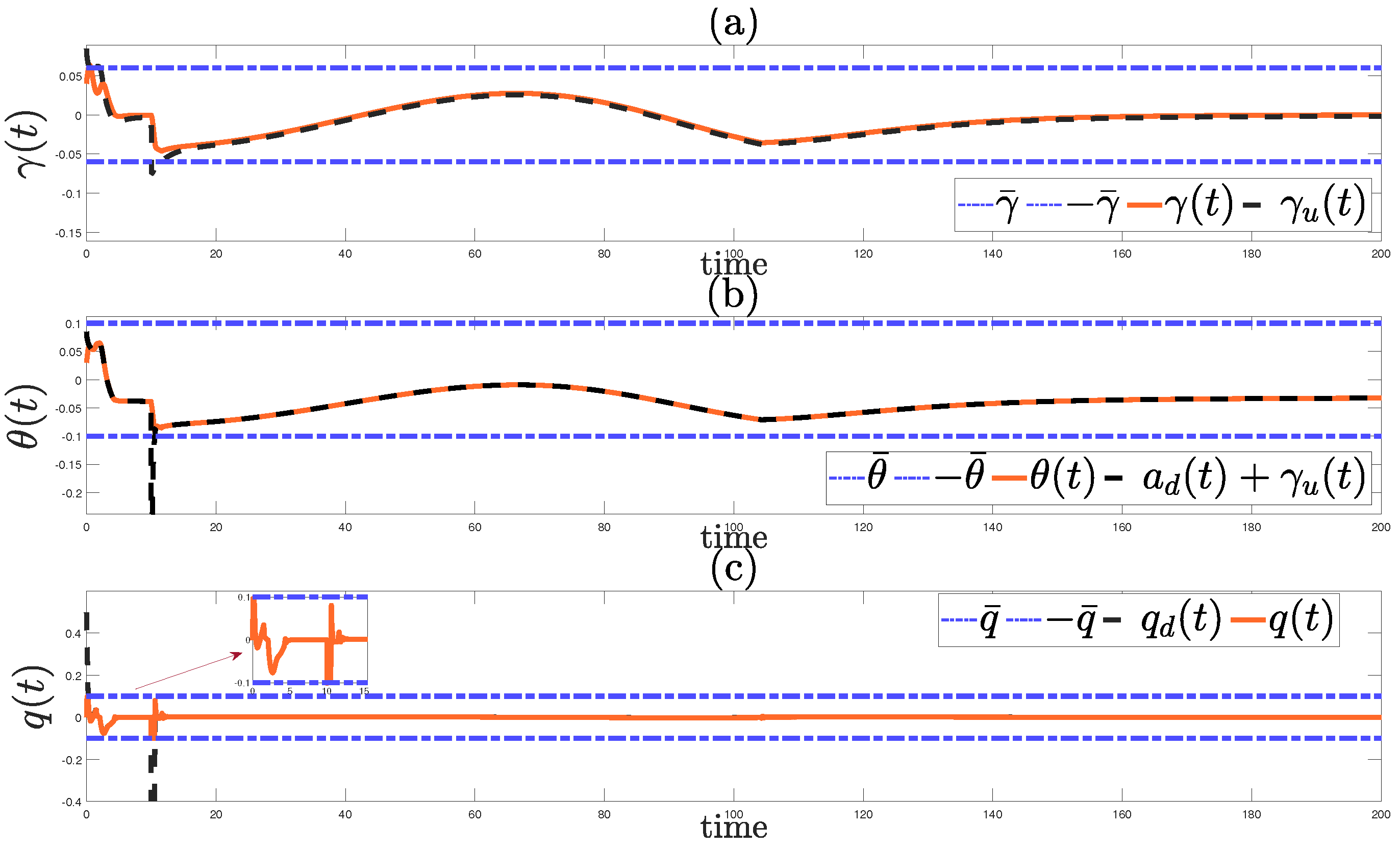
• Unlike most of the related works, imposes prescribed state constraints, by combining APPC approach and saturating the generated state reference trajectories of flight-path-angle, pitch angle, angle-of-attack and pitch rate in order to navigate the UAV efficiently, avoiding destabilizing phenomena such as stall;
• Is approximation-free, thus does not require either knowledge of the system nonlinearities as in [9,10,11,12,13,14,15,16,17,24] or any disturbance observer as in [25,26,27]. Additionally, the gain tuning constitutes a straightforward task in contrast with [7,8] and the complexity of the resulted robust controller is low, which facilitates the implementation as motion autopilot in small fixed-wing UAVs.

2. Problem Formulation and Preliminaries

The longitudinal flight dynamics of a small fixed-wing UAV in the presence of wind disturbances is described as in [27,33] by:

$$\begin{array}{cc}\hfill \dot{h}\left(t\right)& =V\left(t\right)sin\gamma \left(t\right)+w_h\left(t\right)\hfill \end{array}$$

(1)

$$\begin{array}{cc}\hfill \dot{V}\left(t\right)& =\frac{T({\delta }_T,V)cosa\left(t\right)-D(a,V)}{m}-gsin\gamma \left(t\right)-cos\left(\gamma \right(t\left)\right){\dot{w}}_x\left(t\right)-sin\left(\gamma \right(t\left)\right){\dot{w}}_h\left(t\right)\hfill \end{array}$$

(2)

$$\begin{array}{cc}\hfill \dot{\gamma }\left(t\right)& =\frac{T({\delta }_T,V)sina\left(t\right)+L(a,V,{\delta }_e)}{mV\left(t\right)}-\frac{(g+{\dot{w}}_h\left(t\right))cos\gamma \left(t\right)}{V\left(t\right)}+\frac{sin\left(\gamma \right(t\left)\right)}{V\left(t\right)}{\dot{w}}_x\left(t\right)\hfill \end{array}$$

(3)

$$\begin{array}{cc}\hfill \dot{\theta }\left(t\right)& =q\left(t\right)\hfill \end{array}$$

(4)

$$\begin{array}{cc}\hfill \dot{q}\left(t\right)& =\frac{M(a,V,{\delta }_e,q)}{I_{yy}}\hfill \end{array}$$

(5)

where $h\left(t\right)$ denotes the altitude; $V\left(t\right)$ is the airspeed vehicle velocity; $\gamma \left(t\right)$ and $\theta \left(t\right)$ correspond to the flight-path and pitch angle, respectively; and $q\left(t\right)$ is the pitch rate with the angle-of-attack given by $a\left(t\right)=\theta \left(t\right)-\gamma \left(t\right)$. The acceleration values of the wind along with the horizontal and vertical axis are denoted by ${\dot{w}}_x\left(t\right),{\dot{w}}_h\left(t\right)$, respectively. Furthermore, the external lift, drag, pitch and thrust moments are expressed as:

$$\begin{array}{cc}\hfill L(a,V,{\delta }_e)& =\frac{1}{2}\rho V^{2}S\left(C_{L_0}+C_{L_a}a+C_{L_{{\delta }_e}}{\delta }_e\right)\hfill \\ \hfill D(a,V)& =\frac{1}{2}\rho V^{2}S\left(C_{D_0}+C_{D_a}a\right)\hfill \\ \hfill M(a,V,{\delta }_e,q)& =\frac{1}{2}\rho V^{2}S\overline{c}\left(C_{M_0}+C_{M_a}a+C_{M_q}\frac{\overline{c}}{2V}q+C_{M_{{\delta }_e}}{\delta }_e\right)\hfill \\ \hfill T({\delta }_T,V)& =\frac{1}{2}\rho S_{prop}{C}_{prop}\left[{\left(k_m{\delta }_T\right)}^2-V^2\right].\hfill \end{array}$$

Assuming a flight occurring within a vertical plane above a flat Earth, we establish a fixed coordinate system on the ground as the inertial reference frame. The coordinates of the aircraft as well as the axes of the wind gusts are illustrated in Figure 1. The control input consists of the throttle setting ${\delta }_T\left(t\right)$ and the elevator deflection ${\delta }_e\left(t\right)$. Both control signals are amplitude constrained, i.e., ${\delta }_T\left(t\right)\le {\overline{\delta }}_T$ for a positive constant ${\overline{\delta }}_T\le 1$ and $\parallel {\delta }_e\left(t\right)\parallel \le {\overline{\delta }}_e$ for a positive constant ${\overline{\delta }}_e$. Owing to the engine dynamics, the throttle command is also rate constrained, that is, $\parallel {\dot{\delta }}_T\left(t\right)\parallel \le \overline{r}$, and thus the actual throttle setting is given by:

$${\dot{\delta }}_T\left(t\right)=\varphi \left(t\right),\in [-\overline{r},\overline{r}]$$

(6)

where $\varphi \left(t\right)$ denotes a control signal to be designed. Moreover, the states of the system need to be constrained within some safety bounds. The inherent properties of fixed-wing UAVs impose limitations on angle-of-attack owing to the stall phenomenon and saturated heading rate due to pitch-rate constraints. Thus, the nonlinear system ((1)–(6)) can be written in compact form as:

$$\dot{x}=f\left(x\right)+g\left(x\right)u+z\left(x\right)d\left(t\right)$$

(7)

where $x:={[h\left(t\right),V\left(t\right),\gamma \left(t\right),\theta \left(t\right),q\left(t\right),{\delta }_T\left(t\right)]}^T$ denotes the state vector, $u:={[\varphi \left(t\right),{\delta }_e\left(t\right)]}^T$ is the control input, and $d\left(t\right):={[w_h\left(t\right),{\dot{w}}_x\left(t\right),{\dot{w}}_h\left(t\right)]}^T$ contains the disturbance components. The output of the system is chosen to be the vector $y:={[h\left(t\right),V\left(t\right)]}^T$. In this work, assuming no prior knowledge on the system dynamics $f\left(x\right),g\left(x\right),z\left(x\right)$, and the external wind disturbances d(t), we aim at designing an approximation-free, state feedback controller for the constrained system (7) that meets the following properties:

• The states of the system are constrained within a compact set.
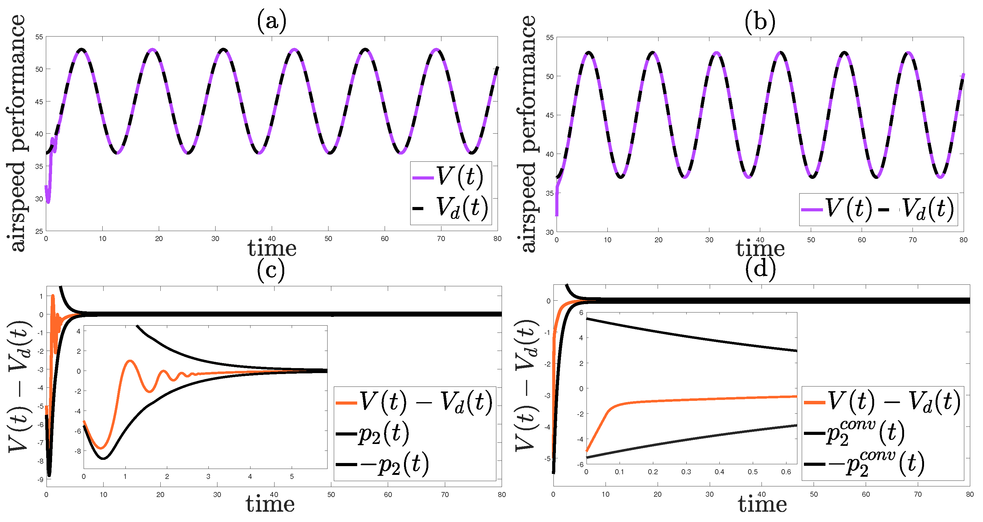
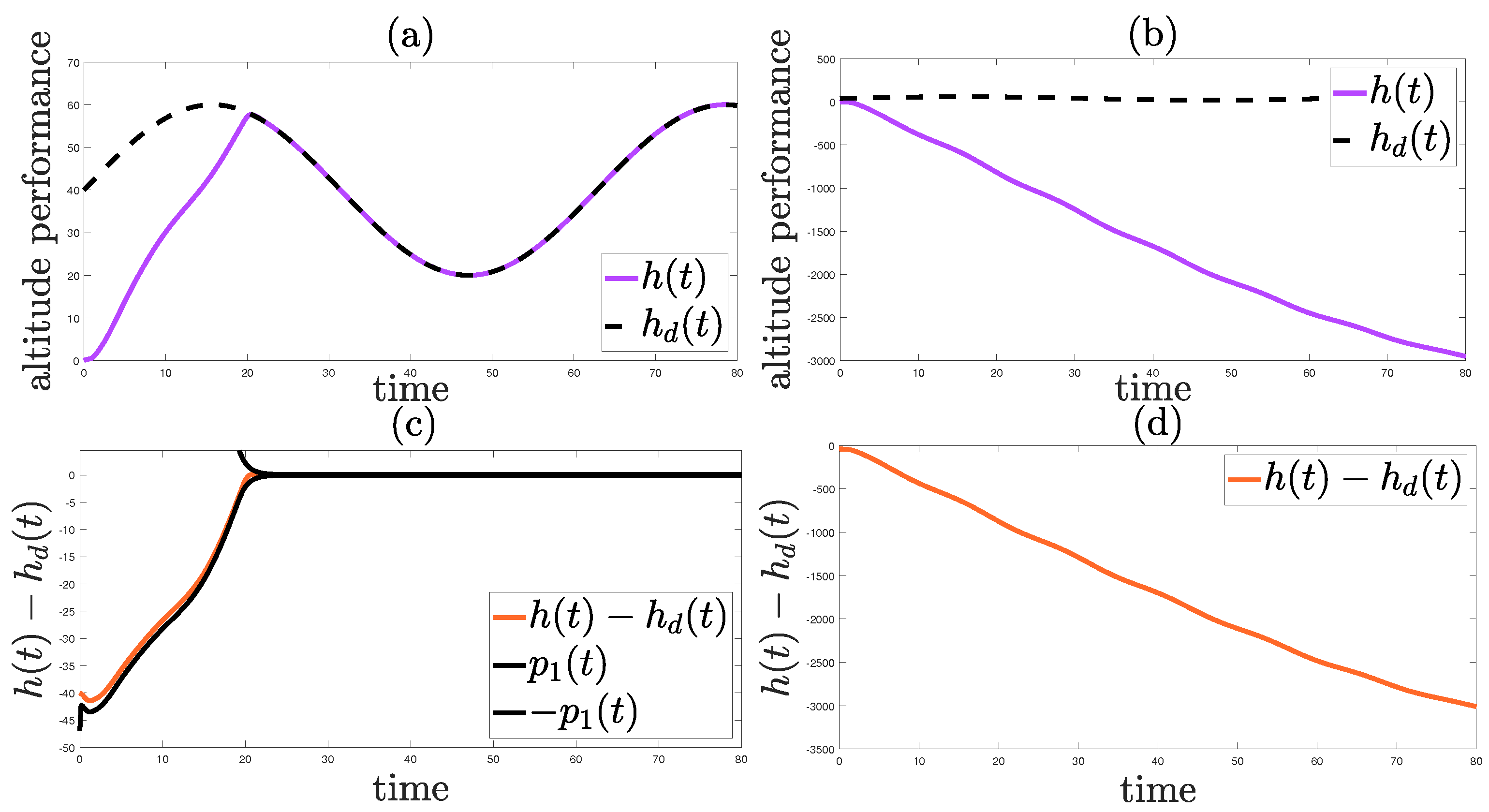
• The desired trajectory $y_d:={[h_d\left(t\right),V_d\left(t\right)]}^T$ is tracked with adaptive prescribed performance specifications.

Finally, to solve the aforementioned problem, we pose the following assumptions:

Assumption 1.

The state of the system x is considered available for measurement.

Assumption 2.

The desired trajectory $y_d$ as well as the signal ${\dot{h}}_d\left(t\right)$ are known bounded functions of time.

Assumption 3.

The external disturbances $d\left(t\right)$ are unknown bounded and piecewise continuous functions of time.

Preliminaries on PPC

In the PPC framework, the focus is on achieving a specific behavior in terms of the output tracking error performance. This involves ensuring that the error converges to a predetermined residual set with a predefined minimum convergence rate. In the context of the approximation-free approach proposed in [29], the tracking error $e\left(t\right)$ is defined as the difference between the measured output $y\left(t\right)$ and the desired reference trajectory $y_d\left(t\right)$. To quantify the desired performance, a performance function $p\left(t\right)$ is chosen, which is expressed as a decaying exponential function with parameters $p\left(0\right)$, $p_{\infty }$, and $\lambda$. In particular, $p_{\infty }$ represents the maximum allowable absolute error at steady state and $\lambda$ determines the rate of convergence. Thus, the prescribed performance requirement is met if the tracking error $e\left(t\right)$ remains within the performance envelope defined by performance functions $p\left(t\right)$ and $-p\left(t\right)$, respectively, for all $t\ge 0$ (i.e., $-p\left(t\right)<e\left(t\right)<p\left(t\right),\forall t\ge 0$). Finally, it is important to note that the initial tracking error $e\left(0\right)$ should be accounted for in the performance envelope, satisfying the condition $p\left(0\right)>\left|e\right(0\left)\right|$ at $t=0$.

3. Controller Design

In this section, we present an APPC control scheme for trajectory tracking of state and input constrained UAVs with longitudinal dynamics given by (7). Let us first define the error transformation function $\mathcal{T}\left(\chi \right)=\frac{1}{2}\ln \left(\frac{1+\chi }{1-\chi }\right)$ as well as its Jacobian $\mathcal{D}\left(\chi \right)=\frac{1}{1-{\chi }^2}$. The system constraints are incorporated by a differentiable saturation function $\sigma (·,\overline{\sigma }):\mathbb{R}\to [-\overline{\sigma },\overline{\sigma }]$, where $\overline{\sigma }>0$ corresponds to the saturation level. In this work, we adopt the following saturation function:

$$\begin{array}{c}\hfill \sigma (\chi ,\overline{\sigma })=\left\{\begin{array}{cc}\chi \hfill & \mathrm{if}\left|\chi \right|<\overline{\sigma }-\beta \hfill \\ p\left(\chi \right)\hfill & \mathrm{if}\left|\chi \right|\in [\overline{\sigma }-\beta ,\overline{\sigma }+\beta ]\hfill \\ s_{\chi }\overline{\sigma }\hfill & \mathrm{if}\left|\chi \right|>\overline{\sigma }+\beta \hfill \end{array}\right.\end{array}$$

where:

$$p\left(\chi \right)=-\frac{1}{4\beta }\left({\chi }^2-2s_{\chi }(\overline{\sigma }+\beta )\chi +{(s_{\chi }\overline{\sigma }-s_{\chi }\beta )}^2\right)$$

with $s_{\chi }$ denoting the $\mathrm{sign}$ of $\chi$ and $\beta ={10}^{-6}$ is a small smoothing parameter. The input constraints are then determined directly by elevator deflection ${\overline{\delta }}_e$ as well as the throttle amplitude and rate saturation levels ${\overline{\delta }}_T,\overline{r}$, respectively. The state constraints are regulated indirectly. First, the generated reference state trajectories ${\gamma }_d\left(t\right),{\theta }_d\left(t\right),q_d\left(t\right)$ are saturated according to the saturation levels $\overline{\gamma },\overline{\theta },\overline{q}$, respectively. Then by employing the APPC approach we impose state constraints depending both on the corresponding reference constraints and the adaptive performance specifications. The design procedure of the proposed controller is described as follows:

Step 1. In order to design the desired flight-path-angle ${\gamma }_d\left(t\right)$ for a reference trajectory $y_d\left(t\right)$ we exploit (1) in combination with the PPC technique. In particular, we create the closed-loop altitude dynamics as:

$${\dot{h}}_d\left(t\right)=V_d\left(t\right)sin{\gamma }_d\left(t\right)+k_h\mathcal{D}\left(\frac{h\left(t\right)-h_d\left(t\right)}{p_1\left(t\right)}\right)\mathcal{T}\left(\frac{h\left(t\right)-h_d\left(t\right)}{p_1\left(t\right)}\right)$$

where $p_1\left(t\right)$ is an adaptive performance function (PF) to be designed, $k_h$ is a control gain, and ${\gamma }_d$ is the reference flight-path-angle. Given that the reference flight-path-angle should be constrained within a small set of angles, we obtain the desired constrained flight-path-angle trajectory as:

$${\gamma }_d\left(t\right)=arcsin\left(\sigma \left(\frac{-\eta \left(t\right)}{V_d\left(t\right)},sin\left(\overline{\gamma }\right)\right)\right).$$

(8)

where $\eta :=k_h\mathcal{D}\left(\frac{h\left(t\right)-h_d\left(t\right)}{p_1\left(t\right)}\right)\mathcal{T}\left(\frac{h\left(t\right)-h_d\left(t\right)}{p_1\left(t\right)}\right)-{\dot{h}}_d\left(t\right)$. Next design the adaptive performance function that incorporates the output performance specifications and the reference signal constraints:

$$\begin{array}{cc}\hfill {\dot{p}}_1\left(t\right)& =-{\lambda }_h(p_1\left(t\right)-p_{\infty }^1)+\eta \left(t\right)\left(sin{\gamma }_d\left(t\right)+\frac{\eta \left(t\right)}{V_d\left(t\right)}\right)\hfill \end{array}$$

(9)

where ${\lambda }_h,p_{\infty }^1>0$ regulate the desired minimum exponential convergence rate and the maximum absolute value of steady state altitude error, respectively. Note that the saturation level $\overline{\gamma }$ directly affects the performance specifications of the altitude tracking error as small angles $\gamma$ do not allow fast variation in the UAV’s altitude. In particular, the first term of (9) stands for the conventional strictly decreasing term $(p_1\left(0\right)-p_{\infty }^1)exp(-{\lambda }_{h}t)+p_{\infty }^1$, whereas the second term, which is non-negative, relaxes the performance specifications by increasing $p_1\left(t\right)$, in order to maintain the altitude tracking error within an adaptive performance funnel, which guarantees the boundedness of the transformed error $\mathcal{T}\left(\frac{h\left(t\right)-h_d\left(t\right)}{p_1\left(t\right)}\right)$. Notice also that $sin{\gamma }_d\left(t\right)=sin{\gamma }_u\left(t\right)$ when the saturation is not active. Thus, the relaxed performance function recovers its conventional form with exponential decay rate when the system operates without saturation.

Step 2. Next, select the reference force vector along with the corresponding performance update laws as:

$$\begin{array}{cc}\hfill F_x\left(t\right)& =-\frac{k_v}{p_2\left(t\right)}\mathcal{D}\left(\frac{V\left(t\right)-V_d\left(t\right)}{p_2\left(t\right)}\right)\mathcal{T}\left(\frac{V\left(t\right)-V_d\left(t\right)}{p_2\left(t\right)}\right)\hfill \end{array}$$

(10)

$$\begin{array}{cc}\hfill {\dot{p}}_2\left(t\right)& =-{\lambda }_v(p_2\left(t\right)-p_{\infty }^2)+\frac{V\left(t\right)-V_d\left(t\right)}{p_2\left(t\right)}\left(\sigma (F_x\left(t\right),|{\overline{\delta }}_{T}cosa\left(t\right)\left|\right)-F_x\left(t\right)\right)\hfill \end{array}$$

(11)

$$\begin{array}{cc}\hfill F_h\left(t\right)& =-\frac{k_{\gamma }}{V\left(t\right)p_3\left(t\right)}\mathcal{D}\left(\frac{\gamma \left(t\right)-{\gamma }_d\left(t\right)}{p_3\left(t\right)}\right)\mathcal{T}\left(\frac{\gamma \left(t\right)-{\gamma }_d\left(t\right)}{p_3\left(t\right)}\right)\hfill \end{array}$$

(12)

$$\begin{array}{cc}\hfill {\dot{p}}_3\left(t\right)& =-{\lambda }_{\gamma }(p_3\left(t\right)-p_{\infty }^3)+\frac{\gamma \left(t\right)-{\gamma }_d\left(t\right)}{p_3\left(t\right)}\left(\sigma (F_h\left(t\right),|{\overline{\delta }}_{T}sina\left(t\right)\left|\right)-F_h\left(t\right)\right).\hfill \end{array}$$

(13)

with $k_v,k_{\gamma },{\lambda }_v,{\lambda }_{\gamma },p_{\infty }^2,p_{\infty }^3>0$. Notice that $F_x\left(t\right),F_h\left(t\right)$ act as controls in (2) and (3), regulating the horizontal and vertical motion of the system, respectively. Thus, the reference unconstrained throttle command as well as the corresponding angle-of-attack are given by $u_d:=\sqrt{F_x{\left(t\right)}^2+F_h{\left(t\right)}^2}$ and $a_d:=arctan\left(\frac{F_h\left(t\right)}{F_x\left(t\right)}\right)$, respectively. The saturation levels incorporated into the adaptive PFs (11) and (13) take into account the feasible generated thrust depending on the actual angle-of-attack. In order to impose both input and rate constraints to the control input ${\delta }_T\left(t\right)$ we utilize the APPC technique developed in [32] which leads us to:

$$\begin{array}{cc}\hfill {\tilde{\delta }}_T\left(t\right)& =-k_r\mathcal{D}\left(\frac{{\delta }_T\left(t\right)-\sigma (u_d\left(t\right),{\overline{\delta }}_T)}{p_4\left(t\right)}\right)\mathcal{T}\left(\frac{{\delta }_T\left(t\right)-\sigma (u_d\left(t\right),{\overline{\delta }}_T)}{p_4\left(t\right)}\right)\hfill \end{array}$$

(14)

$$\begin{array}{cc}\hfill {\dot{p}}_4\left(t\right)& =-{\lambda }_r(p_4\left(t\right)-p_{\infty }^4)+\frac{{\delta }_T\left(t\right)-\sigma (u_d\left(t\right),{\overline{\delta }}_T)}{p_4\left(t\right)}\left(\sigma ({\tilde{\delta }}_T\left(t\right),\overline{r})-{\tilde{\delta }}_T\left(t\right)\right)\hfill \end{array}$$

(15)

with $k_r,{\lambda }_r,p_{\infty }^4>0$, where the input amplitude and rate limitations are regulated by ${\overline{\delta }}_T$ and $\overline{r}$, respectively. The dynamic throttle command is then obtained by:

$${\dot{\delta }}_T:=\varphi \left(t\right)=\sigma ({\tilde{\delta }}_T\left(t\right),\overline{r}).$$

(16)

Step 3. Subsequently, consider the constrained pitch reference trajectory:

$${\theta }_d\left(t\right)=\sigma (a_d\left(t\right)+{\gamma }_d\left(t\right),\overline{\theta })$$

(17)

where $\overline{\theta }$ denotes the maximum absolute value of the reference pitch angle. Moreover, as ${\gamma }_d\left(t\right)$ is also constrained within the compact set $[-\overline{\gamma },\overline{\gamma }]$, the reference angle-of-attack $a_d\left(t\right)$ lies within the set $[-\overline{\theta }+\overline{\gamma },\overline{\theta }-\overline{\gamma }]$. Finally, utilizing once again the APPC technique we obtain the constrained elevator control command as:

$$\begin{array}{cc}\hfill q_d\left(t\right)& =-k_{\theta }\mathcal{D}\left(\frac{\theta \left(t\right)-{\theta }_d\left(t\right)}{p_5\left(t\right)}\right)\mathcal{T}\left(\frac{\theta \left(t\right)-{\theta }_d\left(t\right)}{p_5\left(t\right)}\right)\hfill \end{array}$$

(18)

$$\begin{array}{cc}\hfill {\dot{p}}_5\left(t\right)& =-{\lambda }_{\theta }(p_5\left(t\right)-p_{\infty }^5)+\frac{\theta \left(t\right)-{\theta }_d\left(t\right)}{p_5\left(t\right)}\left(\sigma (q_d\left(t\right),\overline{\theta })-q_d\left(t\right)\right)\hfill \end{array}$$

(19)

$$\begin{array}{cc}\hfill {\tilde{\delta }}_e\left(t\right)& =k_q\mathcal{D}\left(\frac{q\left(t\right)-\sigma (q_d\left(t\right),\overline{q})}{p_6\left(t\right)}\right)\mathcal{T}\left(\frac{q\left(t\right)-\sigma (q_d\left(t\right),\overline{q})}{p_6\left(t\right)}\right)\hfill \end{array}$$

(20)

$$\begin{array}{cc}\hfill {\dot{p}}_6\left(t\right)& =-{\lambda }_q(p_6\left(t\right)-p_{\infty }^6)-\frac{q\left(t\right)-\sigma (q_d\left(t\right),\overline{q})}{p_6\left(t\right)}\left(\sigma ({\tilde{\delta }}_e\left(t\right),{\overline{\delta }}_e)-{\tilde{\delta }}_e\left(t\right)\right)\hfill \end{array}$$

(21)

with $k_{\theta },k_q,{\lambda }_{\theta },{\lambda }_q,p_{\infty }^5,p_{\infty }^6>0$. Finally the constrained elevator deflection applied to the UAV is:

$${\delta }_e:=\sigma ({\tilde{\delta }}_e\left(t\right),{\overline{\delta }}_e).$$

(22)

According to [33], it is customary to assign a positive sign to the elevator control signal ${\tilde{\delta }}_e\left(t\right)$, representing the primary deflection of the elevator. The function $M(a,V,{\delta }_e,q)$ exhibits strictly decreasing behavior and thus, a positive deflection of the elevator generates a nose-down pitching moment, while a negative deflection elicits a nose-up pitching moment. The proposed control scheme (8)–(22) is summarized in

Table 1. Control Scheme.

Intermediate Commands
${\gamma }_d\left(t\right)=arcsin\left(\sigma \left(\frac{-\eta \left(t\right)}{V_d\left(t\right)},sin\left(\overline{\gamma }\right)\right)\right)$ see (8)
$F_x\left(t\right)=-\frac{k_v}{p_2\left(t\right)}\mathcal{D}\left(\frac{V\left(t\right)-V_d\left(t\right)}{p_2\left(t\right)}\right)\mathcal{T}\left(\frac{V\left(t\right)-V_d\left(t\right)}{p_2\left(t\right)}\right)$ see (10)
$F_h\left(t\right)=-\frac{k_{\gamma }}{V\left(t\right)p_3\left(t\right)}\mathcal{D}\left(\frac{\gamma \left(t\right)-{\gamma }_d\left(t\right)}{p_3\left(t\right)}\right)\mathcal{T}\left(\frac{\gamma \left(t\right)-{\gamma }_d\left(t\right)}{p_3\left(t\right)}\right)$ see (12)
$u_d\left(t\right)=\sqrt{F_x{\left(t\right)}^2+F_h{\left(t\right)}^2}$
$a_d\left(t\right)=arctan\left(\frac{F_h\left(t\right)}{F_x\left(t\right)}\right)$
${\tilde{\delta }}_T\left(t\right)=-k_r\mathcal{D}\left(\frac{{\delta }_T\left(t\right)-\sigma (u_d\left(t\right),{\overline{\delta }}_T)}{p_4\left(t\right)}\right)\mathcal{T}\left(\frac{{\delta }_T\left(t\right)-\sigma (u_d\left(t\right),{\overline{\delta }}_T)}{p_4\left(t\right)}\right)$ see (14)
${\theta }_d\left(t\right)=\sigma (a_d\left(t\right)+{\gamma }_d\left(t\right),\overline{\theta })$ see (17)
$q_d\left(t\right)=-k_{\theta }\mathcal{D}\left(\frac{\theta \left(t\right)-{\theta }_d\left(t\right)}{p_5\left(t\right)}\right)\mathcal{T}\left(\frac{\theta \left(t\right)-{\theta }_d\left(t\right)}{p_5\left(t\right)}\right)$ see (18)
${\tilde{\delta }}_e\left(t\right)=k_q\mathcal{D}\left(\frac{q\left(t\right)-\sigma (q_d\left(t\right),\overline{q})}{p_6\left(t\right)}\right)\mathcal{T}\left(\frac{q\left(t\right)-\sigma (q_d\left(t\right),\overline{q})}{p_6\left(t\right)}\right)$ see (20)
Adaptive performance functions
${\dot{p}}_1\left(t\right)=-{\lambda }_h(p_1\left(t\right)-p_{\infty }^1)+\eta \left(t\right)\left(sin{\gamma }_d\left(t\right)+\frac{\eta \left(t\right)}{V_d\left(t\right)}\right)$ see (9)
${\dot{p}}_2\left(t\right)=-{\lambda }_v(p_2\left(t\right)-p_{\infty }^2)+\frac{V\left(t\right)-V_d\left(t\right)}{p_2\left(t\right)}\left(\sigma (F_x\left(t\right),|{\overline{\delta }}_{T}cosa\left(t\right)\left|\right)-F_x\left(t\right)\right)$ see (11)
${\dot{p}}_3\left(t\right)=-{\lambda }_{\gamma }(p_3\left(t\right)-p_{\infty }^3)+\frac{\gamma \left(t\right)-{\gamma }_d\left(t\right)}{p_3\left(t\right)}\left(\sigma (F_h\left(t\right),|{\overline{\delta }}_{T}sina\left(t\right)\left|\right)-F_h\left(t\right)\right)$ see (13)
${\dot{p}}_4\left(t\right)=-{\lambda }_r(p_4\left(t\right)-p_{\infty }^4)+\frac{{\delta }_T\left(t\right)-\sigma (u_d\left(t\right),{\overline{\delta }}_T)}{p_4\left(t\right)}\left(\sigma ({\tilde{\delta }}_T\left(t\right),\overline{r})-{\tilde{\delta }}_T\left(t\right)\right)$ see (15)
${\dot{p}}_5\left(t\right)=-{\lambda }_{\theta }(p_5\left(t\right)-p_{\infty }^5)+\frac{\theta \left(t\right)-{\theta }_d\left(t\right)}{p_5\left(t\right)}\left(\sigma (q_d\left(t\right),\overline{\theta })-q_d\left(t\right)\right)$ see (19)
${\dot{p}}_6\left(t\right)=-{\lambda }_q(p_6\left(t\right)-p_{\infty }^6)-\frac{q\left(t\right)-\sigma (q_d\left(t\right),\overline{q})}{p_6\left(t\right)}\left(\sigma ({\tilde{\delta }}_e\left(t\right),{\overline{\delta }}_e)-{\tilde{\delta }}_e\left(t\right)\right)$ see (21)
Control inputs
${\dot{\delta }}_T\left(t\right)=\sigma ({\tilde{\delta }}_T\left(t\right),\overline{r})$ see (16)
${\delta }_e\left(t\right)=\sigma ({\tilde{\delta }}_e\left(t\right),{\overline{\delta }}_e)$ see (22)

for readers’ convenience.

Theorem 1.

Consider system (7), an output reference trajectory $y_d\left(t\right)$ that obeys Assumptions 1–3 and the constrained reference state vector $r_d:={[{\gamma }_d\left(t\right),{\theta }_d\left(t\right),q_d\left(t\right)]}^T$ generated by (8)–(22). For sufficiently large saturation levels ${\overline{\delta }}_T,{\overline{\delta }}_e$, there exist upper bounds ${\overline{p}}_i,i=1,\cdots ,6$ of the performance function $p_i\left(t\right)$ such that the proposed adaptive control scheme (8)–(22) guarantees:

$$\begin{array}{cc}\hfill \parallel x_i\left(t\right)-x_{d_i}\left(t\right)\parallel & <p_i\left(t\right)<{\overline{p}}_i,i=1,\cdots ,6\hfill \end{array}$$

for all $t\ge 0$ with $x_d:={[y_d^T,r_d^T]}^T$.

Proof .

Let us first define the normalized tracking error vector:

$$\begin{array}{c}\hfill \xi :=\left[\begin{array}{c}\frac{h\left(t\right)-h_d\left(t\right)}{p_1\left(t\right)}\\ \frac{V\left(t\right)-V_d\left(t\right)}{p_2\left(t\right)}\\ \frac{\gamma \left(t\right)-{\gamma }_d\left(t\right)}{p_3\left(t\right)}\\ \frac{{\delta }_T\left(t\right)-\sigma (u_d\left(t\right),{\overline{\delta }}_T)}{p_4\left(t\right)}\\ \frac{\theta \left(t\right)-{\theta }_d\left(t\right)}{p_5\left(t\right)}\\ \frac{q\left(t\right)-\sigma (q_d\left(t\right),\overline{q})}{p_6\left(t\right)}\end{array}\right]\end{array}$$

(23)

Differentiating $\xi \left(t\right)$ with respect to time we obtain the augmented closed-loop dynamical system as:

$$\begin{array}{c}\hfill \dot{\zeta }:={[\dot{\xi }{\left(t\right)}^T,{\dot{p}}_1\left(t\right),{\dot{p}}_2\left(t\right),{\dot{p}}_3\left(t\right),{\dot{p}}_4\left(t\right),{\dot{p}}_5\left(t\right),{\dot{p}}_6\left(t\right)]}^T.\end{array}$$

(24)

Next, let us define the open set:

$$\mathsf{\Omega }:=\stackrel{6\mathrm{times}}{\overbrace{(-1,1)\times ...\times (-1,1)}}\times (0,\overline{p_1})\times ...\times (0,\overline{p_6})\subset {\mathbb{R}}^{12}.$$

Then, the proof proceeds in three phases. First the existence of a unique maximal solution $\zeta :[0,{\tau }_{max})\to \mathsf{\Omega }$ of (24) is ensured, i.e., $\zeta \left(t\right)\in \mathsf{\Omega },\forall t\in [0,{\tau }_{max})$. Next, we establish a sufficient condition regarding the saturation levels, such that the proposed control scheme guarantees the boundedness of all closed-loop signals of (24) for all $t\in [0,{\tau }_{\infty })$. Finally, we prove that $\zeta$ remains strictly within a compact subset of $\mathsf{\Omega }$, which leads to ${\tau }_{max}=\infty$ by contradiction.

Phase A. Consider the closed-loop dynamical system (24). By construction, it holds that $\left|{\xi }_i\left(0\right)\right|<1,p_i\left(0\right)\in (0,{\overline{p}}_i),i=1,\cdots ,6$ and therefore $\zeta \left(0\right)\in \mathsf{\Omega }$. Moreover, $\dot{\zeta }:\mathsf{\Omega }\to {\mathbb{R}}^{12}$ is piece-wise continuous and locally integratable on t as well as locally $\mathrm{Lipschitz}$ on $\zeta$, over the open set $\mathsf{\Omega }$. Hence, invoking Theorem 54 in [34] (p. 476) we conclude that there exists a unique maximal solution $\zeta :[0,{\tau }_{max})\to \mathsf{\Omega },\forall t\in [0,{\tau }_{max})$.

Phase B.

In Phase A, we showed that $\zeta \left(t\right)\in \mathsf{\Omega },\forall t\in [0,{\tau }_{max})$, which implies that the transformed errors ${ϵ}_i:=\mathcal{T}\left({\xi }_i\left(t\right)\right),i=1,\cdots ,6$ are well defined for all $t\in [0,{\tau }_{max})$ since ${\xi }_i\left(t\right)\in (-1,1),i=1,\cdots ,6$. The Phase B of this proof is divided into three parts, where a sufficient boundedness condition, for the signals ${ϵ}_i\left(t\right),p_i\left(t\right),i=1,\cdots ,n$ is provided in each part.

Phase B.1 First consider the positive definite and radially unbounded $\mathrm{Lyapunov}$ function candidate $V_1=\frac{1}{2}{ϵ}_1^2\left(t\right)$. By differentiating $V_1$ with respect to time, we obtain:

$$\begin{array}{cc}\hfill {\dot{V}}_1=& \frac{{ϵ}_1\left(t\right)}{(1-{\xi }_1^2\left(t\right))p_1\left(t\right)}(\dot{h}\left(t\right)-{\dot{h}}_d\left(t\right)-{\xi }_1\left(t\right){\dot{p}}_1\left(t\right)).\hfill \end{array}$$

(25)

Substituting (1) and (8)–(9) we obtain:

$$\begin{array}{cc}\hfill {\dot{V}}_1=& \frac{{ϵ}_1\left(t\right)}{(1-{\xi }_1^2\left(t\right))p_1\left(t\right)}(V\left(t\right)sin\gamma \left(t\right)+w_h\left(t\right)-{\dot{h}}_d\left(t\right)\hfill \\ & +{\xi }_1\left(t\right){\lambda }_h(p_1\left(t\right)-p_{\infty }^1)-{\xi }_1\left(t\right)\eta \left(t\right)\left(sin\left({\gamma }_d\left(t\right)\right)+\frac{\eta \left(t\right)}{V_d\left(t\right)}\right)).\hfill \end{array}$$

(26)

Next owing to the continuity of the unknown dynamics of (7) and exploiting Assumptions 2 and 3 we obtain:

$${\overline{F}}_1:=\underset{\zeta \in \mathsf{\Omega }}{max}\left\{\left|V\left(t\right)sin\gamma \left(t\right)+w_h\left(t\right)-{\dot{h}}_d\left(t\right)+{\xi }_1\left(t\right){\lambda }_h(p_1\left(t\right)-p_{\infty }^1)\right|\right\}.$$

Additionally, $\frac{1}{(1-{\xi }_1^2\left(t\right))}>1$ as ${\xi }_1\left(t\right)\in (-1,1),\forall t\in [0,{\tau }_{max})$, whereas $p_1\left(t\right)\ge p_{1,\infty }>0$ by construction. Thus, owing to the last term of (26) we conclude that there exists a function $w(·)\in {\mathcal{K}}_{\infty }$ such that:

$$\begin{array}{cc}\hfill {\dot{V}}_1\le & \frac{1}{(1-{\xi }_1^2\left(t\right))p_1\left(t\right)}\left(-w\left(\right|{ϵ}_1\left(t\right)\left|\right)|{ϵ}_1\left(t\right)|+{\overline{F}}_1\left|{ϵ}_1\left(t\right)\right|\right).\hfill \end{array}$$

(27)

Therefore, ${\dot{V}}_1$ becomes negative when $ϵ\left(t\right)>{\overline{ϵ}}_1$ for some positive constant ${\overline{ϵ}}_1$ such that $w\left({\overline{ϵ}}_1\right)={\overline{F}}_1$, leading to ultimately boundedness of ${ϵ}_1\left(t\right)$ with respect to a compact set:

$${\mathcal{E}}_1:=\left\{{ϵ}_1:\left|{ϵ}_1\left(t\right)\right|\le \underset{\zeta \in \mathsf{\Omega }}{max}\left\{\left|{ϵ}_1\left(0\right)\right|,{\overline{ϵ}}_1\right\}\right\}.$$

(28)

Note that the existence of a performance bound ${\overline{p}}_1$ at a time instant $t=t_p$, such that the right hand side of (9) becomes negative when $p_1\left(t\right)={\overline{p}}_1$ and $\left|{ϵ}_1\left(t\right)\right|={ϵ}_{1,\overline{p}}<{\overline{ϵ}}_1$, implies the existence of a small positive constant ${\delta }_1$ such that $p_1\left(t\right)\in [p_{\infty }^1,{\overline{p}}_1-{\delta }_1],\forall t\in [0,{\tau }_{max})$. Specifically, utilizing (9), we conclude that $p_1\left(t\right)\in {\mathsf{\Omega }}_{p_1}$, with:

$${\mathsf{\Omega }}_{p_1}:=[p_{\infty }^1,{\overline{p}}_1-{\delta }_1]$$

(29)

when the saturation level $\overline{\gamma }$ satisfies the following inequality:

$$\overline{\gamma }>-\frac{{\lambda }_1({\overline{p}}_1-p_{\infty }^1)-\frac{{\eta }^2\left(t_p\right)}{V_d\left(t_p\right)}}{\mathrm{sign}\left(\eta \left(t_p\right)\right)\eta \left(t_p\right)}.$$

(30)

Phase B.2–3 Regarding the boundedness of ${ϵ}_i\left(t\right),p_i\left(t\right),i=2,3,4$, Phase B.2, consider the Lyapunov function candidate $V_2=\frac{1}{2}{ϵ}_2^2+\frac{1}{2}{ϵ}_3^2$ (as in [30]) and $V_4=\frac{1}{2}{ϵ}_4^2$ as well as (Phase B.3) the functions $V_i=\frac{1}{2}{ϵ}_i^2,i=5,\cdots ,6$ in order to prove the boundedness of ${ϵ}_i\left(t\right),p_i\left(t\right),i=4,5$, respectively. Subsequently, it is easy to obtain stability sets ${\mathcal{E}}_i,{\mathsf{\Omega }}_{p_i},i=2,\cdots ,6$ for ${ϵ}_i\left(t\right),p_i\left(t\right),i=2,\cdots ,6$ similar to (28) and (29), by following the analysis presented in [32] with minor modifications.

Phase C. In Phase B, we proved the boundedness of the transformed errors ${ϵ}_i\left(t\right)=\mathcal{T}\left({\xi }_i\left(t\right)\right),i=1,\cdots ,6$ for all $t\in [0,{\tau }_{max})$ within the compact sets ${\mathcal{E}}_{i}i=1,\cdots ,6$ for sufficiently large saturation levels. Utilizing this with the inverse of function $\mathcal{T}$, we conclude the boundedness of the normalized errors ${\xi }_i\left(t\right)i=1,\cdots ,6$ within the compact sets ${\mathsf{\Omega }}_{{\xi }_i}:=[{\underline{\xi }}_i,{\overline{\xi }}_i]\subset (-1,1),i=1,\cdots ,6$. Moreover we showed that the adaptive performance functions $p_i\left(t\right)\in {\mathsf{\Omega }}_{p_i}\subset (0,{\overline{p}}_i),i=1,\cdots ,6$. Note that $\zeta \left(t\right)\in {\mathsf{\Omega }}^{\prime }\subset \mathsf{\Omega },\forall t\in [0,{\tau }_{max})$, with ${\mathsf{\Omega }}^{\prime }:={\mathsf{\Omega }}_{{\xi }_i}\times {\mathsf{\Omega }}_{p_i},i=1,\cdots ,6$. Thus, assuming that ${\tau }_{max}<\infty$, then according to Proposition C.3.6 in [34] (p. 481) there exists a time instant ${\tau }^{\prime }$ such that $\zeta \left({\tau }^{\prime }\right)\notin {\mathsf{\Omega }}^{\prime }$, which is a contradiction. As a consequence, ${\tau }_{max}=\infty$, which implies the stability of the initial system (7). Finally, invoking the fact that ${\xi }_i\left(t\right)\in {\mathsf{\Omega }}_{{\xi }_i},i=1,\cdots ,6$ for all $t\ge 0$ we conclude that:

$$\parallel x_i\left(t\right)-x_{d_i}\left(t\right)\parallel <p_i\left(t\right)<{\overline{p}}_i$$

for all $t\ge 0$ and $i=1,\cdots ,6$ with $x_d:={[h_d\left(t\right),V_d\left(t\right),{\gamma }_d\left(t\right),\sigma (u_d\left(t\right),{\overline{\delta }}_T),{\theta }_d\left(t\right),\sigma (q_d\left(t\right),\overline{q})]}^T$. Note that both the state and output errors evolve strictly within the adaptive performance envelope, which completes the proof. □

Remark 1.

Note that the constraint regarding the elevator deflection ${\delta }_e\left(t\right)$ is imposed directly by saturating the control signal (20), whereas the throttle limit is achieved by exploiting two nested saturation constraints in combination with the APPC approach that guarantees $\parallel {\delta }_T\left(t\right)\parallel \le {\overline{\delta }}_T$ and $\parallel {\dot{\delta }}_T\left(t\right)\parallel \le r$. Furthermore, state constraints on $\gamma \left(t\right),\theta \left(t\right),q\left(t\right)$ are guaranteed via saturating the reference state trajectories ${\gamma }_d\left(t\right),{\theta }_d\left(t\right),q_d\left(t\right)$, while imposing tracking with adaptive prescribed transient and steady-state specifications. Thus, the system will operate in a compact set $\mathcal{X}$, the size of which is determined by the desired state constraints, i.e., the saturation levels of the state reference trajectories in combination with the adaptive performance specifications affected by input limitations and the couplings among system dynamics.

Remark 2.

The proposed control scheme (8)–(22) does not require either knowledge of the system nonlinearities or any approximating structures exhibiting robustness against unknown external disturbances. Additionally, both the intermediate control signals and the adaptive performance functions are obtained through simple calculations preventing the explosion of complexity. Finally, the simple gain selection facilitates the practical application of the proposed algorithm.

Remark 3.

The appropriate saturation level $\overline{\sigma }$ of the control signals and the states that prevents the finite-time blow-up of the closed-loop system is affected by various factors. Such factors include the unknown system dynamics and external disturbances as well as the strong couplings among the states of the system and the reference trajectory. For example, small control inputs, i.e., small input saturation levels, may be insufficient to prevent the system from becoming unstable in case of large airspeed and wind gusts. Hence, the proper selection of saturation levels in accordance to the reference trajectory constitutes a pivotal task so that the stability of the closed-loop system is ensured.

4. Comprehensive Simulation on UAV Landing Scenario

In this section, we demonstrate the effectiveness of the proposed controller by conducting a simulation study using an Aerosonde UAV, as described in [33]. The objective is to guide the UAV in tracking a predetermined reference trajectory for landing, while accounting wind disturbances, predefined input constraints as well as adaptive prescribed performance output and state constraints. The aerodynamic longitudinal coefficients of the Aerosonde model are presented in

Table 2. Aerodynamic coefficients.

Parameter	Value	Longitudinal Coefficient	Value
m	13.5 kg	$C_{L_0}$	$0.28$
$I_{yy}$	1.135 kg m ${}^2$	$C_{L_a}$	$3.45$
S	0.55 m${}^2$	$C_{L_{{\delta }_e}}$	$-0.36$
$\overline{c}$	0.18994 m	$C_{D_0}$	$0.03$
$C_{prop}$	1 m${}^2$	$C_{D_a}$	$0.3$
$S_{prop}$	0.2027 m${}^2$	$C_{M_0}$	$-0.02338$
$\rho$	1.2682 kg/m${}^3$	$C_{M_a}$	$-0.38$
$k_m$	80	$C_{M_q}$	$-3.6$
g	$9.8$	$C_{M_{{\delta }_e}}$	$-0.5$

, whereas the parameters of the control scheme are outlined in

Table 3. Control Scheme parameters.

Parameter	Value
$k_i,i\in \{h,v,\gamma ,\theta ,q,r\}$	2
${\lambda }_i,i\in \{h,v,\gamma ,\theta ,q\}$	$0.5$
${\lambda }_r$	20
$p_{\infty }^i,i\in \{1,2,4\}$	$0.05$
$p_{\infty }^i,i\in \{3,5,6\}$	$0.005$
${\overline{\delta }}_T$	$0.65$
$\overline{r}$	$0.25$
${\overline{\delta }}_e\left(rad\right)$	$0.2$
$\overline{\gamma }\left(rad\right)$	$0.06$
$\overline{\theta }\left(rad\right)$	$0.1$
$\overline{q}\left(rad\right)$	$0.1$

. It is worth noting that the throttle settling limit is intentionally set at $65\%$ to showcase the proposed controller’s ability to handle performance specifications alongside input limitations. Moreover, Remark 2 emphasizes that the task of selecting the gains is straightforward, hence all control gains $k_i$ are uniformly set to validate this claim. The reference landing trajectory is defined as $h_d\left(t\right)=100\frac{exp(-0.07t)-1}{exp(-0.07(t-100\left)\right)+1}+100$ and the airspeed profile is chosen as $V_d\left(t\right)=50-5sin\left(0.0038t\right)$. Furthermore the initial state conditions are selected as $x\left(0\right)={[95,45,0.04,0.03,0,0]}^T$ and the initial values of the adaptive performance functions are set to $p_1\left(0\right)=6.75,p_2\left(0\right)=5.5,p_3\left(0\right)=0.12,p_4\left(0\right)=0.13,p_5\left(0\right)=0.2,p_6\left(0\right)=1.65$. Finally, in order to demonstrate the robustness of the proposed control scheme, we induce wind gusts $w_x\left(t\right)=1.5sin\left(0.0335t\right),w_h\left(t\right)=2cos\left(0.05t\right),\forall t\in [10,104.25]$ for a simulation period of 200 s.

The adaptive prescribed performance of the altitude tracking error is depicted in Figure 2a, where the proposed PFs create an adaptive performance envelope within which the tracking error is evolving. Note that the conventional PFs are denoted by dotted-lines and as one can see the performance specifications are relaxed at the time instant the wind starts affecting the dynamics of the system, in order to maintain the altitude tracking error strictly inside the performance envelope when the output constraints are conflicting with the input and state saturation, i.e., the altitude variation rate is delimited by the saturated control effort applied by the actuators. The latter is also affected by the maximum absolute value of flight-path angle, angle-of-attack and pitch rate that are imposed by our control scheme, in order to ensure the safety of landing procedure. Additionally, the performance of UAV’s altitude versus the reference landing trajectory is depicted in Figure 2b.

Similar results regarding the tracking performance of the airspeed trajectory are shown in Figure 3. Notice that the excessive relaxation of the performance envelope during the transient period is owing to the heavily saturated control input as depicted in Figure 4a. Nevertheless the predefined performance characteristics are readily recovered at the steady state as is shown in Figure 3a. Thus, the airspeed tracking error is practically converging to zero as it can be observed in Figure 3b.

The actual amplitude and rate constrained throttle setting ${\delta }_T\left(t\right)$ is illustrated in Figure 4a along with the unconstrained (desired) one $u_d\left(t\right)$. Notice that the actual control input is much smoother than the desired one, owing to the rate limitation visualized in Figure 5. The unconstrained (desired) elevator deflection ${\tilde{\delta }}_e\left(t\right)$ is also depicted in Figure 4b. Note that the actual elevator deflection is obtained by $\sigma ({\tilde{\delta }}_e\left(t\right),\overline{r})$.

Figure 6 illustrates the wind gusts responsible for inducing chattering in the desired control input $u_d\left(t\right)$. It is worth noting that the proposed control scheme effectively moderates the effects of these disturbances by imposing a rate limit on the control signal. This ensures a smooth and stable response, as demonstrated in Figure 4a.

At the 10th second of the simulation, the elevator deflection saturates quickly in order to preserve the adaptive constraints. In particular, notice that in Figure 7 the performance boundaries of the state tracking errors $e_{\gamma }\left(t\right),e_{\theta }\left(t\right),e_q\left(t\right)$ fluctuate as the sudden occurrence of wind induce perturbations to the closed-loop system. Nevertheless, the prescribed performance characteristics are exponentially recovered and the predefined state constraints are satisfied as shown in Figure 8. More specifically, Figure 8 depicts the evolution of the actual constrained states $\gamma \left(t\right),\theta \left(t\right),q\left(t\right)$ versus the corresponding unsaturated reference trajectories, generated by the proposed control scheme. It is worth mentioning that the performance relaxation that leads to the trade-off among input, output, and state constraints is highly affected by the coupling between the constrained states and inputs of the UAV.

5. Comparative Simulation Results and Discussion

In this section, we present simulation results to compare the performance of the proposed method with existing linear and nonlinear control approaches. Commercial autopilots commonly rely on PID controllers due to their simplicity of implementation on small UAV platforms [35]. To establish a baseline, we compare our method with a cascaded anti-wind-up control scheme presented in [33], where the dynamics are linearized around the operating point and PID controllers with properly tuned gains are employed. Furthermore, we consider the hybrid P-PPC scheme introduced in [30] as a nonlinear control benchmark for our comparative analysis. The simulations conducted on the same Aerosonde model as described in Section 4. Through these comparative simulations, our goal is to showcase the superiority of the proposed approach over alternative approaches. By directly comparing the performance of our method with existing control methods, we aim to provide compelling evidence of its enhanced capabilities and advantages.

5.1. Comparison with the Cascaded PID Method

In this simulation scenario, we compare the performance of the proposed control scheme against the PID scheme presented in [33], for trajectory tracking of a UAV cruising at a constant altitude under varying airspeed conditions. In this particular simulation scenario, we examine the trajectory tracking performance of the UAV while maintaining a constant reference height of 80. We introduce three sinusoidal airspeed profiles with increasing frequencies, denoted as $V_{d_i}\left(t\right)=55+10cos\left(f_{i}t\right)$, where $i=1,2,3$ represents different profiles and $f={[0.05,0.5,1.5]}^T$ represents the corresponding frequencies. The initial conditions of the UAV are set as $x\left(0\right)={[100,77,0.04,0.03,0,0]}^T$ and the initial values of the adaptive performance functions are chosen as $p_1\left(0\right)=24,p_2\left(0\right)=12.5,p_3\left(0\right)=0.12,p_4\left(0\right)=0.13,p_5\left(0\right)=0.2,p_6\left(0\right)=1.65$. The throttle settling limit is set at ${\overline{\delta }}_T=1$ and the elevator deflection limit at ${\overline{\delta }}_e=0.3$. To achieve faster convergence of the output to the reference trajectory, we have changed the error convergence rate parameters for the proposed control scheme. Specifically, we chose ${\lambda }_h=0.7$ and ${\lambda }_v=0.7$. It is worth noting that the remaining controller parameters were intentionally kept the same as those presented in Table 3 to clarify the universality of the proposed controller. This decision was made to demonstrate that the control gains do not significantly impact the control performance. As for the PID gains, they were determined through fine-tuning, resulting in values of $k_{p_h}=2$, $k_{i_h}=0.1$, $k_{d_h}=0.45$ for the altitude control loop, and $k_{p_h}=6$, $k_{i_h}=3$, $k_{d_h}=9$ for the airspeed control loop.

By observing Figure 9 and Figure 10, it is evident that the altitude and airspeed tracking errors, respectively, are significantly smaller for the proposed APPC scheme compared to the PID scheme. It is worth noting that as the reference frequency increases, the PID tracking error also increases, whereas the error in the proposed scheme remains close to zero. Furthermore, it is important to highlight that the error signal in the PID scheme exhibits oscillations due to input saturation, whereas in the proposed approach, the error signal is smooth without requiring an exhaustive tuning procedure.

5.2. Comparison with the P-PPC Method

In this simulation scenario, we conduct a comparative analysis between the proposed control scheme and the hybrid proportional and PPC scheme introduced in [30]. The objective is to evaluate the trajectory tracking performance of a UAV operating under varying altitude and airspeed conditions in presence of wind gusts. The altitude reference signal is defined as $h_d\left(t\right)=40+20sin\left(0.1t\right)$, and the airspeed reference signal is given by $V_d\left(t\right)=45-8cos\left(0.5t\right)$. The initial conditions of the UAV are set as $x\left(0\right)={[0,32,0.04,0.03,0,0]}^T$ and the initial values of the adaptive performance functions are chosen as $p_1\left(0\right)=47,p_2\left(0\right)=5.5,p_3\left(0\right)=0.12,p_4\left(0\right)=0.13,p_5\left(0\right)=0.2,p_6\left(0\right)=1.65$. The throttle settling limit is set at ${\overline{\delta }}_T=1$ and the elevator deflection limit at ${\overline{\delta }}_e=1$. To achieve faster convergence of the states to the reference signals, we have adjusted the error convergence rate parameters, specifically setting ${\lambda }_i=1$ for $i\in \{h,v,\gamma ,\theta ,q\}$. The remaining controller parameters remain unchanged and are consistent with those presented in Table 3. The proportional gain for the P-PPC scheme has been chosen as $k_h=10$, and the remaining control gains have been selected identical to the APPC controller. In order to assess the robustness of the proposed controller, we introduce wind gust disturbances into the simulation. Specifically, we induce wind gusts $w_x\left(t\right)=0.3ln(t+1)+sin\left(0.3\pi t\right)$ and $w_h\left(t\right)=0.5ln(t+1)+sin\left(0.2\pi t\right)$ for t in the interval $[50,80]$. These wind gusts, depicted in Figure 11, are designed to challenge the control system and evaluate its ability to maintain accurate trajectory tracking in the presence of external disturbances. The simulation period is set to 80 s, providing sufficient time to observe the controller’s performance under these conditions.

Figure 12a,b depict the airspeed tracking performance of the APPC and P-PPC schemes, respectively. The corresponding tracking errors are depicted along with the adaptive and conventional performance boundaries in Figure 12c,d, respectively. It can be observed that the P-PPC scheme achieves faster convergence compared to the proposed APPC scheme, which adapts its performance boundaries during the transient period. However, it is important to note that this adaptation is necessary to ensure that the constrained system tracks the reference signals with adaptive prescribed performance specifications and the boundedness of the closed-loop signals is guaranteed.

Furthermore, the effectiveness of the proposed control scheme can be seen in Figure 13a,c, where the altitude reference signal is successfully tracked with adaptive performance. In contrast, the altitude diverges to negative infinity when applying the P-PPC approach, as depicted in Figure 13b,d as the constrained control effort can not maintain all tracking errors within the conventional performance envelopes which leads to unbounded closed-loop signals owing to the singularity phenomenon of the conventional PPC approach. This demonstrates the superiority of the proposed control scheme in ensuring stable and accurate altitude tracking.

In summary, the APPC control scheme proposed in this work, demonstrates superior performance compared to relative control approaches, showcasing robustness in the presence of external disturbances and varying reference inputs. Notably, the proposed scheme eliminates the need for gain tuning, as the control gains are decoupled with closed-loop performance. However, it is important to acknowledge some limitations of the proposed method. Depending on the system condition, the fluctuation of performance boundaries may become excessive, causing the closed-loop performance specifications to relax more than necessary to ensure the boundedness of the closed-loop signals. Additionally, an accurate and fast state feedback is required for the proper evolution of tracking errors within the performance envelopes, posing a practical limitation.

6. Conclusions

In this work, we designed a robust adaptive control scheme for the longitudinal motion tracking of small fixed-wing UAVs. The proposed control algorithm addresses the conflicting nature between the output specifications, determined by the user, and the input and state constraints of the system. Input limitations are inevitable owing to physical limitations of the actuators, whereas the state constraints are imposed by the proposed scheme in order to guarantee safe and proper navigation of the UAV. Finally, the robustness against external disturbances is provided by theoretical analysis and validated by illustrative simulation results. The exploitation of adaptive performance boundaries guarantees the stability of the closed-loop UAV system while enabling adaptive performance trajectory tracking with predefined characteristics, when the input saturation is not present.

Regarding future directions, our aim is to integrate the proposed control scheme in real small fixed-wing UAVs and test the capabilities of the controller in uncertain windy environments. To remedy the issue of feedback response time, we shall further consider feedback limitations in order to increase the applicability and robustness of adaptive PPC controllers. Finally, another challenging research direction concerns the extension to multi-agent systems subject to several issues including input, output, state, communication, and safety constraints.

References

1. Yanushevsky, R. Guidance of Unmanned Aerial Vehicles; CRC Press: Boca Raton, FL, USA, 2011. [Google Scholar]
2. Zhang, C.; Kovacs, J.M. The application of small unmanned aerial systems for precision agriculture: A review. Precis. Agric. 2012, 13, 693–712. [Google Scholar] [CrossRef]
3. Kim, J.; Kim, S.; Ju, C.; Son, H.I. Unmanned aerial vehicles in agriculture: A review of perspective of platform, control, and applications. IEEE Access 2019, 7, 105100–105115. [Google Scholar] [CrossRef]
4. Popescu, D.; Stoican, F.; Stamatescu, G.; Chenaru, O.; Ichim, L. A survey of collaborative UAV-WSN systems for efficient monitoring. Sensors 2019, 19, 4690. [Google Scholar] [CrossRef] [Green Version]
5. Albeaino, G.; Gheisari, M.; Franz, B.W. A systematic review of unmanned aerial vehicle application areas and technologies in the AEC domain. J. Inf. Technol. Constr. 2019, 24, 381–405. [Google Scholar]
6. Bandyopadhyay, A.; Raj, N.S.S.; Varghese, J.T. Coexisting in a world with urban air mobility: A revolutionary transportation system. In Proceedings of the 2018 Advances in Science and Engineering Technology International Conferences, ASET 2018, Dubai, United Arab Emirates, 6 February–5 April 2018; pp. 1–6. [Google Scholar]
7. Mystkowski, A. Robust control of the micro UAV dynamics with an autopilot. J. Theor. Appl. Mech. 2013, 51, 751–761. [Google Scholar]
8. Abdulrahim, M.; Mohamed, A.; Watkins, S. Control strategies for flight in extreme turbulence. In Proceedings of the AIAA Guidance, Navigation, and Control Conference, Grapevine, TX, USA, 9–13 January 2017. [Google Scholar]
9. Kumon, M.; Udo, Y.; Michihira, H.; Nagata, M.; Mizumoto, I.; Iwai, Z. Autopilot system for kiteplane. IEEE/ASME Trans. Mechatronics 2006, 11, 615–624. [Google Scholar] [CrossRef] [Green Version]
10. Johnson, E.N.; Kannan, S.K. Adaptive flight control for an autonomous unmanned helicopter. In Proceedings of the AIAA Guidance, Navigation, and Control Conference and Exhibit, Monterey, CA, USA, 5–8 August 2002. [Google Scholar]
11. Manzoor, M.; Maqsood, A.; Hasan, A. Quadratic optimal control of aerodynamic vectored UAV at high angle of attack. Int. Rev. Aerosp. Eng. 2016, 9, 70–79. [Google Scholar] [CrossRef]
12. Sadraey, M.; Colgren, R. 2 DOF Robust Nonlinear Autopilot Design for a Small UAV using a Combination of Dynamic Inversion and H-Infinity Loop Shaping. In Proceedings of the AIAA Guidance, Navigation, and Control Conference and Exhibit, San Francisco, CA, USA, 15–18 August 2005; Available online: https://arc.aiaa.org/doi/abs/10.2514/6.2005-6402 (accessed on 27 June 2023).
13. Lu, X.; Li, Z.; Xu, J. Design and Control of a Hand-Launched Fixed-Wing Unmanned Aerial Vehicle. IEEE Trans. Ind. Informatics 2023, 19, 3006–3016. [Google Scholar] [CrossRef]
14. Ochi, Y.; Kanai, K. Design of restructurable flight control systems using feedback linearization. J. Guid. Control. Dyn. 1991, 14, 903–911. [Google Scholar] [CrossRef]
15. Kang, Y.; Hedrick, J.K. Linear tracking for a fixed-wing UAV using nonlinear model predictive control. IEEE Trans. Control Syst. Technol. 2009, 17, 1202–1210. [Google Scholar] [CrossRef]
16. Slegers, N.; Kyle, J.; Costello, M. Nonlinear model predictive control technique for unmanned air vehicles. J. Guid. Control. Dyn. 2006, 29, 1179–1188. [Google Scholar] [CrossRef]
17. Gavilan, F.; Vazquez, R.; Camacho, E.F. An iterative model predictive control algorithm for UAV guidance. IEEE Trans. Aerosp. Electron. Syst. 2015, 51, 2406–2419. [Google Scholar] [CrossRef]
18. Sonneveldt, L.; Chu, Q.P.; Mulder, J.A. Nonlinear flight control design using constrained adaptive backstepping. J. Guid. Control. Dyn. 2007, 30, 322–336. [Google Scholar] [CrossRef]
19. Härkegård, O. Backstepping and Control Allocation with Applications to Flight Control. Ph.D. Dissertation, Linköpings Universitet, Linköping, Sweden, 2003. [Google Scholar]
20. Gavilan, F.; Vazquez, R.; Esteban, S. Trajectory tracking for fixed-wing UAV using model predictive control and adaptive backstepping. In Proceedings of the IFAC-PapersOnLine, Whistler, BC, Canada, 7–10 June 2015; Volume 28, pp. 132–137. [Google Scholar]
21. Farrell, J.; Sharma, M.; Polycarpou, M. Backstepping-based flight control with adaptive function approximation. J. Guid. Control Dyn. 2005, 28, 1089–1102. [Google Scholar] [CrossRef]
22. Ren, W.; Beard, R.W. Trajectory tracking for unmanned air vehicles with velocity and heading rate constraints. IEEE Trans. Control Syst. Technol. 2004, 12, 706–716. [Google Scholar] [CrossRef]
23. Beard, R.W.; Ferrin, J.; Humpherys, J. Fixed wing UAV path following in wind with input constraints. IEEE Trans. Control Syst. Technol. 2014, 22, 2103–2117. [Google Scholar] [CrossRef]
24. Zou, A.; Kumar, K.D.; de Ruiter, A.H.J. Finite-time spacecraft attitude control under input magnitude and rate saturation. Nonlinear Dyn. 2020, 99, 2201–2217. [Google Scholar] [CrossRef]
25. Kaminer, I.; Pascoal, A.; Xargay, E.; Hovakimyan, N.; Cao, C.; Dobrokhodov, V. Path following for unmanned aerial vehicles using L1 adaptive augmentation of commercial autopilots. J. Guid. Control Dyn. 2010, 33, 550–564. [Google Scholar] [CrossRef] [Green Version]
26. Liu, C.; Chen, W. Disturbance rejection flight control for small fixed-wing unmanned aerial vehicles. J. Guid. Control Dyn. 2016, 39, 2804–2813. [Google Scholar] [CrossRef] [Green Version]
27. Mulgund, S.S.; Stengel, R.F. Optimal nonlinear estimation for aircraft flight control in wind shear. Automatica 1996, 32, 3–13. [Google Scholar] [CrossRef] [Green Version]
28. Bechlioulis, C.P.; Rovithakis, G.A. Robust Adaptive Control of Feedback Linearizable MIMO Nonlinear Systems With Prescribed Performance. IEEE Trans. Autom. Control 2008, 53, 2090–2099. [Google Scholar] [CrossRef]
29. Bechlioulis, C.P.; Rovithakis, G.A. A low-complexity global approximation-free control scheme with prescribed performance for unknown pure feedback systems. Automatica 2014, 50, 1217–1226. [Google Scholar] [CrossRef]
30. Tzeranis, S.; Trakas, P.S.; Papageorgiou, X.; Kyriakopoulos, K.J.; Bechlioulis, C.P. Robust Prescribed Performance Control and Adaptive Learning for the Longitudinal Dynamics of Fixed-Wing UAVs. In Proceedings of the 2022 10th International Conference on Systems and Control, ICSC 2022, Marseille, France, 23–25 November 2022; pp. 391–396. [Google Scholar]
31. Trakas, P.S.; Bechlioulis, C.P. Approximation-free Adaptive Prescribed Performance Control for Unknown SISO Nonlinear Systems with Input Saturation. In Proceedings of the Proceedings of the IEEE Conference on Decision and Control, Cancún, Mexico, 6–9 December 2022; pp. 4351–4356. [Google Scholar]
32. Trakas, P.S.; Bechlioulis, C.P. Robust Adaptive Prescribed Performance Control for Unknown Nonlinear Systems With Input Amplitude and Rate Constraints. IEEE Control Syst. Lett. 2023, 7, 1801–1806. [Google Scholar] [CrossRef]
33. Beard, R.W.; McLain, T.W. Small unmanned aircraft: Theory and practice; Small Unmanned Aircraft: Theory and Practice; Princeton University Press: Princeton, NJ, USA, 2012. [Google Scholar]
34. Sontag, E.D. Mathematical Control Theory: Deterministic Finite Dimensional Systems, 2nd ed.; Springer: Berlin/Heidelberg, Germany, 1998. [Google Scholar]
35. Chao, H.; Cao, Y.; Chen, Y. Autopilots for small unmanned aerial vehicles: A survey. Int. J. Control Autom. Syst. 2010, 8, 36–44. [Google Scholar] [CrossRef]
Figure 1. Coordinate systems and reference frames for a small fixed-wing UAV.
Applsci 13 07718 g001
Figure 2. (a): The evolution of altitude tracking error h ( t ) h d ( t ) (orange line) within the adaptive performance envelope delimited by p 1 ( t ) and p 1 ( t ) (black lines), conventional PFs are denoted by dotted lines. (b): The evolution of the actual altitude h ( t ) (purple line) vs. the reference altitude h d ( t ) (dotted line).
Applsci 13 07718 g002
Figure 3. (a): The evolution of airspeed tracking error V ( t ) V d ( t ) (orange line) within the adaptive performance envelope delimited by p 2 ( t ) and p 2 ( t ) (black lines), conventional PFs are denoted by dotted lines. (b): The evolution of the actual airspeed V ( t ) (purple line) vs. the reference velocity V d ( t ) (dotted line).
Applsci 13 07718 g003
Figure 4. (a): The evolution of the actual throttle setting δ T ( t ) (orange line) vs. the reference, unconstrained control signal u d ( t ) (black line), amplitude limit ( δ ¯ T ) is denoted by blue dotted line. (b): The evolution of the unconstrained control signal δ ˜ e ( t ) (black line) vs. the corresponding amplitude limit ( δ ¯ e ) (blue dotted line).
Applsci 13 07718 g004
Figure 5. (a): The evolution of rate tracking error e 4 ( t ) = δ T ( t ) σ ( u d ( t ) , δ ¯ T ) (orange line) within the adaptive performance envelope delimited by p 4 ( t ) and p 4 ( t ) (black lines). (b): The evolution of the unconstrained control signal δ ˜ T ( t ) (black line) vs. the corresponding rate limit ( r ¯ ) (blue dotted lines).
Applsci 13 07718 g005
Figure 6. (a): The velocity of the wind along with the horizontal axis. (b): The acceleration of the wind along with the horizontal axis. (c): The velocity of the wind along with the vertical axis. (d): The acceleration of the wind along with the vertical axis.
Applsci 13 07718 g006
Figure 7. (a): The evolution of flight-path angle tracking error e γ = γ ( t ) γ d ( t ) (orange line) within the adaptive performance envelope delimited by p 3 ( t ) and p 3 ( t ) (black lines). (b): The evolution of pitch angle tracking error e θ = θ ( t ) θ ( t ) (orange line) within the adaptive performance envelope delimited by p 5 ( t ) and p 5 ( t ) (black lines). (c): The evolution of pitch rate tracking error e q = q ( t ) q d ( t ) (orange line) within the adaptive performance envelope delimited by p 6 ( t ) and p 6 ( t ) (black lines).
Applsci 13 07718 g007
Figure 8. (a): The evolution of the flight-path angle γ ( t ) (orange line) vs. the reference, unconstrained signal γ u ( t ) (black dotted line), state limit ( γ ¯ ) is denoted by blue dotted lines. (b): The evolution of the pitch angle θ ( t ) (orange line) vs. the reference, unconstrained signal a d ( t ) + γ u ( t ) (black dotted line), state limit ( θ ¯ ) is denoted by blue dotted lines. (c): The evolution of the pitch rate q ( t ) (orange line) vs. the reference, unconstrained signal q d ( t ) (black dotted line), state limit ( q ¯ ) is denoted by blue dotted lines.
Applsci 13 07718 g008
Figure 9. (a): Altitude error of the proposed APPC scheme for f = 0.05. (b): Altitude error of the cascaded PID scheme for f = 0.05. (c): Altitude error of the proposed APPC scheme for f = 0.5. (d): Altitude error of the cascaded PID scheme for f = 0.5. (e): Altitude error of the proposed APPC scheme for f = 1.5. (f): Altitude error of the cascaded PID scheme for f = 1.5.
Applsci 13 07718 g009
Figure 10. (a): Airspeed error of the proposed APPC scheme for f = 0.05. (b): Airspeed error of the cascaded PID scheme for f = 0.05. (c): Airspeed error of the proposed APPC scheme for f = 0.5. (d): Airspeed error of the cascaded PID scheme for f = 0.5. (e): Airspeed error of the proposed APPC scheme for f = 1.5. (f): Airspeed error of the cascaded PID scheme for f = 1.5.
Applsci 13 07718 g010
Figure 11. (a): The velocity of the wind along with the horizontal axis. (b): The acceleration of the wind along with the horizontal axis. (c): The velocity of the wind along with the vertical axis. (d): The acceleration of the wind along with the vertical axis.
Applsci 13 07718 g011
Figure 12. (a): The evolution of the actual airspeed V ( t ) (purple line) vs. the reference airspeed V d ( t ) (dotted line) for the proposed APPC scheme. (b): The evolution of the actual airspeed V ( t ) (purple line) vs. the reference airspeed V d ( t ) (dotted line) for the P-PPC scheme. (c): The evolution of airspeed tracking error V ( t ) V d ( t ) (orange line) within the adaptive performance envelope delimited by p 1 ( t ) and p 1 ( t ) (black lines) for the proposed APPC scheme. (d): The evolution of airspeed tracking error V ( t ) V d ( t ) (orange line) within the conventional performance envelope delimited by p 2 c o n v ( t ) and p 2 c o n v ( t ) (black lines) for the P-PPC scheme.
Applsci 13 07718 g012
Figure 13. (a): The evolution of the actual altitude h ( t ) (purple line) vs. the reference airspeed h d ( t ) (dotted line) for the proposed APPC scheme. (b): The evolution of the actual altitude h ( t ) (purple line) vs. the reference altitude h d ( t ) (dotted line) for the P-PPC scheme. (c): The evolution of altitude tracking error h ( t ) h d ( t ) (orange line) within the adaptive performance envelope delimited by p 1 ( t ) and p 1 ( t ) (black lines) for the proposed APPC scheme. (d): The evolution of altitude tracking error h ( t ) h d ( t ) (orange line) for the P-PPC scheme.
Applsci 13 07718 g013