Article

From Scores to Predictions in Multi-Label Classification: Neural Thresholding Strategies

Department of Computer Systems Architecture, Faculty of Electronics, Telecommunications and Informatics, Gdańsk University of Technology, 80-233 Gdańsk, Poland
*
Author to whom correspondence should be addressed.
Appl. Sci. 2023, 13(13), 7591; https://doi.org/10.3390/app13137591
Submission received: 30 May 2023 / Revised: 19 June 2023 / Accepted: 25 June 2023 / Published: 27 June 2023

Abstract

:
In this paper, we propose a novel approach for obtaining predictions from per-class scores to improve the accuracy of multi-label classification systems. In a multi-label classification task, the expected output is a set of predicted labels per each testing sample. Typically, these predictions are calculated by implicit or explicit thresholding of per-class real-valued scores: classes with scores exceeding a given threshold value are added to a prediction set. In our work, we propose a neural network-based thresholding phase for multi-label classification systems and examine its influence on the overall classification performance measured by micro- and macro-averaged F1 scores on synthetic and real datasets. In contrast to classic thresholding methods, our approach has the unique property of being able to recover from scoring errors, because each decision about a given label prediction depends on the corresponding class score, as well as on all the other class scores for a given sample at once. The method can be used in combination with any classification system that outputs real-valued class scores. The proposed thresholding methods are trained offline, after the completion of the scoring phase. As such, it can be considered a universal fine-tuning step that can be employed in any multi-label classification system that seeks to find the best multi-label predictions based on class scores. In our experiments on real datasets, the input class scores were obtained from two third-party baseline classification systems. We show that our approach outperforms the traditional thresholding methods, which results in the improved performance of all tested multi-label classification tasks. In terms of relative improvement, on real datasets, the micro-F1 score is higher by up to 40.6%, the macro-F1 score is higher by up to 3.6%, and the averaged micro–macro-F1 score is higher by up to 30.1%, considering single models only. We show that ensembles and hybrid models give even better results. We show examples of successful extreme recoveries, where the system, equipped with our method, was able to correctly predict labels, which were highly underscored after the scoring phase.

1. Introduction

In order to facilitate various aspects of everyday life, modern applications or devices often have to solve the problems of Multi-Label Classification (MLC). Classification of texts to the most relevant categories [1,2,3,4,5,6], finding types of objects that appear on a given image [7,8,9,10,11], or recognizing multiple sources of sounds heard in sound samples [12,13,14,15,16] are examples of MLCs from various domains. Classification is always a transition from objects (e.g., text documents, images, or sound samples) to labels (document categories, types of objects in images, sound sources). In the task of MLC, an object should be assigned to a subset of the most appropriate labels out of a predefined set of all available labels. In contrast to single-label classification, where only one (the most appropriate label) is expected, in MLC, the returned subset of labels can have arbitrary sizes, which should depend on the objects to classify. For example, a text document can belong to a couple of relevant categories, a single image can contain many objects, and a sound can be a mix of acoustic waves from various sources.
A typical classification system, while calculating its output (subset of labels) for a given input, internally operates in continuous latent space and provides a certain floating point value—a score—for all (or the most promising) labels. The higher the label score, the more appropriate this label is for a given input, according to the classifier. In order to return a set of labels, the classifier must make final decisions about the prediction of labels, basing them on these per-label scores. This stage of making ultimate predictions based on scores is called thresholding. All classifiers, implicitly (e.g., [10,11]) or explicitly (e.g., [17,18,19,20,21]) have to use some form of thresholding of the calculated per-label scores to obtain the final bipartition of the set of all available labels into subsets of relevant and irrelevant ones. The thresholding phase is typically meant to be as simple as taking labels, where scores exceed a suitably chosen threshold value (e.g., it can be 0.5 if the scores have a probabilistic interpretation, see, e.g., [20,21]). Thresholding can also be more complex (see Section 3.1), which can lead to overall better label predictions.
When there are thousands or even millions of available labels to choose from, the task is known as eXtreme Multi-Label Classification (XMLC) [22]. Such a large number of labels in XMLC makes it a suitable framework for analyzing and even solving other problems closely related to classification, such as recommendation, tagging, and ranking [23,24,25,26]. These are the prevailing applications and use cases of extreme multi-label classifiers. In the ranking, recommendation, and most tagging applications, we care about the top k outputs of the system, such as the k-most appropriate adverts, k-most relevant search engine results, or k-top-scoring topics describing a given post or tweet (not necessarily the whole subset of relevant tags). In the literature on XMLC (e.g., [25,26,27,28,29,30,31]), the quality of extreme multi-label classifiers is evaluated based on label lists sorted in descending order, according to their real-valued scores calculated by the classifier. The XMLC repository (http://manikvarma.org/downloads/XC/XMLRepository.html, accessed on 26 May 2023) curates benchmark results of many extreme multi-label classifiers on a collection of datasets using the following metrics: precision at k (P@k), propensity scored precision at k (PSP@k), discounted cumulative gain at k (DCG@k), normalized discounted cumulative gain at k (nDCG@k), etc. The k values for which performances are reported are as follows: 1, 3, and 5 (e.g., P@1, PSP@3, nDCG@5). The important thing to notice here is that all these metrics are ranking quality metrics, not classification quality metrics, e.g., F1 score [1,32]. There are a couple of reasons for the choice of ranking-based metrics over classification-based metrics in XMLC [24]. In addition to the aforementioned typical applications of extreme classifiers (recommendation systems), there is also the inevitable problem of missing labels in ground truth predictions in the presence of millions of labels, which makes the ground truth in XMLC less trustworthy than in other tasks; the difference in relevance between true positive prediction (especially for rare labels) and true negative prediction (most of the labels should not be assigned to a given input); and the high imbalance in label sizes. Typically, there are some labels with thousands of training examples, but also thousands of tail labels, i.e., labels that are very rare (e.g., in a Wikipedia dataset, there are thousands of categories that contain less than five articles each). Considering all these factors, the use of ranking-based benchmarks for evaluating ranking or recommendation systems is the most appropriate and valid approach.
However, when evaluating classification systems based on ranking metrics, the quality assessment of a crucial step of every proper classifier, i.e., the thresholding phase, is missed. In particular, for multi-label classification tasks, thresholding strategies are shown to be highly impactful on the evaluation of classifications in terms of proper classification metrics, such as the F1 score (see, e.g., [18,19,32]). For applications, where it is useful to obtain a subset of labels, instead of a fixed-sized list of the most promising labels, i.e., for middle-sized or large proper classification tasks (but not for XMLC with unreliable ground truth), it is, therefore, crucially important to experiment with thresholding methods and measure the results using proper classification metrics. The thresholding methods can work on top of scores obtained from extensively researched XMLC classifiers.
This is the main motivation behind this paper, where we focused on experimenting with advanced thresholding strategies based on label scores already calculated with the use of XMLC classifiers and in isolation from ideas behind the scoring algorithms. Our contribution is as follows:
  • We designed novel, neural network-based thresholding models, called ThresNets, which, in terms of classification metrics, and as shown in experiments on synthetic and real datasets, are preferable compared to traditional thresholding methods. The models achieve this in a linear space complexity with respect to the number of labels. One of the proposed architectural variants of ThresNets is suitable to be initialized using threshold values obtained from traditional methods. This allows for knowledge transfer between the two methods. The independence of the method from the source of label scores is demonstrated by its positive results when applied to scores from both tested third-party scorers. A hybrid approach that combines neural and traditional thresholding strategies offers the best performance as measured by the macro-averaged F-measure metric on the tested real datasets.
  • We draw a connection between classic thresholding techniques and neural network models by showing that our method can be seen as a neural implementation and a generalized version of traditional per-label optimized thresholding.
  • This generalized thresholding method bases the final prediction for a given label on the score for that label as well as on all of the scores in a score vector, enabling it to the previously unseen ability to recover the classification system from mis-scoring situations. This ability is showcased for some concrete examples on real datasets. It was also empirically measured on artificially created multi-label score datasets created with the use of a simple generator coupled with a controlled scoring corruption module.
The rest of the paper is structured as follows. The next section describes the formal specification of the problem. Thresholding strategies and related methods are presented in Section 3. Section 4 presents our proposition, which is then evaluated in Section 5. Moreover, the quantitative results section contains examples of difficult, yet successful, predictions, which our method enables. The final section concludes the paper.

2. Problem Statement

2.1. Large-Scale Multi-Label Classification

In accordance with the MLC literature (e.g., [2,3,30,31]), let us use the following notation: N is the number of training examples, D is the number of features, and L is the number of labels. Then, feature vectors, representing objects to classify, is x i R D . Label vectors, i.e., ground truth, are symbolized as y i 0 , 1 L . 𝒟 = x i , y i i = 1 N describes training data and f : R D 0 , 1 L denotes the classification mapping.
The MLC task can be defined as finding f based on 𝒟, so that it generalizes well to unseen similar data. L can be large (e.g., ∼ 10 4 10 6 , esp. in XMLC). Typically, N and D are also very big.

2.2. Two Phases of Multi-Label Classifiers

Let us denote a vector of real-valued scores for i-th object to classify as s i . Because there is one score per label, the number of elements in this vector is the same as in y i and is equal to L. The transition from the x i input to s i , can be referred to as the scoring phase of a classification system.
As mentioned in Section 1, most state-of-the-art extreme classifiers (see, e.g., [2,3,27,28,29,30,31]) in the evaluation are treated as rankers, and scoring is their only phase. For evaluation purposes, typically, only the top k of the returned scores is used.
However, in classic classification systems, to fulfill the definition of a multi-label classification, classifiers return subsets of labels based on score vectors. Alternatively, the label subset can be expressed by a binary predicted label vector— y ^ i . This transition is called the thresholding phase.
Let us add two more symbols to our notation:
  • s : R D R L : scoring phase
  • t : R L 0 , 1 L : thresholding phase
Then, the MLC classifier mapping can be decomposed into two cascaded phases:
y ^ = f x = t s x .

2.3. Thresholding Optimization

We focus on measuring the performances of various thresholding techniques in isolation from the scoring phase. Score vectors are treated as given. They can be obtained from the original dataset 𝒟, e.g., using one of the available MLC/XMLC classifiers (working as scorers, without the thresholding phase). For isolated thresholding phase experiments, we can first collect thresholding training data, 𝒟s, which is a dataset derived from the original dataset 𝒟 with the use of a scorer s:
𝒟 s = s i , y i i = 1 N = s x i , y i i = 1 N
The thresholding phase optimization task is then formulated as follows: given 𝒟s, the task is to find a mapping t that maximizes a desired metric and generalizes well to unseen score vectors.

2.4. Evaluation Metrics

The most popular evaluation metric for classification problems with imbalanced classes is the F-measure (F1 score), used in, e.g., a large-scale hierarchical text classification challenge [1]. For multi-label problems, F1 scores are typically defined in two standard forms of averaging: micro-averaged Fmi and macro-averaged Fma. Formally, the F1 score for label l is as follows:
F l = 2 TP l 2 TP l + FP l + FN l ,
where TP l , FP l , FN l are the counts of true positives, false positives, and false negatives per label l. Then:
F m a = l = 1 L F l , F m i = 2 l = 1 L TP l 2 l = 1 L TP l + l = 1 L FP l + l = 1 L FN l
Macro-averaged metrics treat all classes with equal weight, while micro-averaged metrics are influenced mostly by the biggest classes. Depending on the application, one could be more interested in optimizing one metric or the other. Thresholding methods that perform well in micro-averaged terms are often worse if measured by a macro-averaged metric. To have one unifying metric, we also calculate the simple average of the two:
F a v g = F m i + F m a 2

3. Related Works

3.1. Traditional Thresholding Methods

Most traditional thresholding strategies, presented below, were studied carefully in [32]. Additional variants of these classical methods were also analyzed in [18].

3.1.1. S-Cut

The simplest and most popular strategy, known as the S-cut strategy, returns a set of labels for which their scores exceed or equal a constant threshold value t.
t S-cut ( s ) = { l i : s i t } , i = 1 L
If scores have probabilistic interpretation, the natural value for t is 0.5, but the threshold can be raised or lowered depending on the desired classifier characteristics, landing at a chosen point in a precision–recall curve. If the aim is to optimize the classifier for a specific metric, then the optimal t value can be determined empirically in cross-validation.

3.1.2. CS-Cut

The class-specific score-cut (CS-cut) [18], instead of one global t, optimizes a vector of threshold t, with a separate threshold value t i for the i-th label, and then applies the same thresholding operation as in the S-cut:
t CS-cut ( s ) = { l i : s i t i } , i = 1 L
In comparison to the S-cut, the CS-cut has L parameters to optimize and store. Compared to the S-cut, this strategy allows for more precise thresholding, at the cost of being more prone to overfitting.
In the alternative nomenclature, thresholding methods are divided into the single-threshold selection method (i.e., the STS method, which is equivalent to the S-cut) and the multiple-threshold selection method (the MTS method, which is equivalent to the CS-cut strategy) [33].

3.1.3. R-Cut

The R-cut returns r labels with the highest scores, i.e., takes labels that correspond to the first r scores in a score vector sorted decreasingly by value:
t R-cut ( s ) = { l i : rank s , i r } , i = 1 L
where rank s , i returns a position of label l i according to its score value in s . Similar to value thresholds t, the optimal value of r can be found using cross-validation.
The downside of the R-cut strategy is that it always returns exactly r labels for each test example. (C)S-cut approaches return predictions of arbitrary sizes, depending on whether the score vectors contain large or small values compared to the thresholds. An interesting version of the R-cut strategy is presented in [34], where instead of constant r, the number of top-scoring labels to predict is determined individually for each query instance.

3.1.4. DS-Cut

A distinctive score-cut [17] has R (e.g., 5) threshold values t r , one for each of the first R ranks, and then applies the following formula (treating thresholds for further ranks as infinite):
t DS-cut ( s ) = { l i : s i t rank s , i } , i = 1 L
In this case, R thresholds have to be tuned. The DS-cut strategy returns variably sized predictions that contain no more than R labels. The DS-cut is a hybrid of the S-cut and R-cut, and determines the output on both the position of the score and of its value in a score vector. Theoretically, it is also possible to make a hybrid CS-cut and R-cut (which would need R · L parameters), but its high overfitting tendency makes it impractical.

3.1.5. P-Cut

The proportional thresholding P-cut, introduced in [35], is yet another method of bipartitioning real-valued outputs. The method calculates per-label proportions of positive to all examples, which can also be viewed as finding a priori probabilities for labels, given the training dataset. In the test time, these per-label proportions are kept among test predictions by taking the right number of highest-scoring examples per label:
t P-cut ( s i | S test ) = { l j : rank S test : , j , i C · p j · N t e s t S test i , j > 0 } , j = 1 L ,
where S test is the matrix consisting of test score vectors, where s i is the i-th row, p j is the fraction of positive examples for label j, N test is the number of test examples, and C is a global proportionality constant. Typically, C = 1 , but its optimal value can be optimized through cross-validation. It should be noted that, unlike all the other methods, the P-cut approach is not suitable for online inference, i.e., testing examples one at a time.

3.1.6. Scaled Versions

Moreover, working on raw score vectors, each thresholding strategy can also perform a preliminary scaling step and perform the same calculations, but on scaled scored vectors: s s i . In the thresholding context, scaling is just dividing the score vector by its biggest component (it is assumed that at least one label had a non-zero score): s s = s / max i s i .
Applying this operation during threshold-tuning and, consequently, testing, leads to the following strategies: SS-cut, CSS-cut, DSS-cut, and PS-cut, where t SS-cut ( s ) = t S-cut ( s s ) etc. Of course, the R-cut strategy would behave exactly the same in the scaled version, so this one does not have its scaled counterpart. These strategies, despite being very similar to their unscaled counterparts, often produce totally different outcomes, so it is worth it to test them separately.
Because values in scaled score vectors are guaranteed to be in the [ 0 , 1 ] range, SS-cut and DSS-cut strategies easily guarantee non-empty predictions (setting t or t r a n k ( 1 ) thresholds to 1 or below). The S-cut, the P-cut, and the CSS-cut methods require artificial hard-coded inclusion of the best scoring label to predictions, if only non-empty predictions are expected in a given application. This was also done in our experiments.
A comparison of thresholding strategies made in [18] on a large-scale Wikipedia text corpus shows that the CSS-cut strategy is slightly better than the rest of the methods for that task. However, it does not invalidate the assessment (presented in [32]) that one should check which thresholding strategy works best for one’s specific use case.

3.2. Newer Approaches to Obtaining Multi-Label Predictions

Apart from thresholding techniques, more sophisticated ways for obtaining multi-label predictions from class scores can be found in papers discussed in this section. They are not meant to be replacements for the classic thresholding methods presented above, but their objectives are often related, i.e., to obtain multi-label predictions that take into account the relationships between label scores. Most of the methods emit either 0 or 1 for a given label basing the decision not only on the score (its value or rank) for this particular label but taking into account the scores of other labels, similar to what our method does.
Ref. [36] proposes an algorithm that jointly trains a chain of per-label classifiers, where every next classifier has a vector of class probabilities provided as a part of its input feature vector. This predictions-as-features approach allows the classifiers to incorporate knowledge about decisions made by peer classifiers allowing them to model dependencies between labels.
In a meta-learning approach for multi-label classification proposed by [37], a recurrent neural network (RNN) is trained alongside a base classifier. In each training step, this recurrent meta-learner returns a vector of thresholds that is then used by the base classifier to produce final results; moreover, these thresholds are included as part of the input vector for calculating new threshold values in the subsequent time step. Similar to our approach, the meta-learning technique is model-agnostic—a base classifier could be any model that returns score vectors—but here, both the base classifier and the meta-learner have to be trained jointly, which is not the case in our method.
Perhaps the closest to our proposition is the rethinking structure introduced in [38]. There, an RNN model iteratively refines the predictions for a couple of steps in a sequence. Firstly, a multi-label soft prediction vector is obtained from a feature vector only (the scoring phase); then, in each step of a rethinking process, newer predictions are calculated from previous ones, forming a repeating re-scoring procedure, which ends in the final thresholded predictions. The re-scoring is conducted via a memory transformation matrix that produces an L-sized soft prediction vector out of the previous state of the same vector. One step of this rethinking process is similar to using a naive version of our model (Figure 1b, described later). The crucial difference is that our models are much more scalable, because, firstly, we deliberately sidestep the use of a direct transformation matrix with O ( L 2 ) complexity, and, secondly, we drop the recursive process of the refinement, forcing all dependencies between scores to be consumed in a short forward pass of the model.
An interesting use case for thresholding methods was presented in [39], where they were used to obtain pseudo-labeling in semi-supervised multi-label classification tasks. To obtain positive or negative annotation for a given unlabeled sample-label pair, two score thresholds per class are used. If a score exceeds a positive threshold or is lower than a negative threshold, then this pair is annotated suitably (with 1 or 0, respectively); otherwise, it remains unlabeled. These two score thresholds for each class are calculated dynamically based on chosen global positive and negative percentile-based thresholds and per-label score distributions among samples in a training batch.
Finally, it is worth mentioning attention-based classification heads of object detectors for images. The modules, introduced in [40], and later refined in [41], produce a prediction for each label whose embedding appears in its input sequence of embeddings. These label embeddings (i.e., per-label trainable parameters initialized randomly or obtained from label titles via NLP techniques) are compared via attention to the additional context, which are image embeddings from a backbone convolutional neural network. Such classification heads are not simply thresholding methods since they are not based solely on label scores, but are similar to them in the sense that some per-label quality (an embedding vector in this case) is provided as their input and the outputs are the corresponding label predictions.

4. Neural Network Models for Thresholding Prediction Scores

4.1. From Classic Strategies to Neural Networks

S-cut and CS-cut strategies (as well as their scaled counterparts) can be easily implemented as very simple, one-layered neural networks (see Figure 1a).
Typically, a dense neural layer performs the following calculation:
y = dense a c t ( x ) = f a c t Wx + b ,
where W is a weight matrix, b is a bias vector (both are trainable parameters of the layer), and f a c t is a nonlinear activation function. Setting the Heaviside step function H ( · ) as f a c t , forcing W to be the identity matrix, and b = t , i.e., setting the bias vector to the negative threshold vector of the CS-cut strategy, and feeding the net with score vectors s (or ss), we have the following:
y ^ = H s t ,
where
H ( x ) = 0 , if x < 0 , 1 , if x 0 ,
which is exactly equivalent to the CS-cut strategy, from Formula (7). We call this architecture CS-Net. If t is further forced to share one (and the same) value for all L positions, then such a restricted neural network realizes the S-cut strategy. With sorted scores at the input, one can even turn this model into R-cut or DS-cut thresholding equivalents.
The benefit of formulating thresholding strategies in neural network terms comes when the normal neural connections of a dense layer are retained. Figure 1b shows a natural generalization of the previous model, i.e., a fully connected neural network layer that maps score vectors to prediction vectors. This model conditions its decision about the i-th label prediction, not only on the i-th score value but on all values in the score vector, via a dense weight matrix W .
The problem with such a natural generalization is the O( L 2 ) space complexity of this model. For very large number of labels, such a naive model is infeasible. One possible solution to this problem is to add a hidden layer of h neurons, where h < < L , reducing the space complexity to O( L h ). Another possibility would be to apply sparse weight matrices, such as in [42], but this approach would limit the generality of the model.

4.2. ThresNet—Neural Thresholding Model with Label Embeddings

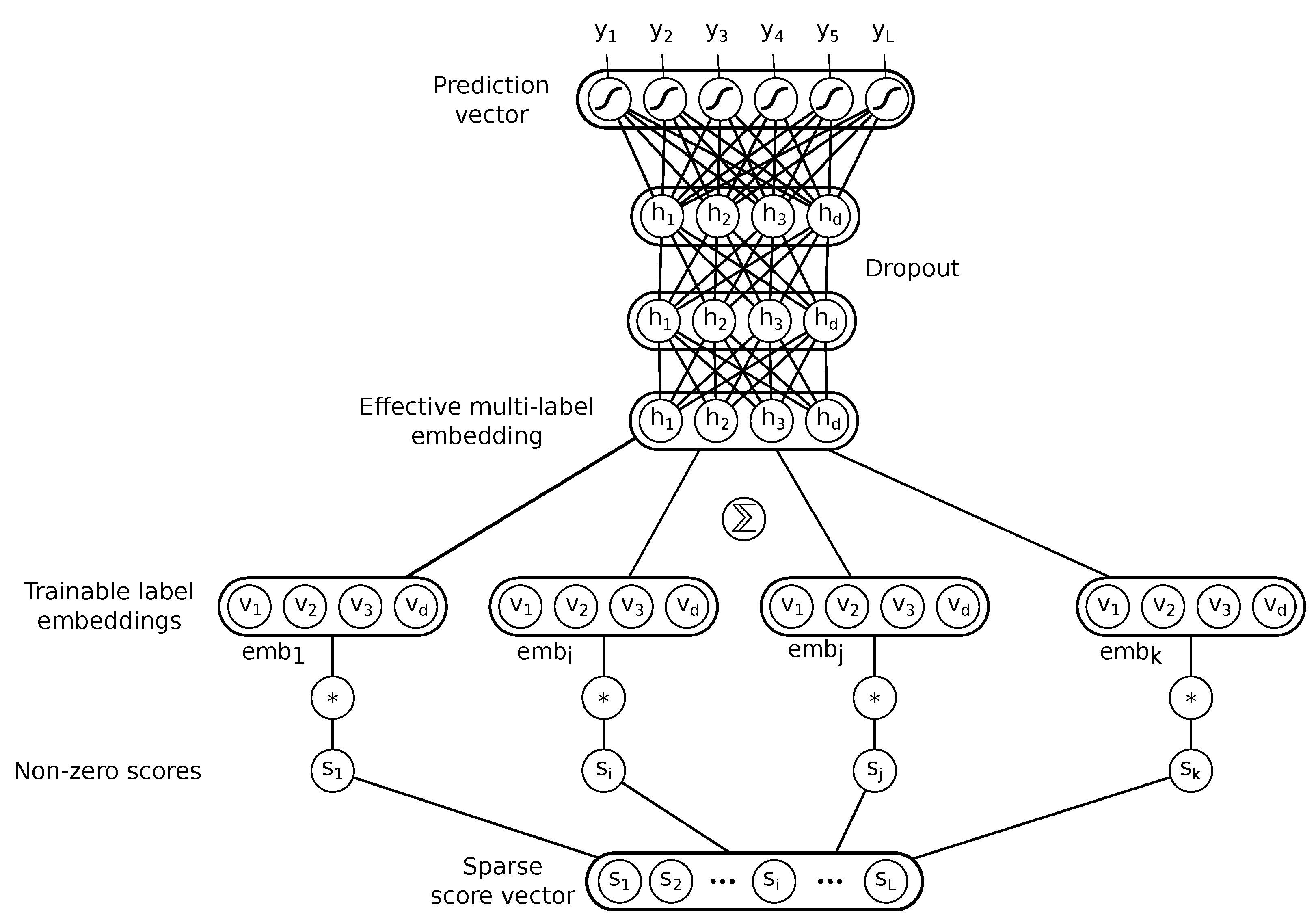
To overcome the space complexity problem of the above naive model, we propose a different architecture, presented in Figure 2, inspired by a FastText model [43]. In this model, each label is associated with a trainable label embedding (such as word embeddings in FastText), which is a vector of d floating point values. For a given input, which is a scaled score vector ss, the model calculates the effective multi-label embedding  h , which can be described as a result of sparse vector–dense matrix multiplication: h = s s · Emb , where Emb is an L × d matrix with the i-th label embedding in its i-th row. In other words, the effective multi-label embedding is a weighted sum of the label embeddings (not a simple average of the embeddings, as in the original FastText), with label scores as the weights of the components. This way, it includes information about which labels are involved in a given input as well as the intensity of these labels in the mix, as judged by a source scorer.
This multi-label embedding could be directly used to produce prediction vectors via a dense layer with L output units. After initial experiments, we found that slightly better results are possible with a deeper model. The final model has two additional hidden layers, both having d units (the same sizes as embeddings), and using the popular ReLU [44] activation function ( f ReLU ( z ) = max 0 , z ). The final model realizes the following function:
ThresNet ( ss ) = σ dense dense ReLU dense ReLU ss · Emb
For training purposes, the Heaviside is replaced by sigmoid  σ ( · ) ( σ ( z ) = 1 / 1 + exp ( z ) ), which enables a standard gradient-based training. During inference, the Heaviside function is used again to achieve binary predictions.
The presented architecture enables complex, nonlinear, and non-obvious thresholding, while having O ( d L ) complexity, where d < < L . Dimensionality of label embeddings d (which is also the hidden layer size), is the main hyperparameter for controlling the complexity of the model.
ThresNet, while inspired by FastText, is considerably different. First, the purposes of these models are different: thresholding for ThresNet versus representation learning or end-to-end classification for FastText. The main consequence of that is the nature of the model inputs: ThresNet obtains label scores and not raw feature vectors (especially not features from a fixed-sized moving context window). Second, ThresNet calculates a weighted average of label embeddings, while FastText calculates a simple average of feature embeddings. Third, ThresNet includes a couple of bottleneck hidden layers to mitigate the O ( L 2 ) complexity and improve performance, while FastText maps averaged embeddings directly into the output space. Finally, the ThresNetCSS variant, described below, is the enhancement that does not have any equivalent counterpart in FastText (and which is rather impossible, because input and output spaces are different in sizes there).

4.3. ThresNetCSS—A Residual Variant

ThresNet can learn complex patterns for seemingly easy tasks of thresholding score vectors. Although this ability is crucial to be able to correctly predict mis-scored labels, making a prediction about a label should fundamentally be based on its label score. However, ThresNet architecture does not allow for this easily, because there is no direct connection between the i-th input ss [ i ] and the i-th output y ^ [ i ] . The signal between these units has to go through three bottleneck layers and nonlinearities of activation functions.
ThresNetCSS, depicted in Figure 3, is a variant designed specifically to remedy the aforementioned problem. The idea here is to combine the powerfulness of ThresNet with traditional CS-cut thresholding, implemented as CS-net (shown in Figure 1a and Equation (12)). The model adds the input score vector just before the final activation function of ThresNet, transforming the architecture into a form of a residual network [45]. The residual connection joins the corresponding elements of large sparse input and output vectors, which are otherwise connected through bottleneck layers, similar to what is done to images in UNet-like image segmentation models [46].
Additionally, it is possible to transfer knowledge from a CS(S)-cut traditional strategy into the model via a non-trainable bias vector t C S S . The overall function of the model is as follows:
ThresNet CSS ( ss ) = σ dense dense ReLU dense ReLU Emb · ss ThresNet   part + ss t C S S CS - Net   part
During training, this residual model learns to exhibit behaviors that differ from simply applying a priori-given CSS-cut thresholds. The intuition is that complex pattern-based thresholding should be applied only when it outweighs the default CSS-cut strategy. The space complexity of ThresNetCSS is the same as the primary ThresNet.

4.4. Network Training

The presented models are trained in a standard way using stochastic gradient descent with mini-batches to minimize binary cross-entropy loss for each label:
J = 1 N i = 1 N y ( i ) log y ^ ( i ) + 1 y ( i ) log 1 y ^ ( i ) ,
where y ^ ( i ) is the model response given the i-th train-scaled score vector ss ( i ) . To minimize this loss, we used the NAdam optimizer [47] with the default settings.
In experiments on real datasets (Section 5.2), 10-fold cross-validation was employed. Partitioning data into stratified folds, which is challenging in multi-label problems, was conducted using iterative stratification described in [48]; this stratification is publicly available alongside the data [49]. To prevent overfitting, the dropout [50] layer was added to the models before the final prediction layer and early stopping was used by monitoring the loss on the validation data. In each data fold, we ran 10 trials of random searches for the best hyperparameters; thus, we trained 100 models for each dataset to select the best ones based on validation results. The whole code was implemented in Python using a TensorFlow 2.0 framework and is available at github.com/szarakawka/nn-thresholding, (accessed on 26 May 2023).

5. Experiments and Results

To have a better understanding of various thresholding strategies, i.e., the strong and weak sides, before experimenting on real datasets, we first created artificial score datasets 𝒟s and tested thresholding methods on these.
Using artificial datasets, it is possible to check the behaviors of thresholding strategies under controlled conditions. In particular, we can see and measure when and to what degree thresholding methods are able to recover correct label predictions from scoring errors.

5.1. Synthetic Scores

5.1.1. Score Generator

Synthetic data are generated using the pseudo-restricted Boltzmann machine (RBM) model, where a visible vector y i (the ground truth label vector) depends on a random one-hot hidden vector h i according to:
y i = t S-cut σ h i W ,
where σ is a sigmoid function, W is a weight matrix with real random values set once at the beginning of the generation process, sampled uniformly from range [ 1 , 1 ] , and t S-cut is the S-cut threshold function. Its single global threshold value is set to obtain the desired sparsity of label vectors (95% in our experiments). The idea behind such a pseudo-multi-label generator is that it models various correlation patterns between labels, which are encoded in the rows of W , which show off one per example in the actual data, depending on the position of 1 in a particular h i .
Importantly, ground truth label vectors are then corrupted by randomly substituting 0 s with 1 s (with a chosen False Positive Ratio (FPR)) and 1 s with 0 s (according to the specified False Negative Ratio (FNR)). score vectors are then created from the corrupted label vectors by adding Gaussian noise and pruning negative scores to 0:
s i = max corrupt ( y i ) + N ( 0 , ζ ) , 0 ,
where the standard deviation of the Gaussian ζ is a noise level and the corrupt ( · ) function is the label corruption process described above.

5.1.2. Results

Figure 4 shows the performances of traditional thresholding methods as well as ThresNets on synthetic data. The generated datasets are not imbalanced so the macro- and micro-averaged F1 scores are very similar and only macro-F1 scores are presented. For each FPR-FNR combination, a new data generator instance was created. The methods were then trained on 10,000 samples, and tested on 1000 new samples generated from the same instance. The same train and test samples are used across all the methods. The test metrics are shown.
As can be seen, for all combinations of FPR and FNR, neural thresholding performs comparable to—or much better than—the competition. Traditional methods work reasonably well when scores have high quality, i.e., the Gaussian noise added to scores is low; FPR and FNR are also very low. The performances of the baseline methods quickly drop when the score variances increase or the scores are corrupted.
The important thing to notice here is the asymmetry of the impact of FPR versus FNR on the results of the traditional methods. If FPR is small (≤0.1) and the score noise is low, they work reasonably well, even for FNR, up to 0.3. However, when FNR is low and FPR is high, this is not the case. Even for FPR = 0.1, the results are poor. Fortunately, in manually labeled real large/extreme datasets, the first scenario is much more prevalent: failing to assign all relevant labels to a given sample out of the plethora of possibilities is much more frequent than assigning an incorrect label. Still, for all FNR > 0 , the traditional methods are worse than ThresNet in this experiment.
The explanation is that due to the simplicity of traditional methods, they do not have any reconstruction abilities and they rely solely on the quality of per-label scores in isolation from the global view of label scores. In the case where a reconstruction from bad scoring is possible, normal thresholding methods are at a clear disadvantage compared to more powerful neural networks. ThresNets exhibit rethinking abilities (to use phrasing from [38]), but they do it effectively, without directly modeling all L 2 relations. The question pertains to the extent of inter-score relationships observed in real datasets obtained using authentic scorers.

5.2. Real Datasets

5.2.1. Datasets

To answer the above question, we performed experiments on two medium-sized multi-label real datasets: Eurlex dataset (EURLex4K) [51] and Simple English Wikipedia Dataset (SimpleWiki2K) [49]. The statistics of these datasets are given in Table 1.
We used two classic classifiers (scorers) to obtain score datasets: a simple k-Nearest Neighbors (k-NN) with the multi-label scoring system described in [52] and LEML [53], as a classic representative of a modern, embedding-based, extreme, multi-label classifier. After training both scorers on both train datasets, we obtained four distinct thresholding training datasets (see Section 2.3): SimpleWiki 2 K KNN , SimpleWiki 2 K LEML , EURLex 4 K KNN , and EURLex 4 K LEML .

5.2.2. Methods

We compare ThresNet and ThresNetCSS with the CSS-cut strategy, as the most powerful baseline thresholding method. We present the results of the best models selected according to the validation metrics (models denoted as single) as well as the results of the hard-voting ensemble of all 10 models, one from each fold. We also use neural-traditional hybrid models, constructed as follows: for each class separately, a thresholding method is chosen between CSS and ThresNet based on the validation performance for this class averaged over validation folds.

5.2.3. Quantitative Results

In Table 2 and Table 3, we present the results of the four described score datasets on held-out test splits. In almost all cases, ThresNetCSS performed best between single models and ensembles. According to Favg, the method turned out to be better than the best traditional method in all cases, with improvements ranging from 0.01 ( EURLex 4 K LEML ) to 0.09 ( SimpleWiki 2 K LEML ). Interestingly, sometimes the hybrid ThresNetCSS with CSS was profitable, although ThresNetCSS used CSS thresholds internally.
Higher Favg achieved by neural thresholding can be attributed to much better Fmi. Neural nets naturally optimize for Fmi because training is performed example by example, and the optimization is conducted for all labels simultaneously; each output unit participates in the binary cross entropy. On the other hand, the CSS-cut strategy fits each threshold per label separately, so it optimizes a Fma metric. In fact, with the exception of SimpleWiki 2 K LEML , CSS is much better than our neural methods (excluding hybrids) in terms of this metric. The addition of CSS priors in ThresNetCSS improves Fma considerably, but it still was not enough to reach CSS in this metric. We speculate that the main reason for the fact that a better Fmi does not entail a better Fma is that output neurons responsible for predictions for the smallest classes received few positive examples to correctly set their weights. This does not affect micro-averaged metrics much, but it does affect macro-F1 a lot, because there are many underrepresented classes, especially in the EURLex4K dataset.
The results of the held-out test sets are similar to values obtained on validation folds during cross-validation. Box plots in Figure 5 indicate that the results and characteristics of ThresNet and CSS-cut strategies are consistent over data folds. However, it can be seen that neural models, being much more complex models, exhibit slightly larger performance variations than CSS. This is why the hybrid models, for each label, decide whether it is beneficial to use a ThresNet or just CSS, based on the average of the validation folds.

5.2.4. Qualitative Results

To show the capability of ThresNet to recover from label-level scoring mistakes, we present some successful recoveries from extreme mis-scorings found in the test samples.
Table 4 presents a case of an article with a 0 score for its correct label, which means that whatever classical thresholding strategy is used, it will certainly fail to provide the correct prediction. Nevertheless, ThresNetCSS predicted the label based on scores associated with other labels. Similarly, Table 5 shows a case where incorrect labels have, by far, the largest scores, where classical thresholding strategies would again fail by returning a couple of false positives, but ThresNetCSS was able to make a correct prediction.
These are just two cases of extreme recovery, which are not very frequent. However, there are many less spectacular (but important) corrections; for example, when a correct class had a relatively low score compared to the scores of incorrect labels. Such recoveries were not possible for other thresholding techniques. Once again, only the rethinking structure [38] would be able to achieve a similar effect if it is successfully scaled to thousands of labels.

6. Conclusions

In this paper, we proposed two variants of a novel neural network-based thresholding method for obtaining high-quality multi-label predictions from class scores already available from external scorers. Our models, called ThresNets, are designed to scale linearly with the number of labels and can be trained offline entirely, e.g., after the training of a scorer is finished. The second variant of our proposal shows a way to incorporate classic CS/CSS thresholds into the neural model, which can be viewed as a kind of transfer learning between heterogeneous models. The presented thresholding methods exhibit interesting recovering possibilities from scoring errors that are unavailable in classic approaches.
Our method is well suited for middle-sized MLC tasks, where the label space is large enough, such that informative dependencies between label scores can be found, and the ground truth of label assignments is still reliable (which is problematic in XMLC problems). Our experiments on artificially created scores show that the complex thresholding phase can be especially beneficial when the scoring phase leaves enough room for improvements. For example, popular nearest neighbor-based classifiers (such as k-NN and LEML, among others) may produce underscored or overscored labels due to their use of local information about the instance. In such cases, ThresNets proved to be useful.
In our empirical evaluation on real datasets, ThresNets clearly show better performances according to Favg, Fmi, as part of a hybrid with classical methods, Fma metrics, tested on four dataset–scorer combinations, as well as on synthetic datasets. Among single thresholding methods, we had up to 40.6% relative improvement over the CSS-cut baseline in Fmi (0.6 over 0.43), 3.6% relative improvement in Fma (0.174 over 0.168), and 30.1% relative improvement (0.389 over 0.299) in Favg (the results for SimpleWiki 2 K LEML scores).
Among the downsides of the proposed methods, one of the hardest to overcome is the risk of overfitting to training data. We attempted to minimize this risk by using regularization methods while training neural models (dropout layer, early stopping, cross-validation) as well as designing ThresNetCSS architecture that learns only the residuals over the CSS-cut baseline. Still, the abundance of long-tail labels, for which only a few positive samples are available, makes the training hard, and we found that a hybrid of ThresNetCSS and the CSS-cut strategy often works better than ThresNetCSS only.
In the future, we will utilize the external knowledge of class structure by encoding it in label embeddings. We can then start ThresNet training with such prepared embeddings instead of random ones, as is currently done. Intuitively, when such a structure exists (e.g., Wikipedia (pseudo)-hierarchy of categories), encoding it in pretrained label embeddings should be beneficial, and our models can make use of them without any changes in architecture. This external knowledge could also be used in a more complicated way, for example, to initialize an additional sparsely connected first layer, where instead of a dense matrix W , there would be, e.g., a sparse category graph adjacency matrix of a fixed structure, with trainable weights. Another potential extension of the presented neural models is to make them work on scores obtained not only from one scorer but from two or more scorers at the same time; in this way, they can work as merging units trained to produce optimal predictions based on available scorers. Yet another interesting direction of the development of ThresNets is to include hierarchy-related cost-sensitivity (see e.g., [19,54,55]) while training them, enabling better performance in terms of hierarchical classification metrics. Sometimes hierarchical organization of categories may change; if so, it would be faster to fine-tune a thresholding phase than retrain the whole classification system.

Author Contributions

Conceptualization, K.D. and J.S.; methodology, K.D. and J.S.; software, K.D.; validation, K.D.; data curation, K.D.; writing—original draft preparation, K.D.; writing—review and editing, K.D. and J.S.; supervision, J.S. All authors have read and agreed to the published version of the manuscript.

Funding

This research was funded by Faculty of Electronics, Telecommunications and Informatics, Gdansk University of Technology.

Informed Consent Statement

Not applicable.

Data Availability Statement

The SimpleWiki2K dataset was created during the development of the project and is publicly available at https://doi.org/10.34808/fmnf-4767, (accessed on 26 May 2023) [49]. The EURLex4K dataset is available from the extreme classification repository [22].

Conflicts of Interest

The authors declare no conflict of interest.

Abbreviations

The following abbreviations are used in this manuscript:
k-NNk-Nearest Neighbors
EURLex4KEurlex dataset
FNRFalse Negative Ratio
FPRFalse Positive Ratio
LEMLLow-rank Empirical risk minimization for Multi-Label Learning
MLCMulti-Label Classification
SimpleWiki2KSimple English Wikipedia Dataset
XMLCeXtreme Multi-Label Classification

References

  1. Partalas, I.; Kosmopoulos, A.; Baskiotis, N.; Artières, T.; Paliouras, G.; Gaussier, E.; Androutsopoulos, I.; Amini, M.R.; Gallinari, P. LSHTC: A Benchmark for Large-Scale Text Classification. Available online: https://hal.science/hal-01691460 (accessed on 26 May 2023).
  2. Jiang, T.; Wang, D.; Sun, L.; Yang, H.; Zhao, Z.; Zhuang, F. LightXML: Transformer with Dynamic Negative Sampling for High-Performance Extreme Multi-label Text Classification. Proc. Aaai Conf. Artif. Intell. 2021, 35, 7987–7994. [Google Scholar] [CrossRef]
  3. Vu, H.T.; Nguyen, M.T.; Nguyen, V.C.; Pham, M.H.; Nguyen, V.Q.; Nguyen, V.H. Label-representative graph convolutional network for multi-label text classification. Appl. Intell. 2022, 53, 14759–14774. [Google Scholar] [CrossRef]
  4. Ma, Y.; Liu, X.; Zhao, L.; Liang, Y.; Zhang, P.; Jin, B. Hybrid embedding-based text representation for hierarchical multi-label text classification. Expert Syst. Appl. 2022, 187, 115905. [Google Scholar] [CrossRef]
  5. Khataei Maragheh, H.; Gharehchopogh, F.S.; Majidzadeh, K.; Sangar, A.B. A New Hybrid Based on Long Short-Term Memory Network with Spotted Hyena Optimization Algorithm for Multi-Label Text Classification. Mathematics 2022, 10, 488. [Google Scholar] [CrossRef]
  6. Maltoudoglou, L.; Paisios, A.; Lenc, L.; Martínek, J.; Král, P.; Papadopoulos, H. Well-calibrated confidence measures for multi-label text classification with a large number of labels. Pattern Recognit. 2022, 122, 108271. [Google Scholar] [CrossRef]
  7. Lin, T.Y.; Maire, M.; Belongie, S.; Hays, J.; Perona, P.; Ramanan, D.; Dollár, P.; Zitnick, C.L. Microsoft coco: Common objects in context. In Proceedings of the Computer Vision—ECCV 2014: 13th European Conference, Zurich, Switzerland, 6–12 September 2014; pp. 740–755. [Google Scholar]
  8. Kundalia, K.; Patel, Y.; Shah, M. Multi-label Movie Genre Detection from a Movie Poster Using Knowledge Transfer Learning. Augment. Hum. Res. 2020, 5, 11. [Google Scholar] [CrossRef]
  9. Kuznetsova, A.; Rom, H.; Alldrin, N.; Uijlings, J.; Krasin, I.; Pont-Tuset, J.; Kamali, S.; Popov, S.; Malloci, M.; Kolesnikov, A.; et al. The open images dataset v4: Unified image classification, object detection, and visual relationship detection at scale. Int. J. Comput. Vis. 2020, 128, 1956–1981. [Google Scholar] [CrossRef] [Green Version]
  10. Cheng, X.; Lin, H.; Wu, X.; Shen, D.; Yang, F.; Liu, H.; Shi, N. Mltr: Multi-label classification with transformer. In Proceedings of the 2022 IEEE International Conference on Multimedia and Expo (ICME), Taipei, Taiwan, 18–22 July 2022; pp. 1–6. [Google Scholar]
  11. Liang, J.; Xu, F.; Yu, S. A multi-scale semantic attention representation for multi-label image recognition with graph networks. Neurocomputing 2022, 491, 14–23. [Google Scholar] [CrossRef]
  12. Fonseca, E.; Plakal, M.; Font, F.; Ellis, D.P.W.; Serra, X. Audio tagging with noisy labels and minimal supervision. In Proceedings of the Submitted to DCASE2019 Workshop, New York, NY, USA, 25–26 October 2019. [Google Scholar]
  13. Ykhlef, H.; Diffallah, Z.; Allali, A. Ensembling Residual Networks for Multi-Label Sound Event Recognition with Weak Labeling. In Proceedings of the 2022 7th International Conference on Image and Signal Processing and their Applications (ISPA), Mostaganem, Algeria, 8–9 May 2022; pp. 1–6. [Google Scholar]
  14. Aironi, C.; Cornell, S.; Principi, E.; Squartini, S. Graph Node Embeddings for ontology-aware Sound Event Classification: An evaluation study. In Proceedings of the 2022 30th European Signal Processing Conference (EUSIPCO), Belgrade, Serbia, 29 August–2 September 2022; pp. 414–418. [Google Scholar]
  15. Liu, W.; Ren, Y.; Wang, J. Attention Mixup: An Accurate Mixup Scheme Based On Interpretable Attention Mechanism for Multi-Label Audio Classification. In Proceedings of the ICASSP 2023—2023 IEEE International Conference on Acoustics, Speech and Signal Processing (ICASSP), Rhodes Island, Greece, 4–10 June 2023. [Google Scholar]
  16. Zhong, Z.; Hirano, M.; Shimada, K.; Tateishi, K.; Takahashi, S.; Mitsufuji, Y. An Attention-Based Approach to Hierarchical Multi-Label Music Instrument Classification. In Proceedings of the ICASSP 2023—2023 IEEE International Conference on Acoustics, Speech and Signal Processing (ICASSP), Rhodes Island, Greece, 4–10 June 2023. [Google Scholar]
  17. Wang, X.; Zhao, H.; Lu, B.L. Enhanced K-Nearest Neighbour Algorithm for Large-scale Hierarchical Multi-label Classification. In Proceedings of the Joint ECML/PKDD PASCAL Workshop on Large-Scale Hierarchical Classification, Athens, Greece, 5 September 2011; p. 58. [Google Scholar]
  18. Draszawka, K.; Szymański, J. Thresholding strategies for large scale multi-label text classifier. In Proceedings of the 6th International Conference on Human System Interaction (HSI), Sopot, Poland, 6–8 June 2013; pp. 350–355. [Google Scholar]
  19. Liu, Y.; Li, Q.; Wang, K.; Liu, J.; He, R.; Yuan, Y.; Zhang, H. Automatic multi-label ECG classification with category imbalance and cost-sensitive thresholding. Biosensors 2021, 11, 453. [Google Scholar] [CrossRef] [PubMed]
  20. Li, J.; Li, P.; Hu, X.; Yu, K. Learning common and label-specific features for multi-Label classification with correlation information. Pattern Recognit. 2022, 121, 108259. [Google Scholar] [CrossRef]
  21. Haghighian Roudsari, A.; Afshar, J.; Lee, W.; Lee, S. PatentNet: Multi-label classification of patent documents using deep learning based language understanding. Scientometrics 2022, 127, 207–231. [Google Scholar] [CrossRef]
  22. Bhatia, K.; Dahiya, K.; Jain, H.; Mittal, A.; Prabhu, Y.; Varma, M. The Extreme Classification Repository: Multi-Label Datasets and Code. Available online: http://manikvarma.org/downloads/XC/XMLRepository.html (accessed on 26 May 2023).
  23. Agrawal, R.; Gupta, A.; Prabhu, Y.; Varma, M. Multi-label learning with millions of labels: Recommending advertiser bid phrases for web pages. In Proceedings of the 22nd international conference on World Wide Web, Rio de Janeiro, Brazil, 13–17 May 2013; pp. 13–24. [Google Scholar]
  24. Jain, H.; Prabhu, Y.; Varma, M. Extreme multi-label loss functions for recommendation, tagging, ranking & other missing label applications. In Proceedings of the 22nd ACM SIGKDD International Conference on Knowledge Discovery and Data Mining, San Francisco, CA, USA, 13–17 August 2016; pp. 935–944. [Google Scholar]
  25. Prabhu, Y.; Kag, A.; Harsola, S.; Agrawal, R.; Varma, M. Parabel: Partitioned label trees for extreme classification with application to dynamic search advertising. In Proceedings of the 2018 World Wide Web Conference, Lyon, France, 23–27 April 2018; pp. 993–1002. [Google Scholar]
  26. Jain, H.; Balasubramanian, V.; Chunduri, B.; Varma, M. Slice: Scalable linear extreme classifiers trained on 100 million labels for related searches. In Proceedings of the Twelfth ACM International Conference on Web Search and Data Mining, Melbourne, Australia, 11–15 February 2019; pp. 528–536. [Google Scholar]
  27. Medini, T.K.R.; Huang, Q.; Wang, Y.; Mohan, V.; Shrivastava, A. Extreme classification in log memory using count-min sketch: A case study of amazon search with 50m products. In Proceedings of the 32nd Annual Conference on Neural Information Processing Systems 2019, NeurIPS 2019, Vancouver, BC, Canada, 8–14 December 2019; pp. 13244–13254. [Google Scholar]
  28. Ye, H.; Chen, Z.; Wang, D.H.; Davison, B. Pretrained generalized autoregressive model with adaptive probabilistic label clusters for extreme multi-label text classification. In Proceedings of the International Conference on Machine Learning, Virtual Event, 13–18 July 2020; pp. 10809–10819. [Google Scholar]
  29. Saini, D.; Jain, A.K.; Dave, K.; Jiao, J.; Singh, A.; Zhang, R.; Varma, M. GalaXC: Graph neural networks with labelwise attention for extreme classification. In Proceedings of the Web Conference 2021, Ljubljana, Slovenia, 12–13 April 2021; pp. 3733–3744. [Google Scholar]
  30. Mittal, A.; Dahiya, K.; Malani, S.; Ramaswamy, J.; Kuruvilla, S.; Ajmera, J.; Chang, K.H.; Agarwal, S.; Kar, P.; Varma, M. Multi-modal extreme classification. In Proceedings of the IEEE/CVF Conference on Computer Vision and Pattern Recognition, New Orleans, LA, USA, 21–14 June 2022; pp. 12393–12402. [Google Scholar]
  31. Dahiya, K.; Gupta, N.; Saini, D.; Soni, A.; Wang, Y.; Dave, K.; Jiao, J.; Dey, P.; Singh, A.; Hada, D.; et al. NGAME: Negative Mining-aware Mini-batching for Extreme Classification. In Proceedings of the 16th ACM International Conference on Web Search and Data Mining, Singapore, 27 February–3 March 2023; pp. 258–266. [Google Scholar]
  32. Yang, Y. A study of thresholding strategies for text categorization. In Proceedings of the 24th Annual International ACM SIGIR Conference on Research and Development in Information Retrieval, New Orleans, LA, USA, 9–13 September 2001; pp. 137–145. [Google Scholar]
  33. Triguero, I.; Vens, C. Labelling strategies for hierarchical multi-label classification techniques. Pattern Recognit. 2016, 56, 170–183. [Google Scholar] [CrossRef] [Green Version]
  34. Quevedo, J.R.; Luaces, O.; Bahamonde, A. Multilabel classifiers with a probabilistic thresholding strategy. Pattern Recognit. 2012, 45, 876–883. [Google Scholar] [CrossRef] [Green Version]
  35. Lewis, D.D. An evaluation of phrasal and clustered representations on a text categorization task. In Proceedings of the 15th Annual International ACM SIGIR Conference on Research and Development in Information Retrieval, Copenhagen, Denmark, 21–24 June 1992; pp. 37–50. [Google Scholar]
  36. Li, L.; Wang, H.; Sun, X.; Chang, B.; Zhao, S.; Sha, L. Multi-label text categorization with joint learning predictions-as-features method. In Proceedings of the 2015 Conference on Empirical Methods in Natural Language Processing, Lisbon, Portugal, 17–21 September 2015; pp. 835–839. [Google Scholar]
  37. Wu, J.; Xiong, W.; Wang, W.Y. Learning to Learn and Predict: A Meta-Learning Approach for Multi-Label Classification. In Proceedings of the 2019 Conference on Empirical Methods in Natural Language Processing and the 9th International Joint Conference on Natural Language Processing (EMNLP-IJCNLP), Hong Kong, China, 3–7 November 2019; pp. 4354–4364. [Google Scholar] [CrossRef]
  38. Yang, Y.Y.; Lin, Y.A.; Chu, H.M.; Lin, H.T. Deep learning with a rethinking structure for multi-label classification. In Proceedings of the Asian Conference on Machine Learning, PMLR, Nagoya, Japan, 17–19 November 2019; pp. 125–140. [Google Scholar]
  39. Huang, J.; Huang, A.; Guerra, B.C.; Yu, Y. PercentMatch: Percentile-based Dynamic Thresholding for Multi-Label Semi-Supervised Classification. arXiv 2022, arXiv:2208.13946. [Google Scholar] [CrossRef]
  40. Liu, S.; Zhang, L.; Yang, X.; Su, H.; Zhu, J. Query2Label: A Simple Transformer Way to Multi-Label Classification. arXiv 2021, arXiv:2107.10834. [Google Scholar] [CrossRef]
  41. Ridnik, T.; Sharir, G.; Ben-Cohen, A.; Ben-Baruch, E.; Noy, A. Ml-decoder: Scalable and versatile classification head. In Proceedings of the IEEE/CVF Winter Conference on Applications of Computer Vision, Waikoloa, HI, USA, 2–7 January 2023; pp. 32–41. [Google Scholar]
  42. Gray, S.; Radford, A.; Kingma, D.P. Gpu Kernels for Block-Sparse Weights. 2017. Available online: https://openai.com/research/block-sparse-gpu-kernels (accessed on 26 May 2023).
  43. Joulin, A.; Grave, E.; Bojanowski, P.; Mikolov, T. Bag of Tricks for Efficient Text Classification. In Proceedings of the 15th Conference of the European Chapter of the Association for Computational Linguistics: Volume 2, Short Papers, Valencia, Spain, 3–7 April 2017; pp. 427–431. [Google Scholar]
  44. Nair, V.; Hinton, G.E. Rectified linear units improve restricted boltzmann machines. In Proceedings of the International Conference on Machine Learning, Haifa, Israel, 21–24 June 2010; pp. 807–814. [Google Scholar]
  45. He, K.; Zhang, X.; Ren, S.; Sun, J. Deep residual learning for image recognition. In Proceedings of the IEEE Conference on Computer Vision and Pattern Recognition, Las Vegas, NV, USA, 27–30 June 2016; pp. 770–778. [Google Scholar]
  46. Ronneberger, O.; Fischer, P.; Brox, T. U-net: Convolutional networks for biomedical image segmentation. In Proceedings of the International Conference on Medical Image Computing and Computer-Assisted Intervention, Munich, Germany, 5–9 October 2015; pp. 234–241. [Google Scholar]
  47. Dozat, T. Incorporating nesterov momentum into adam. In Proceedings of the 4th International Conference on Learning Representations: Workshop Track, San Juan, Puerto Rico, 2–4 May 2016; pp. 1–4. [Google Scholar]
  48. Sechidis, K.; Tsoumakas, G.; Vlahavas, I. On the stratification of multi-label data. In Proceedings of the Joint European Conference on Machine Learning and Knowledge Discovery in Databases, Athens, Greece, 5–9 September 2011; pp. 145–158. [Google Scholar]
  49. Draszawka, K.; Boiński, T.; Szymański, J. TF-IDF Weighted Bag-of-Words Preprocessed Text Documents from Simple English Wikipedia. 2023. Available online: https://mostwiedzy.pl/en/open-research-data/tf-idf-weighted-bag-of-words-preprocessed-text-documents-from-simple-english-wikipedia,42511260848405-0 (accessed on 26 May 2023).
  50. Srivastava, N.; Hinton, G.; Krizhevsky, A.; Sutskever, I.; Salakhutdinov, R. Dropout: A simple way to prevent neural networks from overfitting. J. Mach. Learn. Res. 2014, 15, 1929–1958. [Google Scholar]
  51. Mencia, E.L.; Fürnkranz, J. Efficient pairwise multilabel classification for large-scale problems in the legal domain. In Proceedings of the Joint European Conference on Machine Learning and Knowledge Discovery in Databases, Antwerp, Belgium, 15–19 September 2008; pp. 50–65. [Google Scholar]
  52. Han, X.; Li, S.; Shen, Z. A k-NN method for large scale hierarchical text classification at LSHTC3. In Proceedings of the 2012 ECML/PKDD Discovery Challenge Workshop on Large-Scale Hierarchical Text Classification, Bristol, UK, 28 September 2012. [Google Scholar]
  53. Yu, H.F.; Jain, P.; Kar, P.; Dhillon, I. Large-scale multi-label learning with missing labels. In Proceedings of the International Conference on Machine Learning, Beijing, China, 21–26 June 2014; pp. 593–601. [Google Scholar]
  54. Alotaibi, R.; Flach, P. Multi-label thresholding for cost-sensitive classification. Neurocomputing 2021, 436, 232–247. [Google Scholar] [CrossRef]
  55. Ghaderi Zefrehi, H.; Sheikhi, G.; Altınçay, H. Threshold prediction for detecting rare positive samples using a meta-learner. Pattern Anal. Appl. 2023, 26, 289–306. [Google Scholar] [CrossRef]
Figure 1. Basic neural network thresholding models. (a) Neural network realizing the CS-cut thresholding: CS-Net; (b) naive generalization of the CS-cut thresholding.
Applsci 13 07591 g001
Figure 2. ThresNet—a thresholding model with label embeddings.
Applsci 13 07591 g002
Figure 3. ThresNetCSS—a residual variant that enables easy and simple strategic calculations and CSS-threshold priors.
Applsci 13 07591 g003
Figure 4. Test macro F1 score performance of traditional thresholding methods and ThresNets for synthetic data for various FPR and FNR: (a) low score noise level ζ = 0.02 and (b) high score noise level ζ = 0.4 . Number of labels L = 1000 , size of h = 50 .
Applsci 13 07591 g004
Figure 5. Box plots for classification metrics on validation sets for the 10-fold cross-validation of the ThresNet and CSS-cut strategies on SimpleWiki2KKNN (red boxes) and SimpleWiki2KLEML (blue boxes) datasets: (a) Fmi, (b) Fma, and (c) Favg.
Applsci 13 07591 g005
Table 1. EURLex4K and SimpleWiki2K—statistics of datasets used in the experiments.
DatasetFeature DimsLabel DimsTraining ExamplesTesting ExamplesAvg. Examples per LabelAvg. Labels per Example
SimpleWiki2K97,179184960,744676152.601.60
EURLex4K5000395615,539380920.865.31
Table 2. Thresholding results on the SimpleWiki2K test set and scores given by k-NN and LEML scorers.
Thresholding Methodk-NN ScoresLEML Scores
FmiFmaFavgFmiFmaFavg
CSS (single)0.4340.2990.3670.4290.1680.299
ThresNet (single)0.5560.2220.3890.6020.1690.386
ThresNetCSS (single)0.5920.2350.4130.6030.1740.389
CSS+ThresNet (single)0.4440.2970.3710.4700.1890.329
CSS+ThresNetCSS (single)0.4490.3040.3770.4720.1930.332
CSS (ensemble)0.4420.3080.3750.4340.1770.306
ThresNet (ensemble)0.6020.2160.4090.6220.1650.394
ThresNetCSS (ensemble)0.6080.2360.4220.6220.1690.396
CSS+ThresNet (ensemble)0.4590.3140.3870.5000.2100.355
CSS+ThresNetCSS (ensemble)0.4670.3200.3930.5020.2130.358
Table 3. Thresholding results on the EURLex4K test set and scores given by k-NN and LEML scorers.
Thresholding Methodk-NN ScoresLEML Scores
FmiFmaFavgFmiFmaFavg
CSS (single)0.3440.2110.2780.4250.1660.295
ThresNet (single)0.4330.1370.2850.4690.1410.305
ThresNetCSS (single)0.4410.1820.3110.4670.1420.305
CSS+ThresNet (single)0.3310.2060.2680.4460.1670.307
CSS+ThresNetCSS (single)0.3390.2100.2740.4470.1690.308
CSS (ensemble)0.3560.2190.2870.4280.1660.297
ThresNet (ensemble)0.4640.1440.3040.4670.1300.299
ThresNetCSS (ensemble)0.4800.1520.3160.4790.1390.309
CSS+ThresNet (ensemble)0.3540.2170.2850.4450.1710.308
CSS+ThresNetCSS (ensemble)0.3530.2150.2840.4500.1730.311
Table 4. An example of a successful classification of an extremely under-scored case: a Simple Wiki article titled List of Consadole Sapporo players.
Label Namek-NNScaledCSSThresNetCSS
ScoreScorePredictionPrediction
Living people3.7781.0FPTN
Sportspeople stubs3.7781.0FPTN
Footballers from Tokyo0.1530.041TNTN
Japan stubs0.1240.033TNTN
North Korean footballers0.0990.026TNTN
Cities in Japan0.0760.02TNTN
Lists of Japanese football players00FNTP
Table 5. An example of a successful classification of a case involving over-scored labels: an article titled Real Zaragoza.
Label Namek-NNScaledCSSThresNetCSS
ScoreScorePredictionPrediction
Living people4.791.0FPTN
Sportspeople stubs4.791.0FPTN
Sports stubs2.9610.618FNTP
Uruguayan footballers0.170.035TNTN
Croatian footballers0.1580.033TNTN
Geography stubs0.0670.014TNTN
Disclaimer/Publisher’s Note: The statements, opinions and data contained in all publications are solely those of the individual author(s) and contributor(s) and not of MDPI and/or the editor(s). MDPI and/or the editor(s) disclaim responsibility for any injury to people or property resulting from any ideas, methods, instructions or products referred to in the content.

