PEiD: Precise and Real-Time LOS/NLOS Path Identification Based on Peak Energy Index Distribution

Abstract

Wireless sensing has emerged as an innovative technology that enables many smart applications such as indoor localization, activity recognition, and user tracking. However, achieving reliable and precise results in wireless sensing requires an accurate distinction between line-of-sight and non-line-of-sight transmissions. This paper introduces PEiD, a novel method that utilizes low-cost WiFi devices for transmission path identification, offering real-time measurements with high accuracy through the application of machine-learning-based classifiers. To overcome the deficiencies of commodity WiFi in bandwidth, PEiD explores the peak energy index distribution extracted from the channel impulse responses. Our approach effectively captures the inherent randomness of channel properties and significantly reduces the number of samples required for identification, thus surpassing previous methods. Additionally, to tackle the challenge of mobility, a sliding window technique is also adopted to achieve continuous monitoring of transmission path status. According to our extensive experiments, PEiD can attain a best path identification accuracy of 97.5% for line-of-sight scenarios and 94.3% for non-line-of-sight scenarios, with an average delay of under 300 ms (92% accuracy) even in dynamic environments.

1. Introduction

Over the past decade, artificial intelligence (AI) has experienced remarkable growth across numerous research fields, including medical research [1] and the economy [2]. This technology endows machines with the ability to learn complex features from vast amounts of data and perform intricate tasks with greater intelligence. The recent emergence of the Internet of Things (IoT) has enabled the fusion of AI techniques with wireless devices, leading to the development of the AI of Things (AIoT) [3,4,5,6,7]. Wireless sensing, with its unique ability to monitor human behavior and positions using omnipresent electromagnetic waves, is gaining attention [8]. This contactless and non-intrusive sensing technique is believed to offer superior privacy protection compared to traditional camera or wearable-device-based methods. The advent of AI techniques, specifically machine learning (ML) and deep learning (DL), has enabled the exploration of intelligent applications, such as indoor positioning [9], target tracking [10], gesture recognition [11,12], and respiration monitoring [13,14].

However, a considerable number of existing studies are confined by the necessity of a line-of-sight (LOS) path. First, the existence of a LOS path is essential for device-based localization applications. This is because accurate localization is achieved by measuring the distance and angle of direct path between transceivers [15,16]. The NLOS blocking can lead to wrong parameter estimation, thus causing performance degradation. Second, a LOS path can provide a stable and noiseless channel environment so that fine-grained activity recognition can be achieved. According to previous research on WiFi sensing models [7], the received signal can be split into two parts: the static and the dynamic component. Only when the environmental reflections and LOS signals remain constant are we able to extract the features related to activity. A similar assumption exists in many works of gesture recognition based on Doppler Frequency Shift (DFS) [11,17] and Fresnel zones [12,18].

A multitude of strategies have been suggested to tackle the issue of LOS/NLOS identification. Early studies in the field focus on exploring statistical characteristics such as the mean and standard deviation of measured channel properties [19,20,21,22,23]. The rational is that the channel properties of NLOS paths exhibit more randomness than that of LOS ones, resulting in notable differences in the distribution. This type of solution is simple and effective but requires reliable measurement of range, Time of Arrival (ToA), and Angle of Arrival (AoA). Another group of works exploits the high-precision Channel Impulse Response (CIR) provided by Ultra-Wideband (UWB) technology [24,25,26,27,28,29]. It offers a feature map of superior time resolution that contains rich Multi-Path Components (MPCs) of received signals. Although UWB-based solutions can achieve excellent and stable identification performance, the high cost of UWB hardware hinders its development and application. An alternate strategy leverages the Channel State Information (CSI) provided by commodity WiFi devices [30,31,32,33,34,35,36,37]. Due to the widespread infrastructure of IoT, WiFi has attracted wide attention for its advantage in deployment. However, it still faces constraints due to bandwidth limitations and inadequate resolution. Furthermore, existing works demand a larger sample size, thereby precluding real-time LOS/NLOS identification.

In this paper, we introduce a WiFi-based LOS/NLOS identification approach called PEiD. Instead of extracting features from CSI, we investigate the CIR obtained through inverse Fast Fourier Transform (iFFT). Despite the limited bandwidth of commodity WiFi, we have found that the time index of CIR reflects the randomness of NLOS paths. To leverage this insight, we propose a novel feature called the peak energy index distribution, which has proven to be a promising indicator for identifying LOS and NLOS signals. Furthermore, we construct a machine-learning-based classifier that utilizes statistical characteristics, achieving two significant improvements over previous work. Firstly, PEiD can significantly reduce the sample size required for path identification. Even if the sample size decreases to one-fifth of the original volume, PEiD can still maintain a relatively high identification accuracy of 94% and 92.7% for LOS and NLOS cases, while the best performances are 97.5% and 94.3%. Secondly, PEiD incorporates sliding windows to handle transceiver mobility, with an identification delay of approximately 235 ms when the channel state changes. We believe this delay is adequate for home use and is acceptable for most practical applications.

The main contributions of this paper are listed below:

(1)

We adopt a novel feature called peak energy index distribution for fast and accurate LOS/NLOS identification. It exploits CIR from the time domain instead of the frequency domain. A threshold-based classifier is built to validate its effectiveness under different environments, achieving an average accuracy of 67%.

(2)

We build a machine-learning-based LOS/NLOS classifier, considering both the time and power features of CIR. Random Forest is chosen as the best-performing algorithm [38], achieving a best identification accuracy of 97.5% and 94.3% in LOS and NLOS cases, respectively.

(3)

We use a sliding window to handle transceiver mobility. Although it still requires time for data sampling, experimental results show that the delay to obtain a recognition accuracy of 95% is around 235 ms, which is acceptable for most applications.

The rest of this paper is organized as follows. Section 2 reviews related work on LOS/NLOS identification. Section 3 provides background information on CSI and CIR, as well as introduces the concept of peak energy index distribution. Section 4 details our proposed PEiD approach, which comprises both a threshold-based variant and a machine-learning-based version. An extended version of PEiD is also introduced to handle transceiver mobility using a sliding window. Section 5 presents the experimental results of the proposed method in a real-world application and compares its performance with previous work. Finally, Section 6 concludes the paper with some remarks and future research directions.

2. Related Work

Prior research in the field focuses on exploring the random nature of NLOS paths through a range of specific parameters measured from the received signal. These parameters include range [20], ToA [22,23], Received Signal Strength (RSS) [21], and AoA [19]. As unstable channel properties of NLOS can severely disturb the measurement of the parameter, researchers can determine the NLOS paths by capturing abnormal values. For instance, Momtaz et al. [20] model the NLOS error as a deterministic additive term in addition to a white zero-mean Gaussian noise. Autocorrelation and eigenvector analyses are adopted to find the error. Aghaie et al. [19] investigate AoA measurements of Wireless Sensor Networks (WSN) and adopt the theorem of Neyman–Pearson to detect the occurrence of abnormal values. To reduce the errors caused by NLOS paths, Krishna Das et al. [22] propose an NLOS identification and mitigation method based on a Kalman Filter (KF). For more accurate NLOS identification, other researchers also exploit techniques of machine learning such as Support Vector Machines (SVM) [23] and neural networks [21].

The idea of statistics-based solutions is simple and effective. However, their methods may not be applicable to WiFi sensing. First, some of the works mentioned above are based on cellular networks and WSNs. Their application scenarios can be different from that of WiFi in indoor environments. Second, due to the limitation on bandwidth, most commodity WiFi devices are not able to provide reliable measurements of ToA or AoA. That increases the difficulty of detecting NLOS errors.

Distinct from the approaches based on statistical parameters, UWB-based solutions focus on extracting features from CIR [24,25,26,27,28,29,39]. Early works tend to assess the energy decay and time delay caused by NLOS obstructions. When the LOS path is obstructed, the signal can only reach the receiver through reflection, resulting in a longer propagation distance and more power loss. They use kurtosis and K-Factor to reflect the CIR energy distribution while using Root Mean Delay Spread (RMS) and Mean Excess Delay (MED) to describe the time characteristics [24,39]. Based on commercial UWB chips, Ferreira et al. [29] further design thirteen features and select a subset to achieve the best performance. More recent works take advantage of deep neural networks, such as Multi-Layer Perceptions (MLP), Convolutional Neural Networks (CNN), and Long Short-Term Memory (LSTM) networks, to learn more complex features from CIR [25,26,28]. However, the complex model training also raises the issue of laborious data collection. Dong et al. [27] propose a low-cost NLOS identification method to mitigate the problem. By utilizing the Fresnel zones theory, their approach can work in variable environments without much data collection.

UWB devices offer remarkable accuracy due to their extensive bandwidth resources (over 1 GHz), which provide superior time resolution for CIR measurements. Thus, UWB devices are capable of detecting slight changes in the time delay of the received signal, thereby uncovering the tiny differences in propagation distance. However, the high cost of UWB hardware is a defect that cannot be ignored. Although there are already some commercial UWB chips on the market, the deployment of UWB devices is still not as convenient as WiFi.

WiFi-based solutions extract features from CSI, which carries both magnitude and phase information. For instance, LiFi [30] explores the statistic parameters of CSI and CIR magnitude. The authors use the Rician-K factor and skewness to capture characteristics of CIR envelope distribution. Their proposed method achieves an identification accuracy of 90.4% by introducing mobility to increase the channel randomness. However, LiFi requires a large sample size of 500–2000 packets for each identification, resulting in a time delay of 1–4 s when transmitting packets at a frequency of 500 Hz. PhaseU [31] explores the phase values of CSI by eliminating the random phase offset through the signal differential. The authors compute the variance of phase difference and adopt a threshold-based classifier to achieve NLOS identification, whose accuracy is 94%. Although PhaseU allows users to move during identification, it can only collect samples after the receiver remain static. An extra inertial sensor is required to detect the user’s motion status, making PhaseU unable to achieve real-time identification.

To further investigate the characteristic of CSI, other WiFi-based approaches also adopt deep learning models. Xiao et al. [32] utilizes a neural network to analyze CSI magnitude. Choi et al. [33] leverage a Recurrent Neural Network (RNN) to extract temporal features of CSI and RSS sequence. Zhu et al. [37] propose a one-dimensional CNN model to learn spatial features from CIR obtained by iFFT. Although the above works have incorporated various new techniques, none of them explore the time features of CIR, which could be a potential candidate for fast and accurate LOS/NLOS identification. Apart from magnitude and phased information, some recent methods also exploit the Fine Time Measurement (FTM), a fine-grained ranging method supported by WiFi standard [34,36]. It measures the distance between two access points with meter-level accuracy and thus reflects patterns of NLOS paths [35]. However, since FTM-based approaches raise a requirement for specific WiFi protocols, they may not be supported by all commodity devices.

3. Preliminaries

3.1. Channel State Information

CSI, or Channel State Information, is a sampled version of the Channel Frequency Response (CFR) that captures the properties of a wireless channel. Specifically, CSI can be expressed as the ratio of the frequency responses of the transmitted and received signals, denoted as $X\left(f\right)$ and $Y\left(f\right)$, respectively, such that $H\left(f\right)=Y\left(f\right)/X\left(f\right)$. Raw CSI data are complex numbers that convey two essential pieces of information: amplitude and phase angle. The amplitude component reflects the power attenuation of the signal along the propagation path, while the phase angle corresponds to the time delay caused by the propagation.

Assuming that there are K samples in the frequency domain (subcarrier extracted) and T samples in the time domain (packets received), a CSI matrix of K-by-T can be obtained on a single antenna. Each element of this matrix can be expressed as

$$H(f_k,t)=\left|H(f_k,t)\right|·e^{j\angle H(f_k,t)}.$$

(1)

where $H(f_k,t)$ represents the CSI at subcarrier frequency $f_k$ and time t. Here, $\left|H\right(f_k,t\left)\right|$ denotes the magnitude (i.e., amplitude) of the CSI and $\angle H(f_k,t)$ represents its phase angle. We use the tool developed by [40] in this paper to extract raw CSI from the commodity Network Interface Card (NIC) Intel 5300. There are 30 subcarriers available in the 20 MHz channel.

3.2. Channel Impulse Response

Since the frequency interval of all subcarriers is essentially identical (Since Intel 5300 adopts a technique called carrier grouping to reduce CSI storage space, it only picks around half of the subcarriers (30 out of 56). According to the standard description [41], although the selection scheme may cause a slightly uneven distribution of subcarriers, the frequency interval after the process can be approximated as double the original one. It is typically 312.5 KHz for most commodity WiFi, except 802.11 ax.), we can convert CSI to CIR through the inverse Fast Fourier Transform. After transformation, the frequency index of subcarriers is converted to the time index that indicates signal arrival delay. In indoor environments with severe multipath effects, copies of the original signal can travel along different paths to reach the receiver, resulting in a superposition in CIR. If we use $a_i\delta (\tau -{\tau }_i)$ to approximate the CIR of a single path and $n\left(t\right)$ to represent the additive white noise, the composed CIR can be denoted as

$$h\left(\tau \right)=\sum _{n=1}^N{a}_i\delta (\tau -{\tau }_i)+n\left(t\right).$$

(2)

where N, $a_i$, and ${\tau }_i$ denote the number of paths, power attenuation, and time delay of the i-th path, respectively. $\delta \left(\tau \right)$ represents the unit impulse function.

In an ideal case, the signal traversing the LOS path incurs the least attenuation and time delay, leading to a strong and stable energy peak in the CIR. In contrast, in the presence of obstacles, the signal may experience increased propagation distance and reflections, causing the energy peak to shift and incline to the right side (higher time index). Researchers have explored exploiting this difference to identify LOS/NLOS scenarios in wireless communications [24,30,39]. However, this observation may not be significant for commodity WiFi.

We compare two of the CIR samples obtained under LOS/NLOS paths (Figure 1). The experimental settings are as follows: Two PC equipped with Intel 5300 are placed on either side of the table (3.2 m away) in a conference room. Stacks of books and a monitor screen are placed in the middle to simulate the NLOS environment. We ask one of the devices to inject packets at a fixed frequency and the other to receive. iFFT of 30-point is applied to obtain CIR for each packet.

It shows that although the time index of peak energy does change under two channel states (from the 7th to the 9th), the main components still reside in the same region (between the 7th and 10th). Moreover, the envelope of the two CIR is almost the same, providing no helpful information for LOS/NLOS identification. Such a result reveals the poor resolution of CIR. For a 20 MHz WiFi channel, the time resolution can be estimated by its inverse, which is 50 ns. That means the signal of different paths may fall in the same time bin if their difference is less than 50 ns. As a result, only paths separated by more than 15 m can be noticable [42].

3.3. Explore Randomness of NLOS Paths

Due to the bandwidth limitation, the envelope of CIR is not a prominent feature for LOS/NLOS identification. To break the situation and fully exploit CIR, we focus on the time index of peak energy and study its distribution characteristics. The intuition is that the randomness of NLOS paths still resides in CIR despite the poor time resolution and limited bandwidth of commodity WiFi. Since peak energy in CIR represents the principal component of signal arrived, we think that its time index can be used as a fair indicator to capture the change of channel properties.

To validate this idea, we conduct experiments with different scenarios (two rooms of Lab 1 and Lab 2) and equipment (two kinds of PC). For each configuration, we apply the same experimental settings introduced above and continuously collect 300 packets in 0.6 s (500 packets per second) under both LOS/NLOS paths. In each measurement, we obtain 300 CIR samples after applying the iFFT. Then, we record the number of time bins where peak energy appears (seven for the case of Figure 1a and nine for Figure 1b) and thus obtain a sequence of time indexes. For simplicity in description, we use the term SIPE (Sequence of the Index corresponding to Peak Energy) to denote it. We study the statistical characteristics of these sequences and plot their distributions (peak energy index distribution) in Figure 2 and Figure 3. The STD of SIPE is calculated for each configuration.

Huge differences can be seen from the peak energy index distribution obtained in the two cases. First, the time index obtained in LOS paths tends to be a fixed value. For all four configurations in LOS paths, there are always over 80% of packets that reach peak energy in the same position. However, the maximum number of the identical time index in NLOS paths is no more than 50% (except for the case of Figure 2b). Second, the range of time index obtained in NLOS paths is generally broader than in LOS paths. Most peak energy in LOS paths only appears in three of the time bins, but the NLOS path extends that to five or seven. Finally, the STD of SIPE obtained in NLOS paths is higher (around twice) than in LOS paths, indicating a very noisy channel property. It seems reasonable to exploit the STD as a quantitative indicator of LOS/NLOS identification.

The above experimental results demonstrate the randomness of the NLOS path and verify its universality across different environments and devices. The selected feature, peak energy index distribution, reveals the noise level of two distinct channel states. It works because the peak energy time index of CIR is closely related to ToA. With a sufficient capacity of equipment, we can derive the propagation distance based on the time index and speed of light [43]. However, it is impossible to build a ToA or range estimation model for commodity WiFi. As a result, we directly explore the peak energy index distribution and discuss its feasibility for LOS/NLOS identification, providing a solution for devices with limited bandwidth.

4. PEiD: LOS/NLOS Identification Based on Peak Energy Index Distribution

Based on the observation of peak energy index distribution, we propose two identification methods in this section. First, a threshold-based approach is given to examine the effectiveness of the STD. Second, we manually design a set of features and improve the identification accuracy with the help of machine learning. The feature importance is estimated to reveal the contributions of each element. Finally, we will introduce a sliding-window-based method to adapt our model to mobile scenarios, meeting the requirement of real-time LOS/NLOS identification.

4.1. The Basic Approach

We first consider the LOS/NLOS identification as a naive binary classification. If given a predefined threshold of STD, we can formulate the problem as a hypothesis testing described in Equation (3), where $\theta$, $H_0$ and $H_1$ refer to the threshold and the case of NLOS and LOS. When the calculated STD is higher than $\theta$, the classifier believes the current path is NLOS and vice versa.

$$\left\{\begin{array}{cc}{H}_0:\hfill & \hfill var\le \theta \\ H_1:\hfill & \hfill var>\theta \end{array}\right.$$

(3)

To examine the performance of the threshold-based approach, we, respectively, collect 232 groups of data in LOS and NLOS cases while keeping the transceivers stationary. Each contains 300 packets that are continuously received. The experiments are conducted at different times to reduce the impact of potential time-varying factors (such as temperature and humidity). We collect the first 130 samples in the daytime and the last 102 at night. For each group, we perform the following process to achieve the LOS/NLOS identification:

(1)

Extract CSI from the 300 packets with tool released in [40].

(2)

Apply 30-point iFFT and obtain the CIR.

(3)

Record the peak energy time index of each CIR. Calculate STD of the SIPE after removing the duplicate values.

(4)

Compare the calculated STD with the predefined threshold $\theta$ and make the decision.

The calculated STD of all 464 groups (numbered from 1 to 232 in 2 cases) are plotted in Figure 4a. It is worth noting that although there are many NLOS samples whose STD is higher than LOS ones, the others with a value around one still get mixed (especially the first 130 groups), creating a challenge for the threshold-based approach. In this case, the selection of the threshold $\theta$ can significantly impact the identification accuracy. If a low threshold is specified, many LOS samples may be recognized as NLOS ones incorrectly. In contrast, the classifier can only identify a few NLOS samples with a higher one.

We use varying thresholds to discriminate samples and draw the Receiver Operating Characteristic (ROC) curves in Figure 4b. Point (0, 1) represents the perfect classifier that can achieve an identification accuracy of 100%. The closer the point is to (0, 1), the better the classifier performs. Area Under ROC Curve (AUC) is a measurement of how good the classifier is. It is expected to get close to one as much as possible. However, the estimated AUC of our approach is only about 0.624. The classifier with a threshold of 1.5 is the best one. Its False Positive Rate (FPR) and True Positive Rate (TPR) are 30.6% and 63.8%, respectively. We provide the confusion matrix in Figure 4c.

It shows that the basic approach can only achieve an accuracy of 67%. Such a result is far from the requirements of high precision. The reasons behind this can be summarized as follows: (1) STD is not the most distinguishing feature to characterize the peak energy index distribution; (2) We only explore a single time index distribution, which may not be reliable enough. To further improve the accuracy and find out the best feature, we introduce an approach based on machine learning.

4.2. A Machine Learning-Based Approach

Before applying the machine learning algorithms, we first manually design ten candidate features based on the peak energy index distribution and CIR power distribution [44]. The intuition is to improve the classifier accuracy and study the importance of each selected feature. We use the labels F1∼F10 to represent these ten features, whose descriptions are listed below:

(1)

STD of the SIFPE (Sequence of Index corresponding to the first peak energy, We use “the first peak” and “the second peak” to represent the time index with the highest and second-highest amplitude. The term “SIPE” is replaced with SIFPE).

(2)

Mean value of the SIFPE.

(3)

STD of the SISPE (Sequence of Index corresponding to the second peak energy).

(4)

Mean value of the SISPE.

(5)

Posterior probability of the SIFPE.

(6)

Power ratio $\frac{E_1}{E}$, where $E_1$, E refer to the amplitude of the first peak energy and power sum across all time index in CIR, respectively.

(7)

Power ratio $\frac{E_1+E_2}{E}$, where $E_2$ refer to the amplitude of the second peak energy.

(8)

Power ratio $\frac{E_1+E_2+E_3+E_4+E_5}{E}$, where $E_3$, $E_4$, $E_5$ refer to the amplitude of the third, fourth, and fifth peak energy, respectively.

(9)

Difference of amplitude between $E_1$ and $E_2$.

(10)

STD of sequence difference between the SIFPE and SISPE.

The selected features consist of two parts. Features F1∼F5 and F10 focus on the statistical characteristics (including STD and mean value) of the time index sequence while F6∼F9 focus on the CIR power distribution. To better capture the randomness of NLOS paths, we consider both the first and the second peak energy index distribution and study the change of their difference (interval between the two time bins). The posterior probability is a newly defined metric. Assuming that $\xi$ represents the condition when an index is picked out of SIPE as the most frequent one, $P\left(LOS\right|\xi )$ and $P\left(NLOS\right|\xi )$ represent the posterior probability that predicts how likely the index comes from LOS and NLOS cases, respectively. Leveraging previously collected data in the NLOS and LOS cases, we can obtain $P\left(\xi \right|LOS)$ and $P\left(\xi \right|NLOS)$ by calculating the percentage of the SIPE that appears most frequently in the series. As the prior probabilities of NLOS and LOS cases ($P\left(LOS\right)/P\left(NLOS\right)$) are the same in the experiments, the posterior probability of the SIPE can be calculated according to the Bayes’ theorem:

$$P\left(LOS\right|\xi )=\frac{P\left(\xi \right|LOS)}{\left(P\right(\xi \left|LOS\right)+P\left(\xi \right|NLOS\left)\right)}$$

(4)

After the process of feature calculation, we build the classifier with five machine learning algorithms provided by the Weka tool (Random Forest, J48, Bayes Net, Random Tree, and AdaBoostM1). The data used for training and testing were derived from the previous dataset of 464 samples. The ratio of the training set to the testing set is 7:3 (324 for training and 140 for testing). We list the identification accuracy of each classifier in

Table 1. The identification accuracy of different classifier (300 packets recieved).

Classifier	Random Forest	J48	Bayes Net	Random Tree	AdaBoostM1
LOS	94%	89.2%	87.5%	88.4%	85%
NLOS	92.7%	90.5%	73.3%	91.4%	83.2%

. It shows that Random Forest achieves the best performance among other algorithms, obtaining 94% accuracy in LOS cases and 92.7% in NLOS cases. It performs a relatively low False Alarm Rate (FAR) of 6.7% (31 wrong in 464 samples).

In terms of computational complexity, the Random Forest algorithm demonstrates a relatively balanced value of $O\left(n\log \right(n\left)dk\right)$, where d represents the feature dimension and k represents the number of decision trees. J45, being a variant of the decision tree algorithm similar to C4.5, exhibits a complexity of $O\left(n\log \right(n\left)d\right)$. Random Tree, another variant of the decision tree algorithm, constructs a tree using randomly selected features at each node. The complexity of a Bayes Net is challenging to determine precisely. Previous research [45] suggests that when the Directed Acyclic Graph (DAG) in the model is uniformly sparse, the complexity of a Bayes Net can be quadratic in n. Conversely, the complexity of the AdaBoost algorithm is linear in n, making it the lowest among the five algorithms in terms of computational complexity.

To further investigate how much contribution each feature makes to classification, we also perform feature importance analysis based on Random Forest. With the help of Mean Decrease Impurity (MDI) estimation provided by the WeKa tool, we can compute the feature importance and plot it in  Figure 5.

It shows that the importance distribution of all selected features is quite balanced. That means that no feature should be discarded due to its poor contribution to the classification. However, both F1 and F2 achieve the highest value in the evaluation, indicating that the STD and the mean value of the SIFPE play an essential role in the LOS/NLOS identification. Such a result contrasts with the previously examined basic approach since it only achieves an accuracy of 67% when choosing the STD as a threshold. We attribute the improvement in accuracy to the machine learning technique and the rest features. Nevertheless, the STD of time index is still the most critical one. In the rest of the paper, we choose Random Forest as the default identification model when no algorithm is specified.

4.3. Handling the Mobility

PEiD adopts a sliding window to handle the LOS/NLOS identification in mobile scenarios. Its main idea is to gradually replace the existing packets with newly arrived ones and perform the identification using the method discussed above. Such a process can be realized by window sliding.  Figure 6 illustrates the operation of our proposed approach.

The detailed process is listed in Algorithm 1, which is composed of four steps. The first step is to build a window that contains $\omega$ packets received continuously. Since there is no packet in the window when the algorithm begins to work, the user has to wait until $\omega$ packets are collected. Once the window is loaded, the second step is to extract ten features by observing the distribution of packets within the window. The third step is to call the trained model to complete the binary classification task of LOS/NLOS identification. In the fourth step, the algorithm will slide the window by $\delta$ packets to update observation, taking newly received packets into consideration. Then, the algorithm repeats steps two and three to identify the channel state at the a new time point. It continues this process iteratively until it has processed all the packets up to time T. Each window corresponds to an identification result.

It is worth noting that $\omega$ is a critical parameter that could severely impact the performance. On the one hand, increasing the window length could improve the identification accuracy. It works because a longer window length means a larger sample size, which can reduce the random errors of peak energy index distribution. However, a larger sample size also means a longer time of packet collection and data processing, which may cause the identification delay to grow. It affects not only the waiting time in the initial step but also the transition time caused by the channel state change. Since real-time identification is also a necessary criterion, we will further discuss it in Section 5.

Algorithm 1 LOS/NLOS identification with a sliding window

Require: The received packets up to time T, $\{pk{t}_1,pk{t}_2,\dots ,pk{t}_T\}$;

Ensure: The channel state (LOS or NLOS) at time $t\le T$;

1: Build a window containing $\omega$ packets, $\{pk{t}_1,pk{t}_2,\dots ,pk{t}_T\}$;  2: Calculate the 10 features listed in Section 4;  3: Use trained classifiers to identify the channel state the current path;  4: Slide the window by $\delta$ packets and build a new window containing $\omega$ packets. Then, repeat Step 2 to Step 4.

5. Experimental Evaluation

In this section, we conduct experiments to evaluate the performance of PEiD. Three aspects of issues are concerned. First, we investigate the relationship between the packet number (also known as the window length) and identification accuracy. Second, we compare PEiD with previous works to demonstrate the improvement of our approach. Finally, we perform LOS/NLOS identification in a mobile scenario. The problem of time delay is discussed to evaluate our strengths and limitations. We conduct experiments in two different environments. One is a conference room, while the other is an office. The detailed information about implementation and floor plans are shown in Figure 7.

5.1. Impact of Packet Number

To evaluate the impact of different packet numbers, we recollect a dataset of 464 samples under the LOS and NLOS paths (keeping the transceivers stationary). Each contains 2000 packets received continuously. We select a specified number of packets from each sample and construct eight different datasets (i.e., 10, 50, 100, 200, 300, 500, 1000, and 2000). Eight models, respectively, are trained on these datasets with the same test ratio of 7:3. We plot their identification accuracy in Figure 8 (separated into LOS and NLOS two cases).

The findings indicate a clear correlation between the number of packets and the identification accuracy. Initially, a modest increase in the packet number leads to a rapid enhancement in accuracy. Specifically, when only taking 10 packets into account, the model exhibits a low accuracy rate of 85.3% for LOS paths and 83.5% for NLOS paths. However, this accuracy improves significantly to 93.5% and 92.2%, respectively, when the number of packets increases to 200. The packet number of 200 tends to be a turning point. Even when the packet number expands tenfold, reaching 2000, the identification accuracy for LOS and NLOS paths only marginally increases to 94.3% and 97.5%, respectively. This incremental gain is noticeably less pronounced compared to the improvement observed between 10 and 200 packets.

The previous observation motivates us to determine the optimal packet number. While increasing the packet number can effectively improve the model’s identification performance, excessive packets can also introduce higher latency. Assuming a sampling frequency of 500 Hz, the collection of all 2000 packets for a single identification task would necessitate a delay of 4 s. This non-negligible latency significantly increases the time cost to build a dataset. Given that the performance gains from increasing packets diminish beyond 200, we can mitigate latency by appropriately reducing the packet number. Consequently, we have chosen 300 as the default packet size to keep a balance. This configuration achieves an accuracy rate of 94% for LOS paths and 92.7% for NLOS paths while maintaining a brief time delay of 600 ms.

5.2. Comparison with Previous Research

We compare PEiD with LiFi [30], the first LOS/NLOS identification based on commodity WiFi we have ever known. Similar to our approach, LiFi explores CIR obtained from CSI (PhaseU [31] exploit phase difference of CSI, which clearly differs from PEiD and LiFi. As a result, we only consider the performance of LiFi), but it focuses on envelope distribution and neglects the time index of CIR. Two statistical features, the Rician-K factor and skewness, are employed to characterize the difference between LOS and NLOS paths. It is observed that the increased NLOS component of channel properties can cause the factors to grow as the shape of the envelope become asymmetric. Therefore, a threshold-based classifier is built to achieve LOS/NLOS identification.

The experiments are conducted on the dataset described above. To demonstrate the effectiveness of our approach, we test the performance of two methods with different packet numbers of 250, 500, 1000, and 2000. Their corresponding sampling times are 500 ms, 1000 ms, 2000 ms, and 4000 ms, respectively. The experimental results are plotted in Figure 9.

It shows that PEiD outperforms LiFi in each configuration. When only 250 packets are used (500 ms of sampling), LiFi achieves an accuracy of 75.1% in LOS cases and 80.6% in NLOS cases. In contrast, PEiD can improve that to 93.8% and 92.6%, respectively. Such a performance gap shrinks as the packet increases. The best performance of LiFi reaches 90% and 93.1% when 2000 packets are used (4000 ms of sampling). Nevertheless, PEiD still outperforms it by 7.4% and 4.3%.

The above observation illustrates the improvements on both accuracy and packets number. We attribute this to two reasons. First, we go deeper into the characteristics of CIR. Both time-related and power-related features are adopted in our approach. The techniques of machine learning are also adopted to improve the accuracy, while LiFi only adopts a threshold-based method. Second, PEiD exploits a novel feature based on peak energy index distribution of CIR, which distinguishes LOS and NLOS paths more significantly than envelope features.

To compare the best performance of LOS/NLOS identification, we also consider some more recent works based on WiFi. They include PhaseU [31], AmpN [32], RNN-based [33] methods, and CNN-based methods [37]. The approaches that utilize FTM-based ranging are not taken into account due to the differences in feature selection. The experimental results are shown in Figure 10.

It can be seen that PEiD achieves the highest accuracy of identifying the LOS paths. PhaseU and AmpN have the following accuracy rates, which are 94.4% and 94.2% respectively. The performance of RNN- and CNN-based methods are relatively poor—below 92%. We attribute this to the limited time resolution of WiFi and ambient measurement noise introduced by commodity devices. Although deep learning models possess greater feature extraction capabilities than machine learning algorithms, they can still be disturbed by irrelevant information in the raw images of CSI and CIR. In terms of identifying NLOS paths, the performance of the five schemes is comparable, with the exception of AmpN, which achieves an accuracy of 97.6%. We attribute this to the implementation of a neural network and combination of several designed features such as kurtosis and skewness. However, their default packet number is 500, which is slightly higher than PEiD.

5.3. LOS/NLOS Identification in the Mobile Scenario

We conduct experiments to test the performance of PEiD in the mobile scenario. Specifically, we asked a volunteer to carry a WiFi receiver and walk out or enter the room at a speed of 0.8 m/s. The transmitter is placed in the room and transmits packets at a rate of 500 Hz. When the volunteer is in the room, no obstacle could block the LOS path between the transceiver, and the model is expected to output LOS accordingly. Once the volunteer steps out of the room, the LOS path will be disturbed by the wall, and the channel state is supposed to be NLOS.

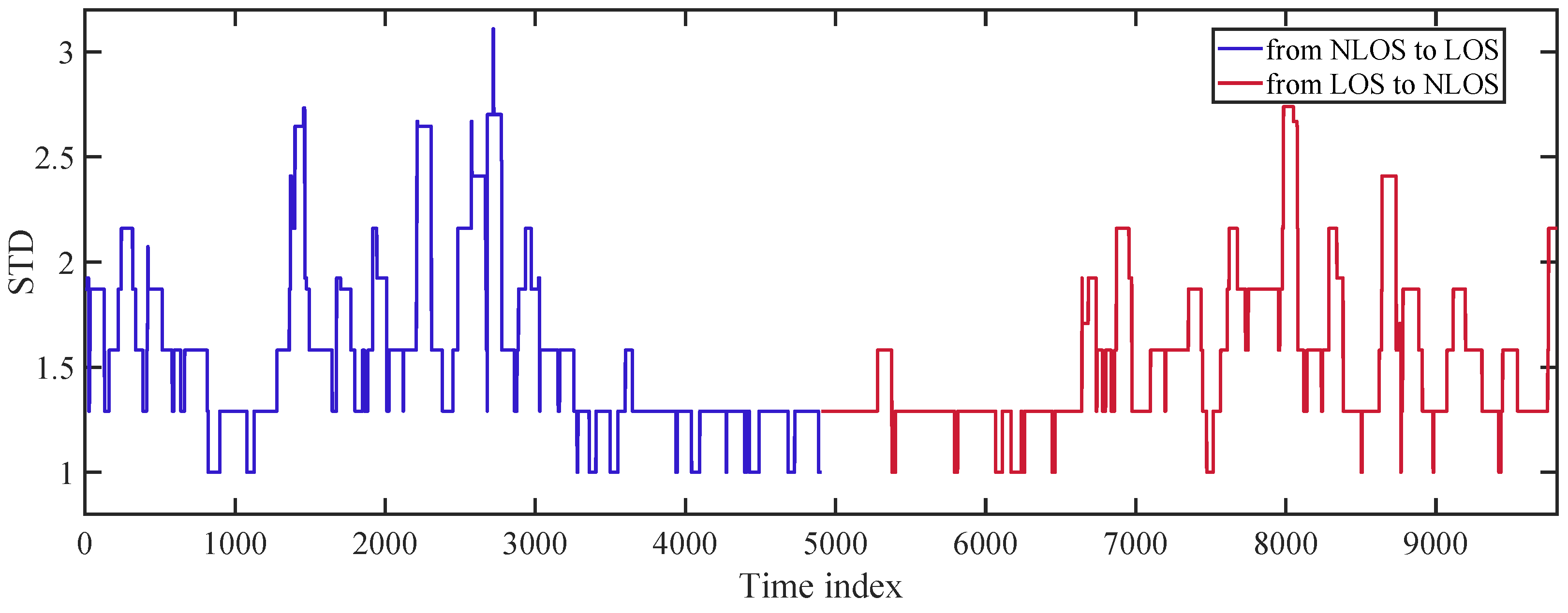
We collect two sets of data: one for walking out of the room (from LOS to NLOS) and the other for entering the room (from NLOS to LOS). Each lasts 10 s in total and contains 5000 packets. To verify the effectiveness of the selected feature, we calculate the STD of SIFPE during the time the user moves and plot the results in Figure 11. Since the window length is set to 95, we can obtain 4906 time indices for LOS/NLOS identification.

As shown in Figure 11, we present the concatenated curves of STD obtained from two consecutive experiments. The path status initially begins with NLOS, then transitions to LOS, and eventually returns to NLOS. It can be seen that the STD of NLOS paths is notably higher than that of LOS paths, enabling easy identification of the transition points between them. We can determine that the time point when the user enters the room lies between packet indices 3000 and 3200, while the time point when the user walks out of the room falls within the range of packet indices 6500 and 6700.

However, a significant challenge arises due to the presence of considerable noise in the calculated STD which can adversely impact the identification accuracy. To mitigate this issue, increasing the window length proves effective in reducing the impact of fluctuation and maintaining output stability. Nevertheless, it compromises the identification latency by extending the length of ambiguous outputs where LOS samples coexist with NLOS ones in the window.

5.4. Impact of Identification Delay

There are two sources of time delay for PEiD. One is the sampling time that happens in the initial step of the algorithm. The other is the transition time caused by channel state changes. The former can be ignored since it no longer occurs after the window is loaded. However, the latter can impact the performance of real-time LOS/NLOS identification. It counts because most packets remaining in the window belong to the NLOS path at the moment of LOS blocking. It takes time to update them with the new samples. When LOS samples coexist with NLOS ones in the window, the identification result of the model is ambiguous. Increasing the window length will lengthen the time of ambiguous results.

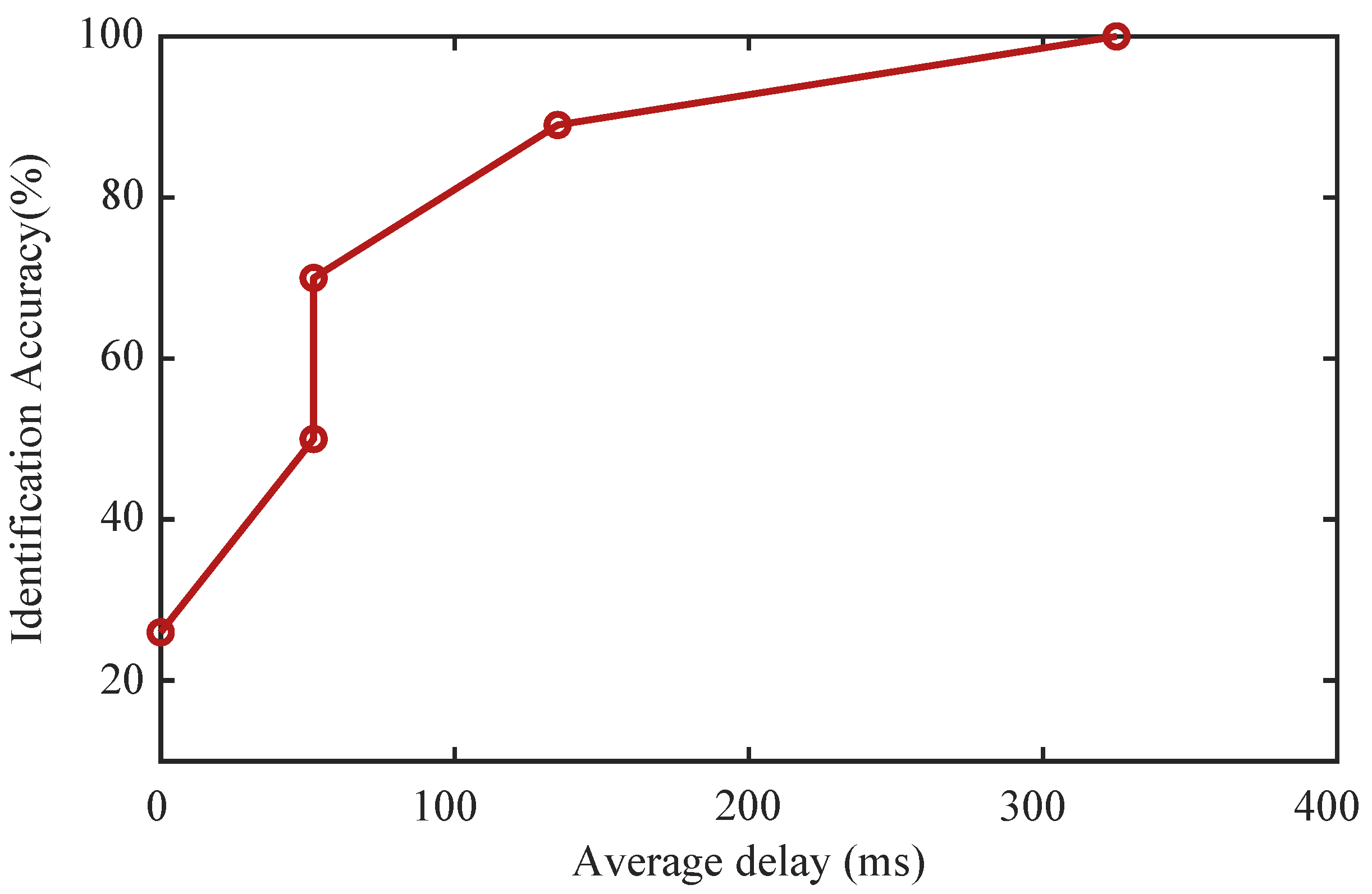
To confirm the impact of this problem on PEiD, we record the identification result at a fixed time after the channel state change. For each sample, the time of walking out of the room is regarded as the channel state transition point. Keeping the window length at 95, we test the performance with different time shifts and calculate the average identification accuracy. The results are shown in Figure 12.

The results depicted in Figure 12 reveal that the identification rate remains below 30% when the sampling time is short. However, as the delay surpasses 150 ms, the situation begins to improve. Specifically, when the delay is approximately 235 ms, corresponding to the average delay in a static situation, the identification accuracy can reach 95%. The complete identification of a sample requires a time delay of around 328 ms.

We believed such a latency is insignificant and acceptable for many in-home applications like gesture recognition and fall detection to determine the channel state. However, for applications with higher real-time requirements, such as trajectory tracking, our approach may still face challenges to maintain desired performance.

6. Conclusions

In this paper, we propose a machine-learning-based path identification approach called PEiD, which utilizes time domain features extracted from the commodity WiFi devices to achieve real-time and accurate LOS/NLOS classification. Our method explores a novel feature called peak energy index distribution that can effectively reflect the randomness of the channel property. Compared with previous works, PEiD can significantly reduce the sample size required for identification while maintaining a high performance. A sliding-window-based algorithm is also adopted to solve the problem of mobility. No manual operations or inertial sensors are needed in the process.

Nevertheless, our study also highlights two areas that require further improvement. Firstly, in indoor scenarios, the presence of rich multipath effects and environmental changes, such as different room layouts, can significantly impact channel properties. It is important to investigate whether the model trained in one environment can maintain its performance when confronted with a new scene. If the model’s performance degrades substantially and necessitates retraining, the challenge of collecting laborious samples arises. Future research should address this issue to ensure robust performance across diverse environments. Secondly, the features selected in our study are still limited. While we utilized CSI and CIR, there are numerous unexplored combinations and possibilities. With the advancements in deep learning, future work can explore the extraction of more complex features using kernel methods or neural networks. This approach can potentially uncover hidden patterns and enhance the accuracy and robustness of wireless sensing systems.

Overall, we believe that our work serves as a valuable supplement to existing methods for path identification. In the scenario of activity recognition, since our work can detect the blocking of direct paths, different data processing strategies can be made to eliminate discrepancies caused by channel state changes. In the scenario of user tracking that requires accurate localization at each time, our work can provide a real-time correction to the model when path status changes during the movement, ensuring precise trajectory estimation. PEiD achieves high path identification accuracy while maintaining a low identification delay, making it well-suited for practical applications.