Enhanced Evaluation Model Based on Classification Selection Applied to Value Evaluation of Waste Household Appliances

Abstract

In the process of recycling, dismantling, and reusing household appliances, implementing extended producer responsibility (EPR) has become increasingly important. Designing a reasonable pricing mechanism for waste household appliance recycling is critical for the implementation of EPR. To address the problem of labor-intensive and experience-dependent traditional manual methods for assessing the value of waste household appliances, in this paper, we propose an evaluation method based on the subtractive clustering method and an adaptive neuro fuzzy inference system (SCM–ANFIS), which outperforms traditional neural networks such as LSTM, BP neural network, random forest and Takagi–Sugeno fuzzy neural network (T–S FNN). Moreover, in this paper, we combine the five aforementioned algorithms to design a combination evaluation model based on maximum ratio combination (CEM–MRC), which can achieve a performance improvement of 0.1% in terms of mean absolute percentage error (MAPE) compared to the suboptimal BP neural network. Furthermore, an enhanced evaluation model based on classification selection (EEM–CS) is designed to automatically select the evaluation results between the optimal SCM–ANFIS and the suboptimal CEM–MRC, resulting in a 0.73% reduction in MAPE compared to the optimal SCM–ANFIS and a 1.42% reduction compared to the suboptimal CEM–MRC. In this paper, we also validate the performance of the proposed algorithms using a dataset of waste television recycling, which demonstrates the high accuracy of the proposed value assessment mechanisms achieved without human intervention and a significant improvement in evaluation accuracy as compared to conventional neural-network-based algorithms.

1. Introduction

Extended producer responsibility (EPR) refers to the practice whereby manufacturing companies are responsible not only for designing, producing, and selling products but also for their recycling, dismantling, and reuse. EPR is also an indispensable part of zero waste management [1]. By reducing the amount of waste products, EPR can promote the full utilization of resources and facilitate the development of a circular economy. In China, EPR has been applied to various manufacturing industries, such as household appliances [2], automobiles [3], and electronic products [4]. It is now extending to more industries under the encouragement of national policies. According to the UN’s 2020 Global E-waste Monitor Report, only 17.4% of the 53.6 million tons of global e-waste produced in 2019 were recycled [5]. EPR can effectively solve various social and environmental issues in e-waste recycling, such as handling heavy metals including lead, chromium, and mercury, in addition to addressing the problem of raw material shortages in manufacturing [6].

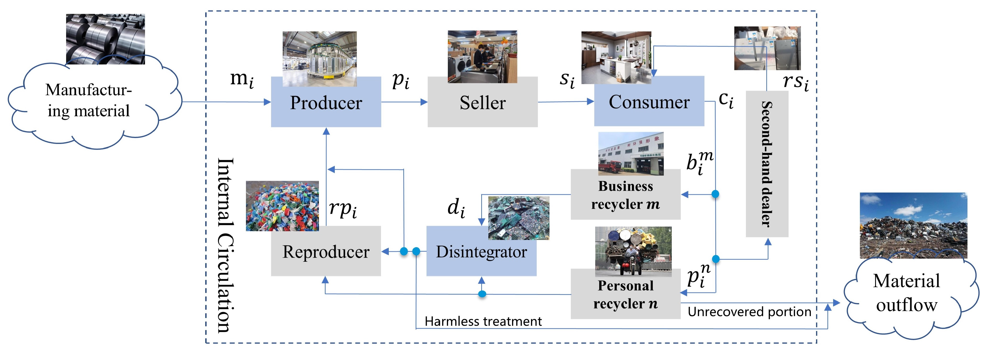
The main products involved in household appliance recycling are generally known as the “four appliances and one brain”, namely televisions, refrigerators, washing machines, air conditioners, and computers [7]. Figure 1 shows the material circulation process in the manufacturing and recycling of household appliances.

As shown in Figure 1, the industrial chain of household appliance recycling involves many participants, including producers, sellers, consumers, second-hand dealers, business recyclers, personal recyclers, disintegrators, and reproducers. Raw materials such as metal, plastic, and glass are sold to household appliance producers at a price of $m_i$. Producers sell household appliances to sellers at a factory price of $p_i$, and sellers sell them to consumers online or offline at a price of $s_i$. Since household appliances that are replaced by consumers may be sold to second-hand dealers or directly to scrap dealers, there are two circulation pathways for waste household appliances. One is to sell them to second-hand dealers at a price of $c_i$, then sell them to consumers at a price of $r{s}_i$. The second is to sell them to scrap dealers at a price of $c_i$. Scrap dealers can be divided into business recyclers and personal recyclers, and they are generally organized into multilevel networks according to their location. The selling price of the mth-level business recycler is denoted by $b_i^m$, and the selling price of the nth-level personal recycler is denoted by $p_i^n$. Personal recyclers usually do not have professional equipment, and they tend to dismantle waste household appliances privately, which not only exposes their employees to harmful substances and endangers their health [8] but also causes materials that cannot be recycled to flow out of the material circulation [9]. After dismantling, disintegrators sell the dismantled raw materials to reproducers at a price of $d_i$, and some materials that cannot be recycled are treated for harmless disposal, then flow out of material circulation [10]. Reproducers process the waste raw materials into reusable raw materials and sell them to household appliance producers at a price of $r{p}_i$, completing the internal circulation of materials in the manufacturing and recycling of household appliances. The pricing variables in the household appliance manufacturing and recycling process described above are summarized in

Table 1. Prices of materials at various stages of the manufacturing and recycling process.

Variable	Definition
$m_i$	The sum of the prices of all the raw materials needed in the process of appliance manufacturing (i)
$p_i$	The price at which a home appliance producer sells home appliance appliance i to a seller
$s_i$	The price at which a seller sells appliance i to a consumer
$c_i$	The price at which a consumer sells home appliance i to a second-hand dealer or recycler after use
$r{s}_i$	The price at which a second-hand dealer bring home appliance i back into the market through refurbishment [11] or repairing
$b_i^m$	The selling price of the m-th-level business recycler for household appliance i to the a next-level recycler
$p_i^n$	The selling price of the n-th-level personal recycler for household appliance i to a next-level recycler
$d_i$	The price of materials sold by a disintegrator to reproducers or home appliance producers after dismantling home appliance i
$r{p}_i$	The price of raw materials that reproducers sell to home appliance producers after reprocessing the recycled materials from home appliance i

.

Research on the household appliance recycling chain includes recycling techniques, pricing strategies based on game theory, market competition and cooperation models, etc. Bressanelli et al. [7] introduced the 4R strategy in the household appliance recycling circular economy, which includes reduction, reuse, remanufacturing, and recycling. Motoori et al. [11] proposed the full recycling of various metal materials in electronic products by increasing reuse rates and enhanced recycling efficiency. Cao et al. [12] constructed and analyzed a pricing strategy for recyclers based on a Stackelberg game model under EPR regulations, and the results showed that when the government is not the decision maker, the optimal product price of producers does not change under different strategies. They focused on three different closed-loop supply chain (CLSC) structures and different consumer categories. The authors of [13,14] studied competition and cooperation between producers and reproducers and investigated a circular game model of patents and carbon emissions. They discussed the impact of various policies and environmental factors on the decision making of supply chain system members. In China, there is a high production capacity for household appliances. Due to the longer lifespan of appliances and the rapid pace of product upgrades, the occurrence of reuse is relatively limited among Chinese consumers. As a result, the value assessment during the recycling process becomes even more critical, as the majority of waste household appliances are reprocessed through recycling methods. Although there is a growing emphasis on the replacement of old appliances with new ones in current policies, there is still a long way to go in terms of transitioning from the recycling stage to the reuse stage for waste household appliances. Therefore, conducting value assessment before the recycling process holds greater practical significance in terms of application and promotion. Consequently, the datasets used in our study specifically focus on the recycling scenario. During recycling, appliances are dismantled and crushed to recover materials, and the value of these materials remains relatively stable, making it feasible to obtain reasonably accurate estimates of material values.

However, there are still relatively few studies on the evaluation of household appliance recycling. The evaluation of each stage in the recycling chain is of considerable significance. For example, it helps to formulate reasonable pricing strategies, ensuring the profitability of recycling enterprises and providing more fair and reasonable prices for consumers. Moreover, it is helpful to find potential optimization space, such as by exploring more efficient recycling methods, reducing recycling costs, and improving recycling efficiency, thereby enhancing the efficiency of the entire recycling chain. Accurate evaluation methods are also beneficial for the discovery of potential economic benefits during the recycling process, attracting more enterprises and personnel to participate in recycling activities and promoting the effective recovery and utilization of resources. Johansson et al. compiled five short articles that focus on value assessment and pricing capabilities, bridging the gap between marketing, pricing, and strategic research [15]. Han et al. [16] proposed a fuzzy neural network-based evaluation model for the problem of accurate pricing in the process of recycling waste mobile phones. However, this model cannot be effectively applied to household appliance recycling due to differences in recycling mechanisms between mobile phones and household appliances. Wang et al. [17] proposed an attribute classification modeling method for electronic product evaluation. This method divides the attributes of electronic products into standard value, basic value, and depreciation value. However, the article did not provide a calculation method for the classified values. Sahan et al. [18] estimated components of recyclable precious metals and rare-earth elements from waste mobile phones in Turkey, but they did not apply the estimated results to recycling appraisal. No effective evaluation method for waste household appliance recycling has been proposed in the literature because the evaluation of household appliance recycling has unique characteristics and should be focused on waste raw materials as the main evaluation factor and combined with market game modeling to price the entire recycling chain. The most important entry point is the valuation of waste household appliances in the hands of consumers flowing into the recycling market, which is the most important part of the entire evaluation process in the recycling chain [19]. Machine learning methods have not yet been introduced for the evaluation of recycled waste household appliances.

The traditional method of evaluating waste household appliances is usually based on manual experience and rules. As a comparison, machine learning methods can adaptively learn and process new data and continuously improve prediction accuracy. Moreover, machine learning can process a large amount of data, optimize algorithms, and improve the accuracy as and speed of waste household appliance valuation while enabling intelligent decision making in support of the recycling industry. In this paper, we focus on value assessment for waste household appliances (i.e., the $c_i$ data in Figure 1) and propose a machine-learning-based evaluation model for recycling waste household appliances. The three main contributions of this paper are as follows:

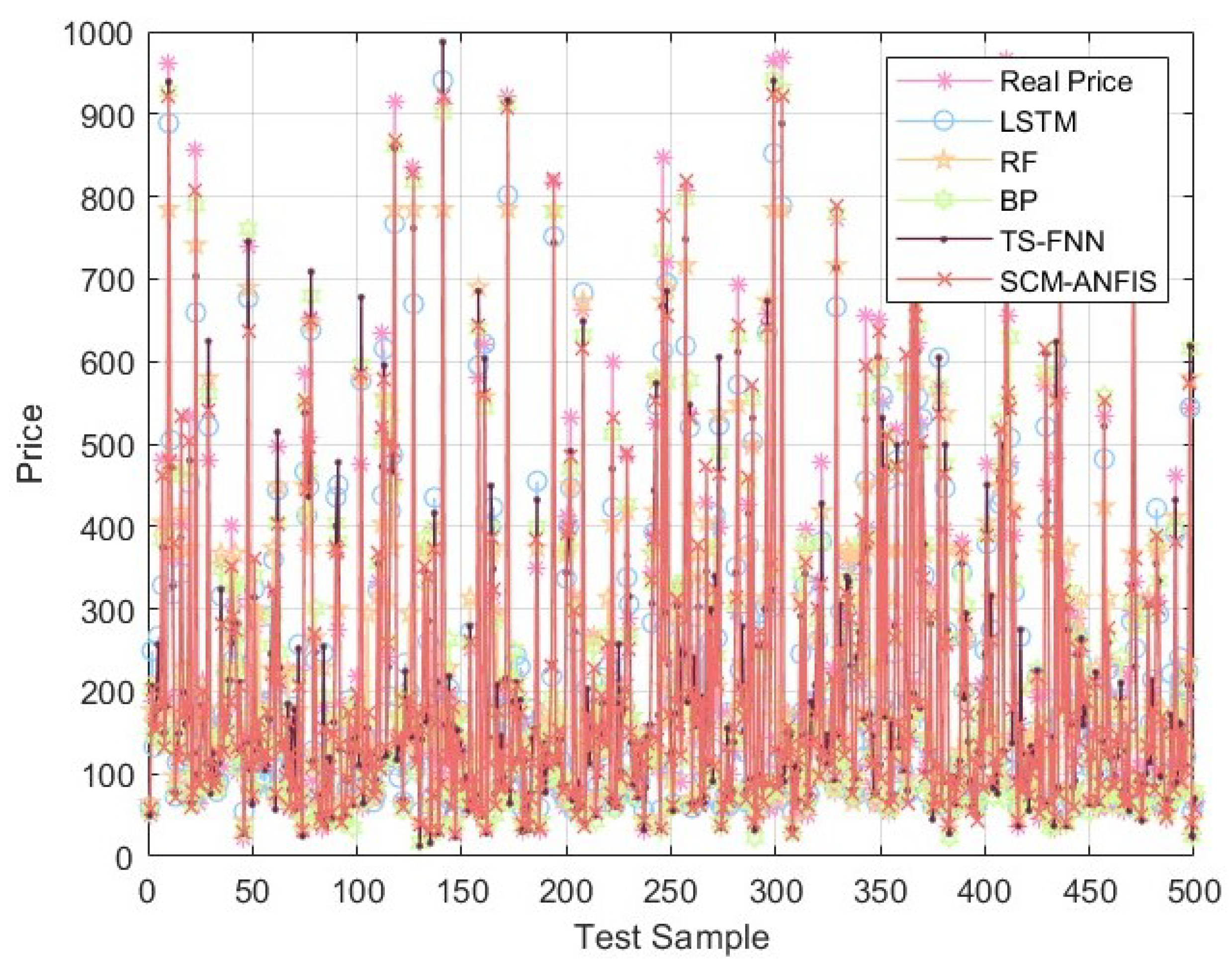
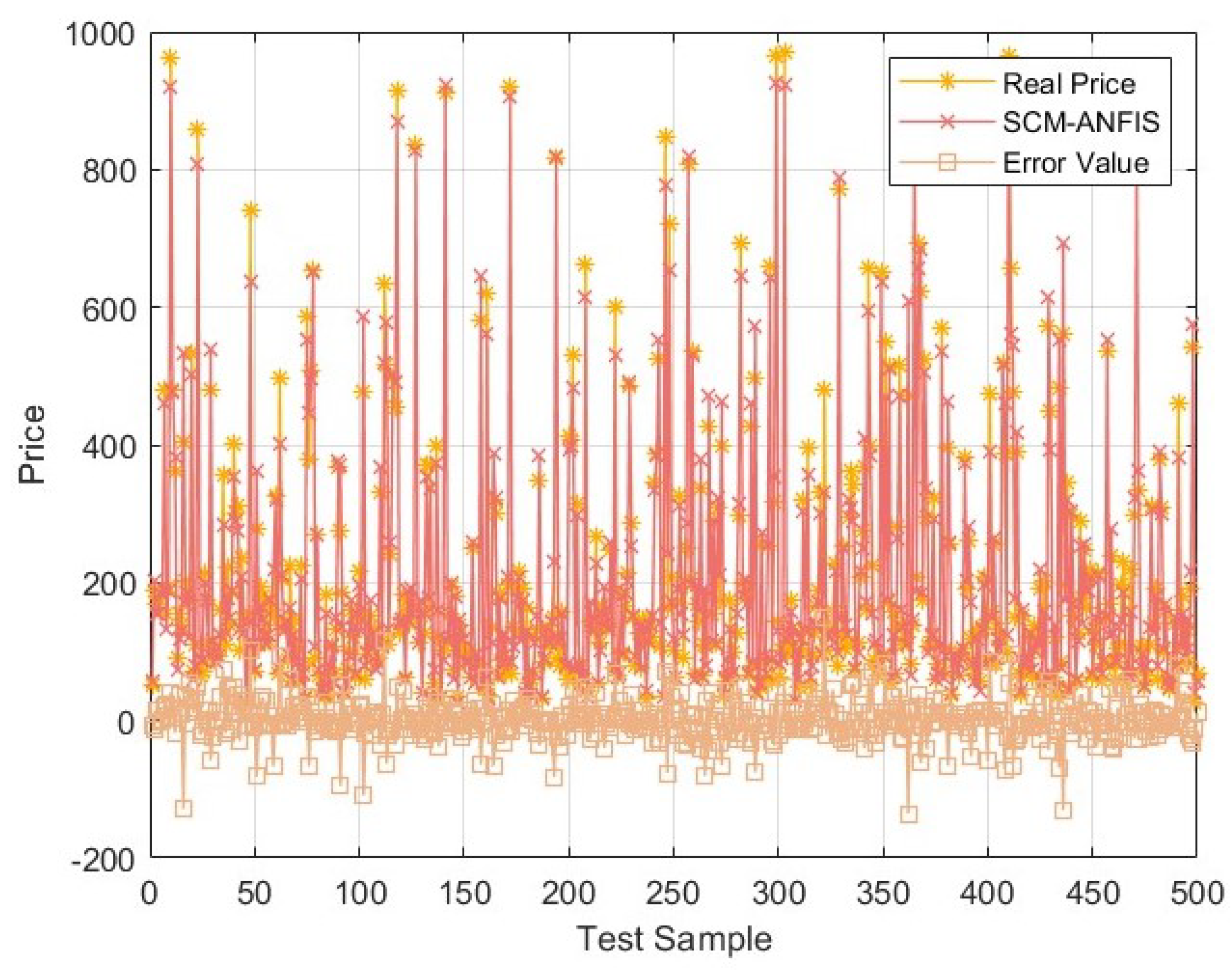
• A subtractive clustering method and adaptive network fuzzy inference system (SCM–ANFIS)-based evaluation algorithm is used to evaluate the waste TELEVISION dataset, achieving better results in terms of mean absolute percentage error (MAPE) than long short-term memory (LSTM), BP neural network, random forest (RF), and Takagi–Sugeno fuzzy neural network (T–S FNN);
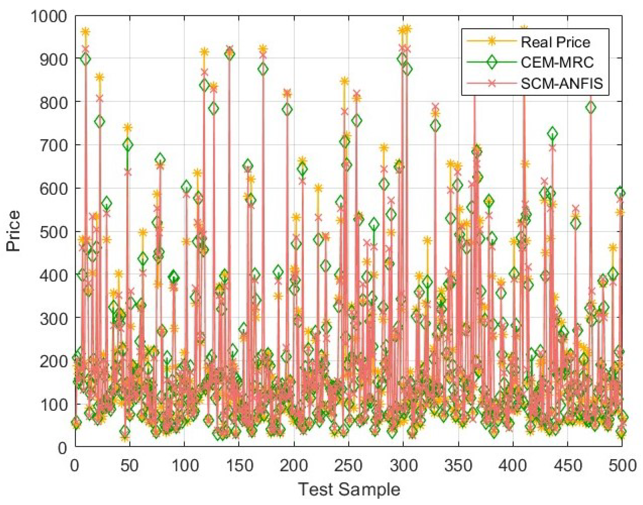
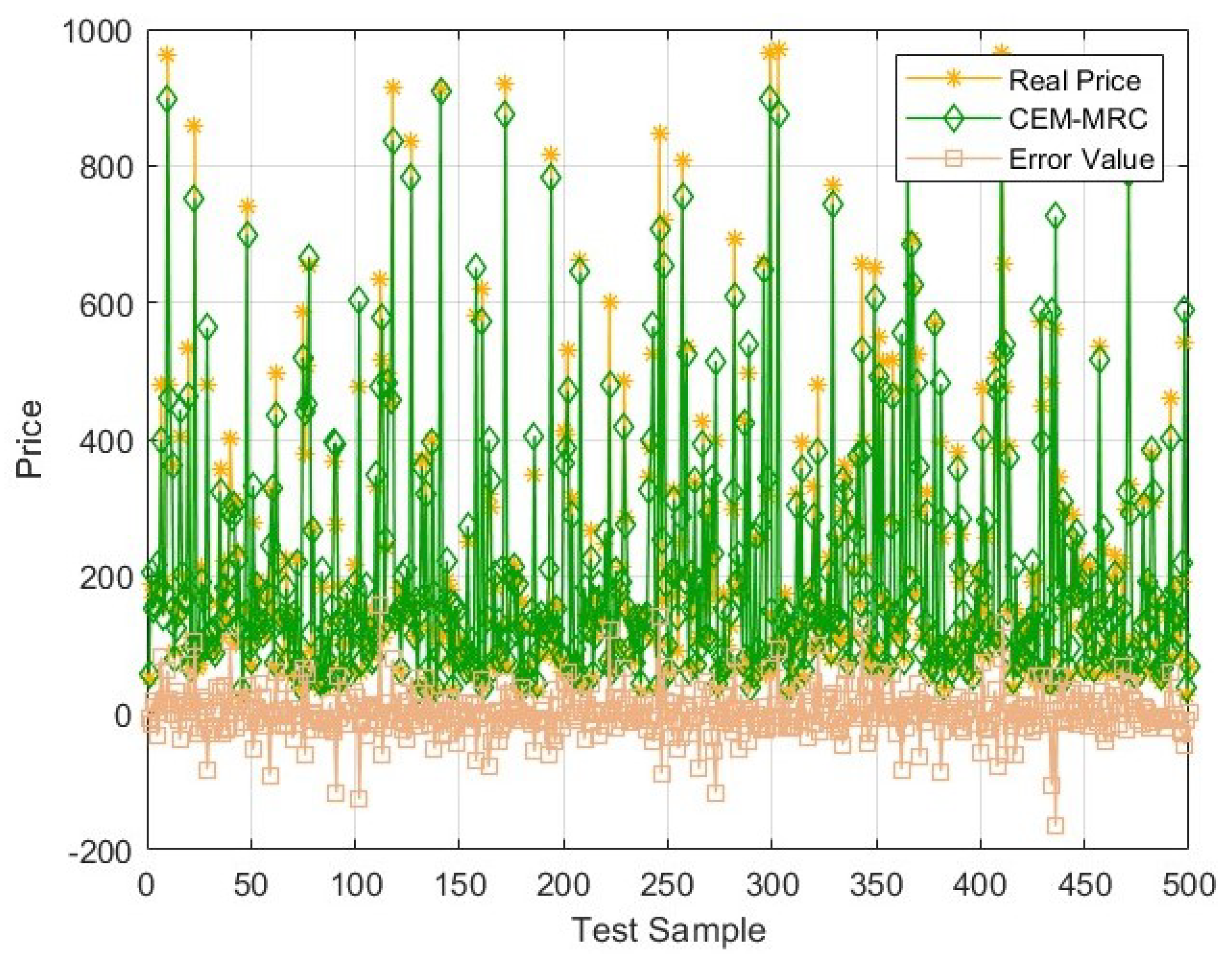
• A combination evaluation model based on maximum ratio combination (CEM–MRC) is constructed based on the machine learning methods mentioned above and compared with different combination methods to predict results. The results show that the maximum ratio combination method achieves the best performance among tested combination methods, with a lower MAPE than the suboptimal BP method, reducing it by 0.1%;
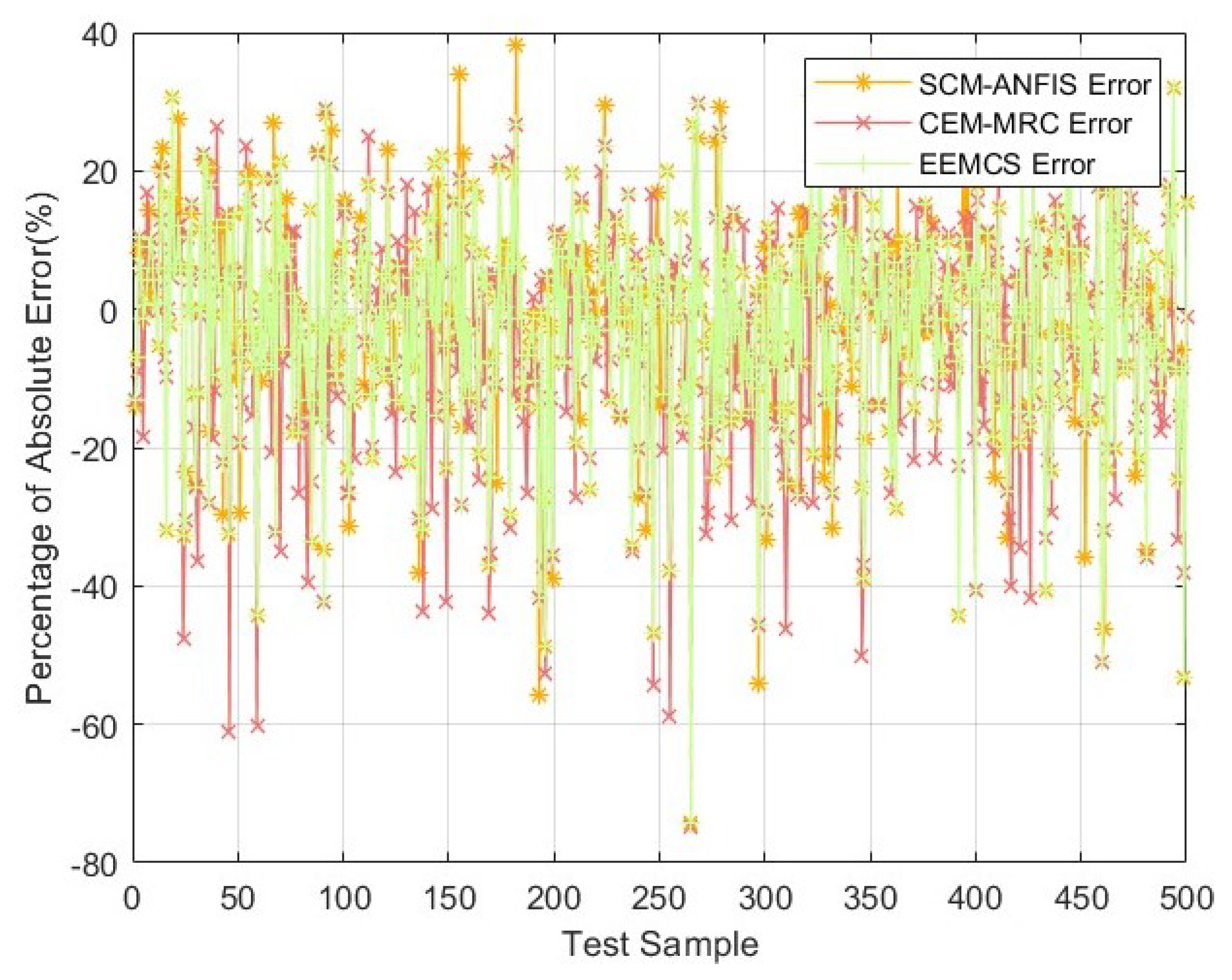
• An enhanced evaluation model based on classification selection (EEM–CS) is designed by combining the prediction models of CEM–MRC and SCM–ANFIS, which automatically selects the evaluation results between them. This method reduces the MAPE by 0.73% compared to the optimal SCM–ANFIS method and by 1.42% compared to the suboptimal CEM–MRC method on the training set.

The remainder of this paper is organized as follows. The second section provides an overview of the relevant technologies and their application in this research. The third section presents the framework for evaluating waste household appliances, elaborating on the algorithms and technical approach of the proposed model. In the fourth section, the evaluation results are presented, along with comparisons with different models, while the fifth section concludes the paper and provides future research directions.

2. Related Work

2.1. Adaptive Neuro Fuzzy Inference System

ANFIS is an adaptive system that combines the fuzzy inference capabilities of the Takagi–Sugeno model with the parameter-learning capabilities of neural networks. It uses neural networks to implement fuzzification, fuzzy inference, and defuzzification in fuzzy control by automatically extracting rules from input–output sample data and reasoning between fuzzy inputs and fuzzy outputs. Through learning and optimization processes, it improves the accuracy and generalization ability of the model and achieves automatic adjustment of fuzzy inference control rules.

Table 2. Comparison of neural networks, fuzzy logic system, and ANFIS technology.

Technology	Neural Networks	Fuzzy Logic	ANFIS
Basic Component	Neurons	Expert knowledge and rules	Neurons and Fuzzy Inference Units
Knowledge Acquisition	Samples and algorithm examples	Logical reasoning	Samples and expert knowledge
Inference Operation	Connection of neurons	Combination of fuzzy rules and heuristic search [17]	Membership functions and fuzzy inference
Representation	Distributed representation	Membership function	Membership functions and weight coefficients
Inference Effect	Weighted sum of neurons [16]	Max–min of membership function	Weighted sum of membership functions and weight coefficients
Adaptive	Learning by adjusting weights, high fault tolerance, and strong generalization ability	Inductive learning and low error tolerance	Adaptive hybrid of learning and fuzzy inference with high fault tolerance [20]
Advantages	Self-learning self-organization ability, high fault tolerance, strong generalization ability	Expert experience can be used, with high accuracy and interpretability	Combining the advantages of neural networks and fuzzy logic systems, it can not only deal with fuzzy problems but also learn adaptively
Disadvantage	Black box model, difficult to express knowledge, and difficult to understand and explain	The reasoning process is highly ambiguous, the learning and reasoning process is difficult, and the fault tolerance is relatively low [21]	The learning and fuzzy reasoning process is complex and requires considerable computing resources
Application Scenario	Pattern recognition, classification, prediction, and other problems that require high generalization ability	Deals with problems with high ambiguity, uncertainty, and complexity, such as control systems, decision support systems, and intelligent transportation systems	Can be applied in various fields, such as prediction, control, and classification

shows a comparison of neural networks, fuzzy logic systems, and ANFIS techniques, providing a clearer understanding of their similarities and differences.

ANFIS has been applied in various fields, such as system control [22], pattern recognition [23], data mining [24], medical biology [25], and regression prediction [26]. However, there has been no precedent for the use of an ANFIS network for value assessment in home appliance recycling. The advantage of neural networks lies in their ability to self-learn and self-organize, as well as their generalization ability, enabling them to learn and process input data by adjusting their weights. However, an ANFIS network is also a “black box model”, making it difficult to express and understand human knowledge. On the other hand, fuzzy logic systems can use expert experience for reasoning, but they have difficulty in learning, and the reasoning process may be vague. ANFIS combines the advantages of the above two approaches. In the evaluation of waste household appliances, owing to the ambiguity of the expressions of various attributes of waste household appliances, such as new, relatively new, super old, very damaged, etc., the use of fuzzy networks is suitable to handle fuzzy language.

2.2. Subtractive Clustering Method

Clustering is an unsupervised learning algorithm that learns data without labels. Therefore, the goal of unsupervised learning is to reveal the intrinsic properties and patterns of data by learning from unlabeled samples. Clustering partitioning metrics include density and distance [27], and there are many methods for distance partitioning, such as Euclidean distance, Manhattan distance, cosine distance, and Hamming distance. Subtractive clustering belongs is one type of density clustering [28], and the complexity of the clustering algorithm is generally linearly related to the dimensionality of the data.

ANFIS partitioning refers to the division of the input space into several subspaces and the modeling of each subspace using the same fuzzy rules. ANFIS input space is generally partitioned using one of two methods: grid partitioning (GP) or the subtractive clustering method (SCM) [29]. In the GP method, the input space is uniformly divided into a series of small grids, and each grid corresponds to a fuzzy rule. During the training process, the parameters of each rule (including membership functions and output functions) are adjusted to minimize the loss function. The advantage of grid partitioning is that it is easy to understand. However, when processing high-dimensional input spaces, the number of grids grows exponentially, leading to low training efficiency. When the number of input features exceeds 5, the computational cost becomes excessively high.

SCM is a distance-based clustering method, the main concept of which is to cluster based on the distances between input data. SCM first calculates the distance between each input sample, then aggregates the samples that are close in distance based on a threshold to obtain several clustering centers. ANFIS divides the input space into several subspaces based on these clustering centers and assigns corresponding fuzzy rules to each subspace. SCM can quickly obtain the clustering centers of data without the need to set the number of centers. Using SCM in ANFIS can solve the problem of high complexity and large numbers of rules in the pricing of recycled waste home appliances, reduce the number of generated rules, and lower the computational complexity of the algorithm, which is a direction that has not been fully explored.

3. Value Assessment Framework for Waste Household Appliances

In this section, we introduce the main factors influencing the value assessment of waste household appliances. Subsequently, the evaluation framework and data processing methods are presented using the case of waste televisions. Then, a detailed explanation of the steps involved in the SCM–ANFIS method, the CEM–MRC algorithm, and the EEM–CS algorithm are presented.

3.1. Key Factors in Value Assessment of Waste Home Appliances

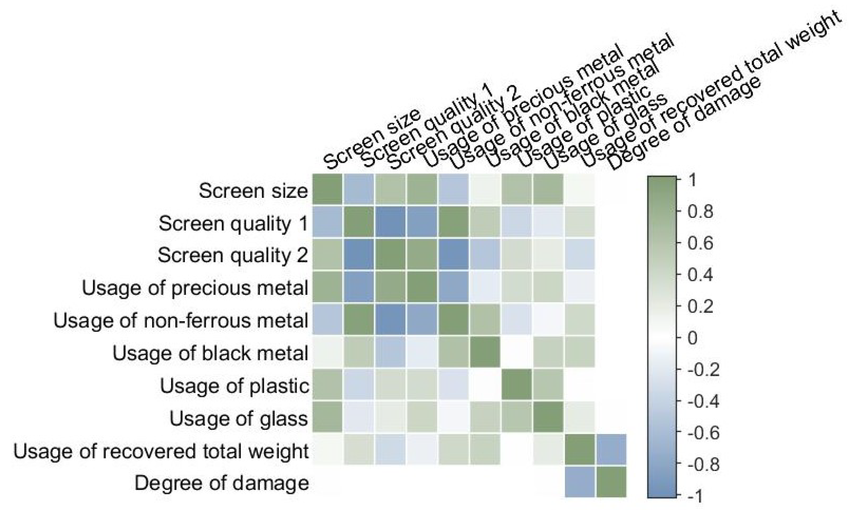
The methods for evaluating the value of waste household appliances are different from those used to evaluate recycled mobile phones or cars. Specifically, in the recycling of used mobile phones and cars, there is a large number of reusable components that can be repaired and refurbished before being reintroduced to the market. The main factors affecting the recycling price of these products are the model, usage time, and component parameters. However, waste household appliances have been used by users for a long time and are often considered outdated and undesirable. As a result, the recycling of these appliances mainly focuses on the recovery of raw materials such as metals (copper, steel, aluminum, etc.), glass, plastic, and paper. Waste household appliances are generally heavy, with a large proportion of metal materials. The pricing of waste household appliances for recycling is largely dependent on their weight, as well as other auxiliary factors, such as the brand of the appliance, usage time, damage level, screen type and condition, and the contents of various materials.

Therefore, it is necessary to propose effective algorithms for evaluation of recycled waste household appliances. In this paper, we take television recycling as an example to conduct an in-depth study on machine learning and fuzzy neural network algorithms for the evaluation of waste household appliances. Based on real market data on television recycling in China, a dataset of 6000 television recycling prices was expanded for evaluation.

3.2. Value Assessment Framework for TELEVISION Scrap

In order to achieve accurate valuation of waste televisions, we propose a reinforcement prediction model called EEM–CS with a classification selection mechanism, as shown in Figure 2. The main idea of this algorithm is to utilize different machine learning methods to evaluate the value of waste household appliances. Through iterative classification prediction training, the algorithm is able to select the optimal evaluation result as the final output value assessment.

The design architecture mainly consists of three modules: data preprocessing, model training, and evaluated price output. The functions of each module are described below.

3.2.1. Data Preprocessing

The data preprocessing module includes abnormal data processing, one-hot encoding, data diversity, and normalization submodules, as described below.

• Abnormal data processing: For the dataset of 6000 waste television recycling data entries, outlier and noise data are handled using methods such as the 3-sigma rule, Boxplot, Z-score, and Grubbs. Outlier data can be deleted, while missing data can be supplemented using the mean.
• One-hot encoding: Since the dataset involves characteristics such as television brand and screen quality that cannot be recognized directly by neural networks, they need to be encoded as numerical data. One-hot encoding is used as an effective encoding method. Assuming there are M states to be encoded, the number of bits in one-hot encoding is M, and only one bit is 1, while the rest are 0. For example, there are two states in the case of screen quality in waste home appliances: good or bad. The code for good screen quality can be represented by “01”, while the code for bad screen quality can be represented by “10”. After all text information is one-hot-encoded, it is concatenated with the original data to form a new dataset.
• Data diversity and normalization: The 6000 encoded data entries are randomly divided into a training set and a test set in a ratio of 11:1. Both the training and test sets are standardized to eliminate numerical problems caused by different dimensions and scales of data [30]. In this paper, we adopt the MinMax normalization method, which scales the original data to the interval [0, 1]. Let $x_1$, $x_2$, …$x_j$, …$x_n$ be the data, where $x_{max}$ represents the maximum datum, and $x_{min}$ represents the minimum datum. The processed new data ($x_j^{\prime }$) of the original data ($x_j$) are represented by:

  $${\mathsf{\Delta }}_j=x_{max}-x_{min}$$

  (1)

  $$x_j^{\prime }=(x_j-x_{min})/{\mathsf{\Delta }}_j$$

  (2)

3.2.2. Model Training

The model-training module includes PCA dimensionality reduction and model-training submodules, as follows:

• PCA dimensionality reduction: Principal component analysis (PCA) is a detection method based on multivariate statistical analysis, which is usually used for feature extraction and data dimensionality reduction in machine learning [31]. PCA can represent data using fewer principal components without losing too much information, thus reducing the dimensionality of the data [32].
    After normalizing the indicator data, the training set (X), which has p feature factors and n samples, is represented as follows:

  $$X=[X_1,X_2,\dots ,X_i,\dots ,X_p]$$

  (3)

  $$X_i={[x_{i1},x_{i2},\dots ,x_{ij},\dots ,x_{in}]}^T$$

  (4)
    Next, the matrix (Z) is calculated. Z is obtained by standardizing the matrix operation on X, and the correlation coefficient matrix R is obtained as follows:

  $$R=\frac{1}{n-1}{Z}^{T}Z$$

  (5)
    Then, we solve the unknown variable ($\lambda$) in the characteristic equation ($|R-\lambda I_k|=0$) of the correlation matrix (R) and obtain p eigenvalues:

  $$\{{\lambda }_1,\dots ,{\lambda }_j,\dots ,{\lambda }_p\}$$

  (6)

  $$Y_j=\frac{{\lambda }_j}{{\sum }_{j=1}^p{\lambda }_j}$$

  (7)
    The value of $Y_j$ is calculated and represents the contribution rate of the $jth$ principal component. The magnitude of the contribution rate reflects the amount of information contained in $X=[X_1,X_2,\dots ,X_i,\dots ,X_p]$.

  $$C=\frac{{\sum }_{j=1}^m{\lambda }_j}{{\sum }_{j=1}^p{\lambda }_j}$$

  (8)
    Then, the cumulative contribution rate (C) of the eigenvalues can be calculated. Generally, if m feature factors are selected for dimension reduction, m is chosen such that the cumulative contribution rate (C) is greater than 0.85, indicating that these m indicators can already represent the major information related to X [16]. In this paper, feature factors with a C value greater than 0.9 are selected as the primary input.
• Model Training
    After PCA dimensionality reduction, the data are trained using five models: SCM–ANFIS, BP, T–S FNN, RF, and LSTM. The output result of the SCM–ANFIS model is denoted as $pric{e}_1$. A BP neural network is a multilayer feed-forward neural network, and its learning algorithm uses backpropagation to update the network weights. T–S FNN is a type of neural network based on fuzzy logic, and each output of T–S FNN is composed of a set of linear functions. T–S FNN maps the input variables to membership functions, then uses fuzzy rules for inference and weights each output of each rule. RF uses randomly selected subsets of training data and feature subsets to train each decision tree to increase the randomness of the tree. RF determines the final output by voting for each decision tree. LSTM is a special type of recurrent neural network used to handle sequence data with long-term dependencies. The state unit in LSTM can store long-term information, while the hidden state can pass short-term information [33].
    The training set uses 5500 sets of data, and we save the trained model and input it into the evaluation module. The output prices of the above five models are denoted as $pric{e}_a$, $pric{e}_b$, $pric{e}_c$, $pric{e}_d$, and $pric{e}_e$.

3.2.3. Value Evaluation Module

We propose two algorithms for the evaluation module, namely CEM–MRC and EEM–CS. CEM–MRC utilizes the maximum ratio combination algorithm to weightedly combine the five evaluation prices ($pric{e}_a$, $pric{e}_b$, $pric{e}_c$, $pric{e}_d$, and $pric{e}_e$) to obtain an evaluation result that comprehensively incorporates the advantages of various methods. On the other hand, EEM–CS employs supervised learning after the addition of labels to enable the model to output the optimal evaluation result between SCM–ANFIS and CEM–MRC.

• CEM–MRC
    The output results of the training set data of the above five models are calculated using the maximum ratio combination method to obtain the weights of different models. The weights are then used to obtain the output result of the CEM–MRC method in the test set (denoted as $pric{e}_2$) through weighted combination.
• EEM–CS
    We use the maximum ratio combination method on the training set to construct auxiliary reference price variables, i.e., using $pric{e}_1$ and $pric{e}_2$ to construct the estimated true price ($pric{e}_3$). The three prices and the dataset after PCA dimensionality reduction are used as the output of the training set and sent to the EEM–CS prediction model for training. In the training set, we mark which method obtains the lowest MAPE between SCM–ANFIS and CEM–MRC as the classification basis. After training the classification model with the above data, the model can evaluate which method should be chosen for value assessment of an arbitrary test datum. Finally, the EEM–CS method selects either the SCM–ANFIS or CEM–MRC method to output the final evaluation results of the waste household appliances in the test set.

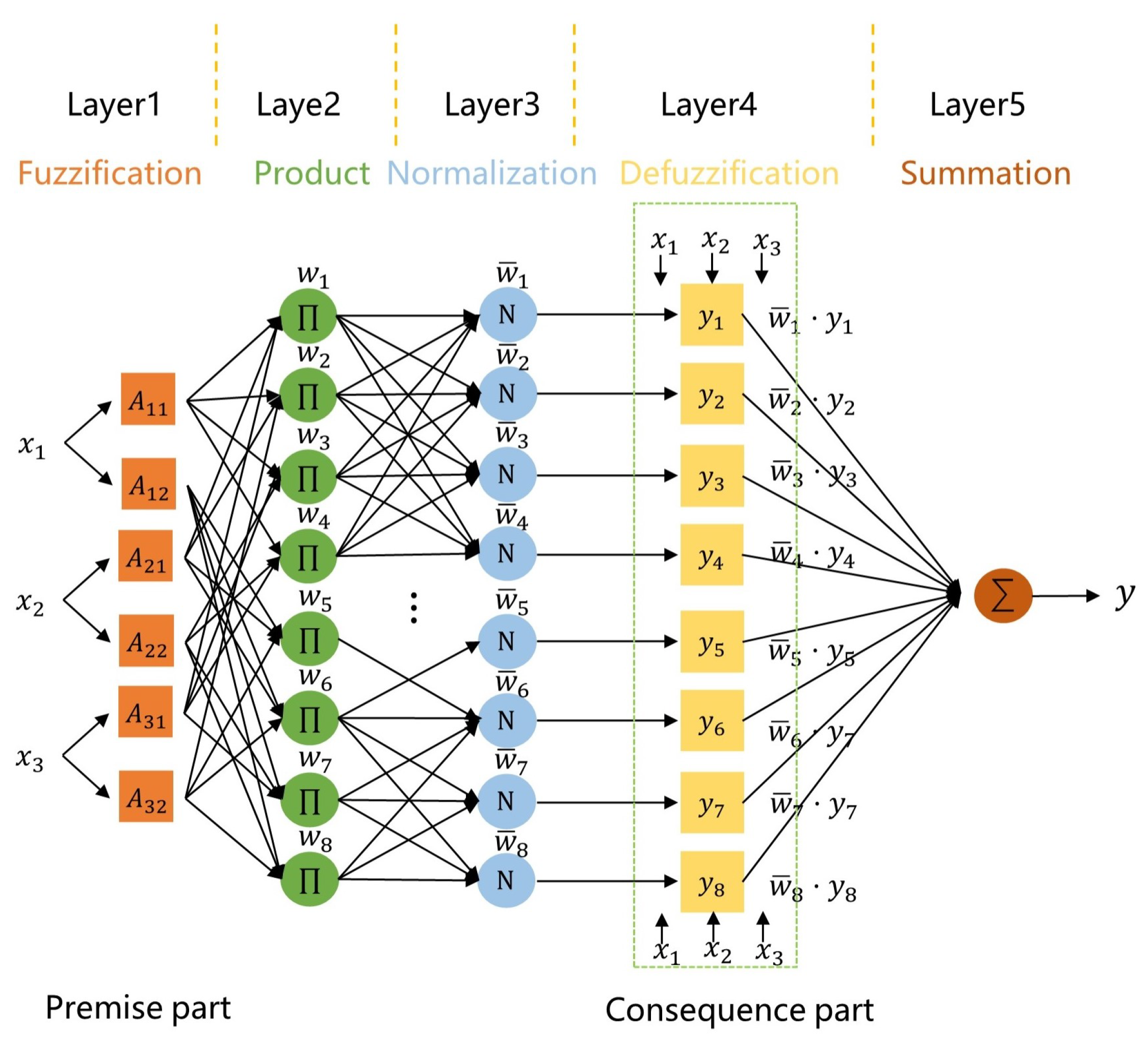
3.3. SCM–ANFIS Algorithm Design

In this section, we present the details of the proposed SCM–ANFIS. Similar to T–S fuzzy neural networks, ANFIS also uses if–then rules. Each rule consists of an antecedent (if) and consequent (then) parts. The antecedent specifies the fuzzy conditions based on the input variables, and the consequent part specifies the fuzzy conclusion based on the output variable. Let $R^p$ denote a fuzzy rule, where p indicated the number of rules. The expression of the rule is as follows:

$$R^p:if{x}_{1}is{A}_{p1}and{x}_{2}is{A}_{p2}and\dots and{x}_{k}is{A}_{pk},then{y}_p=c_{p0}+c_{p1}{x}_1+c_{p2}{x}_2+\cdots +c_{pk}{x}_k$$

Here, the “if” part is fuzzy and is called the antecedent or premise. $x_1,x_2,\dots ,x_k$ represent the input system variables, and $A_{p1},A_{p2},\dots ,A_{pk}$ represent the corresponding fuzzy sets. The “then” part is determinate and is called the consequent or inference part. y represents the inference result (e.g., estimated value), and $c_{p0},c_{p1},\dots ,c_{pk}$ represent different weights of input variables. Figure 3 illustrates a three-input–one-output ANFIS structure. The input represents the input variables required for the valuation of waste home appliances, such as appliance specifications, brand, weight, etc. Each input variable is typically represented by a set of fuzzy sets, which are used to capture the degree of fuzziness or membership of the input variables. The fuzzification layer converts the input variables from their actual values into membership degrees within the fuzzy sets. The product layer consists of a set of fuzzy rules. The condition part of each rule matches the membership degrees of the input variables, and an activation level is assigned to each rule, indicating the degree or weight of the rule. The normalization layer combines the activation levels of the fuzzy rules with the membership functions of the rules to calculate the matching degree of each rule. The defuzzification layer combines the activation levels of all rules to generate the aggregated fuzzy output. The summation layer converts the aggregated fuzzy output into concrete values or fuzzy sets, representing the final evaluation result.

Before we input the data samples into the ANFIS network, they should be clustered to reduce the number of potential rules that will be generated, as shown in the following. Assuming n data samples ($X_i={[x_1,x_2,\dots ,x_i,\dots ,x_n]}^T$) in the training set, each data point ($x_i$) is a potential cluster center, and the density ($D_i$) of each data point is calculated first.

$$D_i={\sum }_{j=1}^{n}exp\left(\frac{-\left|\right|x_i-x_j{\left|\right|}^2}{{\left(\frac{r_a}{2}\right)}^2}\right)$$

(9)

$$D_i=4{\sum }_{j=1}^{n}exp\left(\frac{-\left|\right|x_i-x_j{\left|\right|}^2}{{\left(r_a\right)}^2}\right)$$

(10)

where $r_a$ represents the radius of clustering. A large number of data points within the radius indicates that the density of the data point is high. The clustering algorithm selects the data point with the highest density as the center. When calculating the density of other data points, the influence of the selected cluster centers needs to be removed. Let $x_i$ be the selected data point and $D_c$ be its density. Then, Formula (10) is modified as follows:

$$D_i=D_i-4D_c{\sum }_{j=1}^{n}exp\left(\frac{-\left|\right|x_i-x_c{\left|\right|}^2}{{\left(r_b\right)}^2}\right)$$

(11)

where $r_b$ represents the radius with obvious decreased density, indicating that the density of the data points near the first cluster center ($x_c$) decreases after modification and that they are unlikely to become the next cluster center. The above steps are repeated to select the next cluster center until the desired number of cluster centers is obtained [34].

3.4. CEM–MRC Algorithm Design

We propose three main principles for CEM–MRC: the reverse combination method, the direct combination method, and the maximum ratio combination method. The difference between these methods lies in the weighting method used for different machine learning methods during the weighting process.

3.4.1. Inverse Combination Method

Suppose that the MAPE of different training models (i.e., SCM–ANFIS, BP, T–S FNN, RF, and LSTM) on the training set is ${\vartheta }_1,{\vartheta }_2,\dots ,{\vartheta }_i,\dots ,{\vartheta }_5$ and that the corresponding combination weight ($w_i$) is

$$w_i=\frac{1/{\vartheta }_i}{{\sum }_{i=1}^{N}1/{\vartheta }_n},i=1,2,\dots ,5.$$

(12)

The output value of the inverse combination method is

$$p={\sum }_{i=1}^N{w}_i{p}_i$$

(13)

where $p_1,p_2,\dots ,p_i,\dots ,p_5$ represent the evaluation prices of different models. A lower MAPE of a specific model indicates that a smaller error can be achieved, and, hence, the weight of that model should be larger.

3.4.2. Exponential Combination Method

Suppose that the MAPE of different training models( i.e.,SCM–ANFIS, BP, T–S FNN, RF, and LSTM) on the training set is ${\vartheta }_1,{\vartheta }_2,\dots ,{\vartheta }_i,\dots ,{\vartheta }_5$ and that the combination weight ($w_i$) can be expressed as

$$w_i=\frac{e^{-{\vartheta }_i}}{{\sum }_{i=1}^N{e}^{-{\vartheta }_n}},i=1,2,\dots ,5.$$

(14)

The output value of the exponential combination method is

$$p={\sum }_{i=1}^N{w}_i{p}_i$$

(15)

where $p_1,p_2,\dots ,p_i,\dots ,p_5$ represent the evaluation prices of different models. This method has is advantageous because it has a lower MAPE as compare to the inverse combination method.

3.4.3. Maximum Ratio Combination Method

The maximum ratio combination (MRC) method is different from the two combination methods mentioned above. It adopts the idea of maximizing the signal-to-noise ratio from communication and is therefore an optimal solution.

Let $X_{est1},X_{est2},X_{est3},X_{est4},X_{est5}$ be the output results of different training models for 5500 data samples in the training set, as represented by column vectors. $X_{ACC}$ represents the true price of the training set, and $N_1,N_2,N_3,N_4,N_5$ represent the errors between the predicted values and the true values.

$$\begin{array}{c}\hfill X_{est1}=X_{ACC}+N_1\\ \hfill X_{est2}=X_{ACC}+N_2\\ \hfill X_{est3}=X_{ACC}+N_3\\ \hfill X_{est4}=X_{ACC}+N_4\\ \hfill X_{est5}=X_{ACC}+N_5\end{array}$$

(16)

Let Y be the aggregated matrix composed of the output results of different training models on the training set; then,

$$Y=\left(\begin{array}{c}{X}_{est1}^T\\ X_{est2}^T\\ X_{est3}^T\\ X_{est4}^T\\ X_{est5}^T\end{array}\right)=\left(\begin{array}{c}1\\ 1\\ 1\\ 1\\ 1\end{array}\right)X_{ACC}^T+\left(\begin{array}{c}{N}_1^T\\ N_2^T\\ N_3^T\\ N_4^T\\ N_5^T\end{array}\right)$$

(17)

$$H=\left(\begin{array}{c}1\\ 1\\ 1\\ 1\\ 1\end{array}\right),N=\left(\begin{array}{c}{N}_1^T\\ N_2^T\\ N_3^T\\ N_4^T\\ N_5^T\end{array}\right)$$

(18)

Let $W=\left(\begin{array}{ccccc}{w}_1& w_2& w_3& w_4& w_5\end{array}\right)$ represent the weights of different models, where $w_i$ is scalar. Then,

$$\begin{array}{cc}\hfill WY& =\left(\begin{array}{ccccc}{w}_1& w_2& w_3& w_4& w_5\end{array}\right)\left(\begin{array}{c}{X}_{est1}^T\\ X_{est2}^T\\ X_{est3}^T\\ X_{est4}^T\\ X_{est5}^T\end{array}\right)\hfill \\ \hfill & =w_1{X}_{est1}^T+w_2{X}_{est2}^T+w_3{X}_{est3}^T+w_4{X}_{est4}^T+w_5{X}_{est5}^T\hfill \end{array}$$

(19)

$$WY=WH{X}_{ACC}^T+WN$$

(20)

The signal-to-noise ratio (SNR) can then be expressed as:

$$SNR=\frac{WH{X}_{ACC}^T{X}_{ACC}{H}^T{W}^T}{WN{N}^T{W}^T}$$

(21)

To maximize SNR, $X_{ACC}^T$ is a known fixed value. Thus, $H{X}_{ACC}^T{X}_{ACC}{H}^T$ is a constant, and the above equation is equal to maximizing the following formula:

$$max\frac{WH{H}^T{W}^T}{WN{N}^T{W}^T}=\frac{{(w_1+w_2+w_3+w_4+w_5)}^2}{w_1^2{N}_1^T{N}_1+w_2^2{N}_2^T{N}_2+w_3^2{N}_3^T{N}_3+w_4^2{N}_4^T{N}_4+w_5^2{N}_5^T{N}_5}$$

(22)

As this is a weighted method, we have $w_1+w_2+w_3+w_4+w_5=1.$ To maximize the above Formula (22), the denominator needs to be minimized:

$$min\{w_1^2{N}_1^T{N}_1+w_2^2{N}_2^T{N}_2+w_3^2{N}_3^T{N}_3+w_4^2{N}_4^T{N}_4+w_5^2{N}_5^T{N}_5\}$$

(23)

Then, we obtain

$$w_1^2:w_2^2:w_3^2:w_4^2:w_5^2=\frac{1}{N_1^T{N}_1}:\frac{1}{N_2^T{N}_2}:\frac{1}{N_3^T{N}_3}:\frac{1}{N_4^T{N}_4}:\frac{1}{N_5^T{N}_5}$$

(24)

Finally, the maximum combined output value is

$$p={\sum }_{i=1}^N{w}_i{p}_i$$

(25)

3.5. EEM–CS Algorithm Design

Although the SCM–ANFIS method achieves better performance in terms of absolute error for 3003 datasets among the 5500 training sets, there are still nearly 40% of data samples for which the CEM–MRC method performs better. If specific scenarios can be identified with respect to when to use SCM–ANFIS and when to use CEM–MRC, then the MAPE in the testing set can be further improved. Motivated by this, we propose the EEM–CS method as shown in Figure 4, which combines SCM–ANFIS and CEM–MRC methods and uses the classification regression method of machine learning to set up supervised learning on the training set in order to achieve intelligent selection of SCM–ANFIS or CEM–MRC in the testing set. Specifically, we expect that the classification model can accurately select the algorithm that should be used for the testing set. To this end, we set labels for the data samples in the training set based on which algorithm can achieve a smaller error as compared to the real price. However, the exact value of the recycled TV scrap is usually not known in practice, so it cannot be input to the training set for training. To solve this difficulty, we propose the use of the maximum ratio-merging algorithm to construct an auxiliary variable, denoted as $X_{price3}$, from the estimation results of SCM–ANFIS and CEM–MRC, which is used to take the place of the real price of TV scrap as the input for the classification regression training algorithm. Algorithm 1 shows a flow chart of the proposed EEM–CS algorithm, which uses an RF algorithm to train the classification model and achieve the intelligent selection of evaluation algorithms.

Algorithm 1: EEM–CS algorithm description.

1: Carry out one-hot coding, convert text information into coded information, so as to adapt to computer calculation 2: Divide 6000 sets of data into 5500 sets as training sets and 500 sets as test sets 3: Perform data normalization to adapt to algorithmic perception 4: Carry out PCA principal component analysis, and select principal components with cumulative contribution >90% for value evaluation algorithm 5: Carry out training algorithm on the training sets based on SCM–ANFIS, BP neural network, LSMT, T–S FNN, and random forest model, and the training results are denoted as $[X_{est1}^{train},X_{est2}^{train},X_{est3}^{train},X_{est4}^{train},X_{est5}^{train}]$ 6: Calculate the weights of the different models using the maximum ratio combining algorithm, with $N_i$ represent the error between the estimated value and the actual value: $$N_i=X_{ACC}-X_{est1}^{train}$$ $$w_1^2:w_2^2:w_3^2:w_4^2:w_5^2=\frac{1}{N_1^T{N}_1}:\frac{1}{N_2^T{N}_2}:\frac{1}{N_3^T{N}_3}:\frac{1}{N_4^T{N}_4}:\frac{1}{N_5^T{N}_5}$$ $$\sum _{i=1}^{n=5}{w}_i=1$$ 7: The training results of the test sets are denoted as $[X_{est1}^{test},X_{est2}^{test},X_{est3}^{test},X_{est4}^{test},X_{est5}^{test}]$; calculate the maximum ratio and combine the output results of the training set $X_{MRC}^{train}={\sum }_{i=1}^{n=5}{w}_i{X}_{esti}^{train}$ and test set $X_{MRC}^{test}={\sum }_{i=1}^{n=5}{w}_i{X}_{esti}^{test}$ 8: Mark on each data sample in the training set by 1 or 2 based on whether $X_{MRC}^{train}$ or $X_{est1}^{train}$ has smaller error as compared to the true price respectively: $label=\left\{\begin{array}{c}\hfill 1,ifabs(x_{MRC}^{train}-x_{true}^{train})<abs(x_{MRC}^{train}-x_{test1}^{train})2,ifabs(x_{MRC}^{train}-x_{true}^{train})\ge abs(x_{MRC}^{train}-x_{est1}^{train})\end{array}\right.$ 9: Use the maximum ratio merging algorithm 5–6 to construct the auxiliary variable price $X_{price3}$, and insert the three data $X_{price3},X_{MRC}^{train},X_{est1}^{train}$ into the input data set of the classification model together 10: Use RF algorithm to train the classification model to realize the enhanced prediction of classification selection, automatically select $X_{MRC}^{test}$ or $X_{est1}^{test}$ in the test set, $X_{EEM-CS}^{test}=switch(X_{MRC}^{test},X_{est1}^{test})$, in order to achieve reduced MAPE

4. Results and Discussion

4.1. SCM–ANFIS

In the dataset of 6000 waste televisions, PCA was performed to select variables with a cumulative contribution rate greater than 90%. The original dataset contained 11 feature variables, including brand, display type, screen size, screen condition, precious metal usage, non-precious-metal usage, black metal usage, plastic usage, glass usage, and the corrected total weight of the recycled materials, as well as the damage level. Due to the brand variable containing data from nine different electronics producers, the number of bits used for it became extremely large after hot encoding, resulting in an exceptionally large computational load during machine learning training. Therefore, data dimensionality reduction is necessary.

Table 3. Contributions of different principal components.

Principal Component	Contribution (%)	Cumulative Contribution Rate (%)
Degree of damage	32.33%	32.33%
Usage of recovered total weight	11.99%	44.32%
Usage of glass	8.37%	52.69%
Usage of plastic	6.86%	59.55%
Usage of black metal	5.38%	64.93%
Usage of non-ferrous metal	5.37%	70.30%
Usage of precious metal	5.36%	75.65%
Screen size	5.35%	81.00%
Screen quality 1	5.34%	86.34%
Screen quality 2	5.33%	91.68%

and Figure 5 show the contributions of different principal components in PCA, indicating that the damage level accounts for a significant proportion in terms of feature contribution. Screen quality is scaled to two factors due to one-hot encoding. We selected these ten feature variables after PCA analysis as input parameters for evaluation of the value of waste household appliances and implemented subsequent training models.

The correlation coefficients between different principal components are shown in Figure 6. The correlation coefficient (${\rho }_{X,Y}$) is calculated using the following formula:

$${\rho }_{X,Y}=\frac{cov(X,Y)}{{\sigma }_X{\sigma }_Y}=\frac{E\left[(X-{\mu }_X)(Y-{\mu }_Y)\right]}{{\sigma }_X{\sigma }_Y}$$

(26)

where $cov(X,Y)$ represents the covariance between variables X and Y; ${\sigma }_X$ and ${\sigma }_y$ represent the standard deviations of variables X and Y, respectively; and ${\mu }_X$ and ${\mu }_y$ represent the means of variables X and Y, respectively. A larger absolute value of the correlation coefficient indicates a stronger correlation between variables. A correlation coefficient of zero indicates no correlation between variables. A positive value indicates a positive correlation, and a negative value indicates a negative correlation. Figure 6 shows that the degree of damage to waste household appliances has a correlation coefficient of zero with all other variables because the degree of damage is independent and unrelated to the inherent information about the household appliance products, which is consistent with the actual situation.

The hardware and software environment used for training are matlab2020a version and a 1.80 GHz Intel i5 with 16.0 GB RAM. Two indicators, i.e., root square mean error (RSME) and mean absolute percentage error (MAPE), are selected to evaluate the performance of the model based on the characteristics of waste household appliances. The two metrics can be calculated as

$$RMSE=\sqrt{{\sum }_{i=1}^N{(x\left(i\right)-\widehat{x}\left(i\right))}^2/N}$$

(27)

and

$$MAPE=\frac{1}{N}{\sum }_{i=1}^N\left|\frac{(x\left(i\right)-\widehat{x}\left(i\right))}{x\left(i\right)}\right|,$$

(28)

where $x\left(i\right)$ represents the exact value of the recycled household appliance, and $\widehat{x}\left(i\right)$ represents its predicted/estimated value.

Figure 7 shows the evaluation results of the five training models on the testing set, and Table 3 shows the performance indicators of the five models. Among the 500 samples in the testing set, the SCM–ANFIS method performs the best, as shown in Figure 8, with an RMSE of 31.07 and an MAPE of 12.42%. The LSMT method produces a larger error, with an MAPE of 23.09%.

Table 4. Performance indicators for five training models.

Method	RMSE	MAPE
SCM–ANFIS	31.07	12.42%
BP	34.29	13.21%
LSMT	53.92	23.09%
T–S FNN	43.82	16.08%
Random Forest	50.15	17.80%
SCM–ANFIS (without PCA)	38.23	14.59%

shows the evaluation results of the SCM–ANFIS method without PCA dimensionality reduction, and we can observe that its performance decreases significantly, indicating that the datasets processed by PCA-based dimensionality reduction not only reduce the computational complexity but also contain the main data features that can reflect the price of recycled TVs, while alleviating the negative impact of secondary factors on the training performance.

4.2. CEM–MRC

Table 5. Performance comparison of different training models and combination methods with different weights on test sets.

Method	RMSE	MAPE	Maximum Ratio Combined Weight	1/x Combination Weight	$\mathit{e}\mathit{x}\mathit{p}(-\mathit{x})$ Combination Weight
SCM–ANFIS	31.07	12.42%	0.2809	0.2699	0.2095
BP	34.29	13.21%	0.2346	0.2255	0.2049
LSMT	53.92	23.09%	0.1454	0.1423	0.1893
T–S FNN	43.82	16.08%	0.1766	0.1790	0.1986
Random Forest	50.15	17.80%	0.1625	0.1832	0.1978
Maximum Ratio Combined Weight	34.36	13.11%	-	-	-
$1/x$ Combination	34.59	13.17%	-	-	-
$exp(-x)$ Combination	36.04	13.74%	-	-	-

shows a performance comparison of CEM with different weights on 500 data samples of test sets. The method based on MRC has the best effect among the three combination methods, and its MAPE is also the lowest. Among the three combination methods, the maximum-ratio merging method provides different models with a large difference in weights, while the $exp(-x)$ approach has almost equal weights, which is one of the reasons for its poor MAPE effect. Figure 9 shows the CEM–MRC evaluation results and errors compared with the SCM–ANFIS method and the actual price of recycled TVs.

4.3. EEM–CS

The RMSE and MAPE of the EEM algorithm based on classification and regression methods with different training models are shown in

Table 6. Error analysis of different selection methods.

Method	RMSE	MAPE
SCM–ANFIS	31.07	12.42%
EEM–CS (BP)	30.49	11.95%
EEM–CS (RF)	30.31	11.69%
EEM–CS (CNN)	30.57	12.02%
EEM–CS (LSTM)	30.63	12.22%

. The optimal RF method achieves an MAPE of 11.95%, and the CNN, LSTM, and BP classification methods are inferior to RF but still better than the SCM–ANFIS method. The key to improving the evaluation accuracy of the EEM–CS method is to increase the accuracy of the classification model. Currently, the optimal RF-based classification, after being trained on the training set, can only correctly select the SCM–ANFIS or the CEM–MRC with an optimal accuracy of 62.8%. However, considering that this is a binary classification problem, the worst result is not an accuracy of 0%, as an accuracy of 0% means all classifications are correct. An accuracy of 50% is the worst performance for the binary classification problem. Figure 10 shows the confusion matrix of the RF-based classification. A confusion matrix is a commonly used tool to evaluate the performance of classification models. Showing the intersection counts between categories helps to understand the classification accuracy and misclassification of the model. Among the 500 test sets shown in the figure, 331 data points should be classified as SCM–ANFIS, while EEM–CS correctly classified 207 data points. Meanwhile, 169 data points should be classified as CEM–MRC, and EEM–CS correctly classified 107 data points. The yellow color indicates the number and probability of correct classifications, while the green color represents the number and probability of incorrect classifications.

In the EEM–CS algorithm, an auxiliary variable price ($X_{price3}$) was constructed to assist EEM–CS in determining which model to select. Logically, as long as we know the true price, we naturally know which output price is closest to the true price. However, because the exact price is unknown in the test set, we can only use the maximum ratio combination method to construct $X_{price3}$ and let EEM–CS determine the model selection based on which output is closest to $X_{price3}$.

Table 7. The accuracy of different methods with and without auxiliary variables.

Method	Without Auxiliary Variables	Auxiliary Variables
BP	58.2%	59.4%
CNN	57.2%	58.6%
RF	61.0%	62.8%
LSTM	57.8%	58.0%

shows the accuracy of different classification methods with auxiliary variables constructed or not. When $X_{price3}$ is not constructed, it is not added as model input. The accuracy of classification after constructing the auxiliary variable $X_{price3}$ is improved in all four classification methods, which indicates the necessity of constructing an auxiliary variable.

Figure 11 and Figure 12 show the EEM–CS evaluation results, errors, and absolute error percentages, and Figure 13 shows a comparison of the evaluation results of EEM–CS with those of SCM–ANFIS and CEM–MRC. Figure 13 shows that the EEM–CS method is always consistent with either SCM–ANFIS or CEM–MRC. Although the error is not be than that of the other two methods every time, the effect on the entire test set is better than both.

Table 8. Sample recycling prices of different models (RMB).

Attributes	Real Price	SCM–ANFIS	CEM–MRC	EEM–CS
M brand, CRT, 24 inches, broken screen, damage degree 7.8	56.11	42.17	53.92	53.92
T brand, CRT, 30 inches, broken screen, damage degree 6.7	82.77	88.45	88.42	88.42

shows two evaluation cases of waste TELEVISION in RMB.

5. Conclusions

The valuation of waste home appliances is the entry point of the recycling chain and the most important link in the entire valuation process. In this paper, we propose an innovative waste home appliance valuation algorithm based on SCM–ANFIS, which can achieve an MAPE of 12.42%. Our method outperforms LSTM, BP neural network, random forest, and TS-FNN. We also constructed a combination prediction model based on maximum ratio merging, which has a lower MAPE than the above machine learning methods. By combining classification prediction models, we created EEM–CS, which automatically selects between CEM–MRC and SCM–ANFIS. This method improves the MAPE by 0.73% compared to the optimal SCM–ANFIS method and by 1.42% compared to the sub-optimal CEM–MRC method, confirming that EEM–CS demonstrates favorable evaluation results. In the EEM–CS model, we introduced an auxiliary variable price ($X_{price3}$) and compared the performance in terms of MAPE with and without this auxiliary variable. The results show that the inclusion of the auxiliary variable improved the MAPE performance of the model. The key to improving the prediction performance of EEM–CS lies in enhancing the accuracy of the classification method. One promising approach worth exploring in future research is to transform the binary classification problem of EEM–CS into a multilabel supervised learning problem by adding labels. This approach can effectively convert the problem into a mutliclassification problem, thereby improving the MAPE performance across the entire test set. Another potential method is to employ reinforcement learning, whereby the model is continuously trained to adapt to the evolving market conditions by receiving feedback from humans.