Analysis of Preprocessing Techniques for Missing Data in the Prediction of Sunflower Yield in Response to the Effects of Climate Change

Featured Application

The application of this research in agriculture is related to the rapid progression of climate change, which has drastic effects on crops. We can build an accurate and robust model that can help identify the optimum planting day to maximise the crop yield, based on the weather forecast and meteorological conditions of the region. This can support farmers in their agricultural activity planning and help minimise the impact of weather anomalies.

Abstract

Machine learning is often used to predict crop yield based on the sowing date and weather parameters in non-irrigated crops. In the context of climate change, regression algorithms can help identify correlations and plan agricultural activities to maximise production. In the case of sunflower crops, we identified datasets that are not very large and have many missing values, generating a low-performance regression model. In this paper, our aim is to study and compare several approaches for missing-value imputation in order to improve our regression model. In our experiments, we compare nine imputation methods, using mean values, similar values, interpolation (linear, spline, pad), and prediction (linear regression, random forest, extreme gradient boosting regressor, and histogram gradient boosting regression). We also employ four unsupervised outlier removal algorithms and their influence on the regression model: isolation forest, minimum covariance determinant, local outlier factor and OneClass-SVM. After preprocessing, the obtained datasets are used to build regression models using the extreme gradient boosting regressor and histogram gradient boosting regression, and their performance is compared. The evaluation of the models shows an increased $R^2$ from 0.723 when removing instances with missing data, to 0.938 for imputation using Random Forest prediction and OneClass-SVM-based outlier removal.

1. Introduction

In the context of climate change, experts project major anomalies in precipitation rates and spread, and an increase in average soil temperature, which will affect food crops [1]. There is a focus on developing agro-meteorological decision systems to mitigate these problems and ensure food production is sustained for sensible crops [2,3] and continued for those found to be more resilient to changes [4].

Applied artificial intelligence and machine learning models demonstrate successful approaches to solving the current agricultural challenges. They can automate agricultural processes, build prediction models from phenology information and crop interventions [5,6], detect diseases early on, identify factors to maximise production with minimal investment, assess the impact of climate change [7], and forecast crop and meteorological trends [8].

The problem of optimising the planting window (which is very extensive, up to 60 or even 90 days) has been approached by researchers, considering factors such as climate or soil composition, hybrid type, and region [9,10]. For example, a case study on Romanian crops in 2019–2021 revealed that a delay of 15 days on the sowing day resulted in a decrease in yield, with 45–51% for several hybrids as presented by [11].

Our main research objective is to optimise sunflower crop production by modelling a yield prediction based on the planting or sowing day, given a weather forecast for a specific region. We use information about crops, planting day, crop type, location, and yield, combined with meteorological parameters (precipitation, temperature) to build a regression model that can accurately predict yield.

However, one problem encountered in this type of data is missing information. In our case, 80% of the data do not have information on the planting day. This feature is relevant for our objective to identify the correlation between planting day and yield, considering a given meteorological context. Thus, in this paper, we have explored different approaches for data preprocessing that can be used to build reliable prediction models. We compare the performance of several methods to fill in the missing data: mean values, interpolation, prediction (using several machine learning algorithms), removal, and similar fill.

Another important aspect of the data collected in a non-controlled environment is that it is error prone. In this regard, the selection and elimination of outliers can help improve the model. For this reason, we applied several unsupervised outlier removal algorithms and measured how they impact the performance of the supervised machine learning models built for the prediction of sunflower crop yield estimation, based on crop information (including sowing date) and meteorological data.

The main novel contributions of this paper consist of demonstrating the feasibility of using combined preprocessing techniques to build a robust model based on a small dataset with 80% of the instances having missing data, by increasing model performance from 0.723 to 0.938 (for the coefficient of correlation). This model can be used to simulate crop yield values based on sowing dates and meteorological forecast, thus helping farmers select the best planting window to maximise production.

In Section 2, we present a literature review. Section 3 details the methods used, from data collection, cleaning, preprocessing, to train and test the model. In Section 4, we present the results obtained, followed by Section 5 for discussion, and then Section 6 with conclusions.

2. Background

There is an active interest among researchers in using machine learning to find solutions to problems in the agricultural domain. One major advantage of using regression algorithms, as opposed to pure classical statistical mathematical approaches, is the fact that they allow the exploration of a combination of factors, instead of a single independent variable [5,12]. Moreover, data preprocessing and augmentation techniques, such as value imputation or outlier detection, can help build more robust and complex models [13]. In this section, we analyse the state-of-the-art techniques related to the yield prediction of crops, with special emphasis on building models based on the sowing date and meteorological input, and a focus on preprocessing techniques.

For the purpose of evaluating the risk of climate change for sunflower sowing dates, Aparecido et al. used artificial neural networks to build a tool for agricultural zoning climate risk in Brazil [14]. Climate data (air temperature, rainfall, relative air humidity, solar radiation, and wind velocity) were selected and used to model the sowing of sunflower on different dates. The model identified the largest viable areas for spring and summer planting according to the required conditions (58.13% and 64.36% of the suitable areas, respectively). They also obtained a correlation coefficient of 0.9936, 0.7472 and 0.8170 for air temperature (T), rainfall (P), and cycle soil water deficit (DEF), respectively. This result is based on the input characteristics and does not include historical planting dates in the model.

A summary of the most relevant related work in the prediction of yield based on crop and phenology data, such as planting day and meteorological data, is presented in

Table 1. Related work for yield prediction using the planting date and weather information.

Paper	Crop	Prediction Model	Dataset and Size	Metrics and Results
[16]	soybean, maize	Recurrent neural network	1500 cities in Brazil and USA	$R^2=0.55$ for soybean in Brazil, $R^2=0.75$ for soybean in US and $R^2=0.71$ for maize in US
[17]	wheat	Random forest, multiple linear regression	29 study sites in Australia	Forecast: 35 days before harvest $r=0.85$, $MAPE=17.6\%$; 60 days before harvest $r=0.62$, $MAPE=27.1\%$.
[18]	wheat	Decision trees, k-NN, SVM	53 years data from Sanliurfa city, 1965–2017	Accuracy for classifying into early, mid and late sowing dates: k-NN = 0.921; decision tree = 0.862; SVM = 0.470
[5]	maize, soybean	XGBT	Maize (n = 17,013) and soybean (n = 24,848), 28 US states, 2014–2018 (USDA)	$MAE=4.7$, $R^2=0.94$ for maize, and $MAE=6.4$, $R^2=0.92$ for soybean
[19]	corn	Linear regression, LASSO, random forest, XGBT	Corn Belt US States (n = 10,016), 1984–2018 (USDA and APSIM)	$R^2\%=71.9$ for LASSO, $R^2\%=72.5$ for Average, $R^2\%=66.5$ for random forest

. We note that the most utilised methodologies involve regression, forecasting or crop production, while one study employed the classification of sowing dates into early, mid or late. Regarding the metrics used specifically for regression, we note that the most utilised are $R^2$ (coefficient of determination), $MAE$ (mean absolute error), and $MAPE$ (mean absolute percentage error). The most explored crops are maize, soybean, wheat, and corn crops, which present a generous amount of data $(n=10-25k)$ around the world, with results up to 0.94 for $R^2$ [5] and an $MAPE$ of 7.6% [15].

Due to the lack of sufficient data on plant phenology on a large scale, there is limited research on the impact of the sowing date on the production of specific crops, such as sunflower. With limited and/or incomplete data available, the perspectives are much reduced. In an attempt to supplement this data scarcity, one approach aimed to use satellite image processing, such as Sentinel-1 SAR [20]. The work managed to approximate the sowing date with up to 85% accuracy [21]. In this case, the limitations are posed by visibility issues due to meteorological conditions.

Our approach in this study is to make the most of limited or incomplete data by applying and comparing preprocessing imputation techniques to fill in the blanks of non-available data, in order to create robust prediction models. The research literature of this area contains some comparative studies and imputation methods with great potential on various types of data, such as statistical, mean values, hot deck (similar values), regression (decision trees, random forest), k-NN, and clustering, applied on datasets with various missing rates (below 30%, 30 to 50%, and above 50%) [13]. The performance of these methods depends on the dataset type, size, and the randomness and rate of missing data [22].

The literature reveals various techniques for missing data, as an important step before data analysis, especially when there is a large amount of gaps in the dataset [23]. This can arise from human error, at the collection phase, drop-out in studies or merging unrelated datasets into one, as is in our case (the crop data were separated into one phenology dataset and one yield dataset). One approach often found in the literature is the deletion of instances with missing data; however, this can lead to biased, misinformed analysis, or errors in the regression model [24].

Computerised imputation (completion of missing values with potential or estimated ones) is an alternative to statistical or manual imputation methods when large amounts of data are involved, and can involve using mean values, regression (support vector machine, decision tree, random forest), ensemble based, k-NN, multiple imputation or similar values (hot-deck imputation) [13,22,23].

Furthermore, when data collection is not performed in a controlled environment, anomalies and outliers are often present. This poses a new challenge in building robust regression models, as each data point can greatly influence the result [25]. In this context, a study compared nine representative outlier detection (OD) models applied on eight regression datasets, to evaluate their performance [26]. The supervised regression models used to validate the unsupervised OD model performance are Ridge and Huber regression, and multi-layer perceptron regressor, with the evaluation metric being the $MAE$. The results showed that the minimum covariance determinant and isolation forests algorithms perform best, while principal components analysis, histogram-based outlier detection and local outlier factor are to be considered second, especially as they are faster computationally. A similar comparison was performed by Belhaouari et al. [25], showing a proposed box plot adjustment using the D-k-NN method performing well in terms of $MAE$ and computational efficiency, together with local outlier factor and minimum covariance determinant.

3. Materials and Methods

3.1. Data Collection and Aggregation

The data used in this research consist of historical yield and sowing information about sunflower crops in several US states (see Figure 1) and the corresponding meteorological parameters (temperature, precipitation) for each year and state in the dataset.

Crop data have been extracted from the US National Agricultural Statistics Service [27], and contain information on 10 states from 1950 to 2021 (with missing years), including the sunflower yield obtained for different types of non-irrigated crops (oil-type, non-oil-type, and total). We have selected all available data for the sunflower crop yield (as commodity), selecting the yield category, and all data items available which are measured in lb/acre, on the state geographical level, for all states and years. From the same source, we also identified and extracted, selecting the category progress, information on plant phenology, selecting the data item referring to the progress measured in percentage planted. This information was only available for 312 instances of the 1088 entries extracted in the first phase representing yield. These phenology data contained information regarding the planting date, in the form of the percentage of the planted area for that state by each week of the year. The cumulative percentages ran for a window of several weeks, up to 2–3 months, for which reason we decided to compute a new feature, representing an average planting week of the year, later translated into day of the year denoted with D in the equation and named $AVGWeek$ as an attribute in the dataset (with 1 January being the first day of the year). This feature was calculated as a weighted average based on the weekly non-cumulative percentage. Let $d_i$ be the planting day and $w_i$ the cumulative weekly percentage planted to day $d_i$, initialising $w_0=0$ we obtain Equation (1):

$$D=\frac{1}{n}\sum _{i=1}^n{d}_i(w_i-w_{i-1})$$

(1)

Meteorological data was obtained from the Daymet Online source [28] containing information complementing the existing entries in the sunflower crop dataset. The daily weather data from this source is reasonably accurate when computing monthly averages. It is provided by Oak Ridge National Laboratory and supported by NASA, and has been used by other studies for this purpose [5]. The Daymet Python API was used to download the data (with the support of the daymetpy Python library version 1.0.0 developed by Koen Hufkens and Colin Talbert, under the GNU Affero General Public License v3). Based on geolocation coordinates, for each state and year pair, we extracted the fields: daily precipitation, maximum temperature, and minimum temperature. After extraction, the data were aggregated into monthly averages for the temperature and cumulative monthly precipitation. The 12 months of weather information for each year was merged with the crop yield entries. The available meteorological data were from 1980 to 2021, resulting in the removal of the crop data from 1950 to 1979 from the initial dataset, as these were irrelevant to our research aim which focuses on more recent climate and crop information.

The 41 resulting features are the following: year (1980 to 2021), state ANSI (10 US States), crop type (oil, non-oil, all sunflower reported), yield (in lb/ac), planting day (day of year), and for each month × (from January—M1 to December—M12) the values for TMax-Mx (the monthly average maximum temperature in degrees Celsius), TMin-Mx (the monthly average minimum temperature in degrees Celsius), Prec-Mx (the cumulative monthly precipitations in mm).

3.2. Data Preprocessing

After data cleaning and non-valid data removal, our data comprises 984 instances and 41 features, of which only 312 are complete, and the other 796 (representing 80.89% of the total instances) are missing information on the AVGWeek feature or planting day. To handle the missing values, we experimented with several approaches and analysed the impact. Furthermore, we identified outliers and trained the models both with and without them. The entire process is described in the conceptual study process in Figure 2.

The approach, however, has its own limitations due to the particularities of the dataset. Data were collected by third parties for other purposes. We have limited information on the collection process and methodology or the validity of the information provided and how it was ensured. Missing data and errors in the values collected are challenges that we aim to address by using preprocessing techniques, to some extent, as described in the following. However, some issues cannot be fully addressed and the final model will be somewhat influenced by data inconsistencies. For example, the weekly percentage of land planted is a very general description and does not address particular cases such as replanting of an area because previous sowing failed a few weeks before (for example, affected by frost). Such an issue would change the average planting day feature and therefore influence the model. All these issues could be exacerbated by human error, at the collection phase, or lack of validation of the data.

The models were implemented using the scikit-learn 1.1.2 Python package. The average execution time for building and evaluating the model was approximately between 20 and 40 min for each of the algorithms and combination of the preprocessing techniques, on a computer with an Intel(R) Core(TM) i7-10510U CPU@1.80 GHz–2.30 GHz processor and 16.0 GB RAM.

3.2.1. Handling Missing Values for the Planting Day

For the purpose of handling the approximately 80% of missing planting day data (14.3% of the initial crop data), we experimented with several approaches for random missing data, as described below. Considering very few studies handle large data missing rates, and the literature reveals that results depend on the dataset characteristics, pattern of missing data and data size, we used a variety of methods selected based on our literature review (Section 2). We chose five different approaches, and up to three different methods for each (where possible) that have been used with similar datasets for univariate imputation [13]. 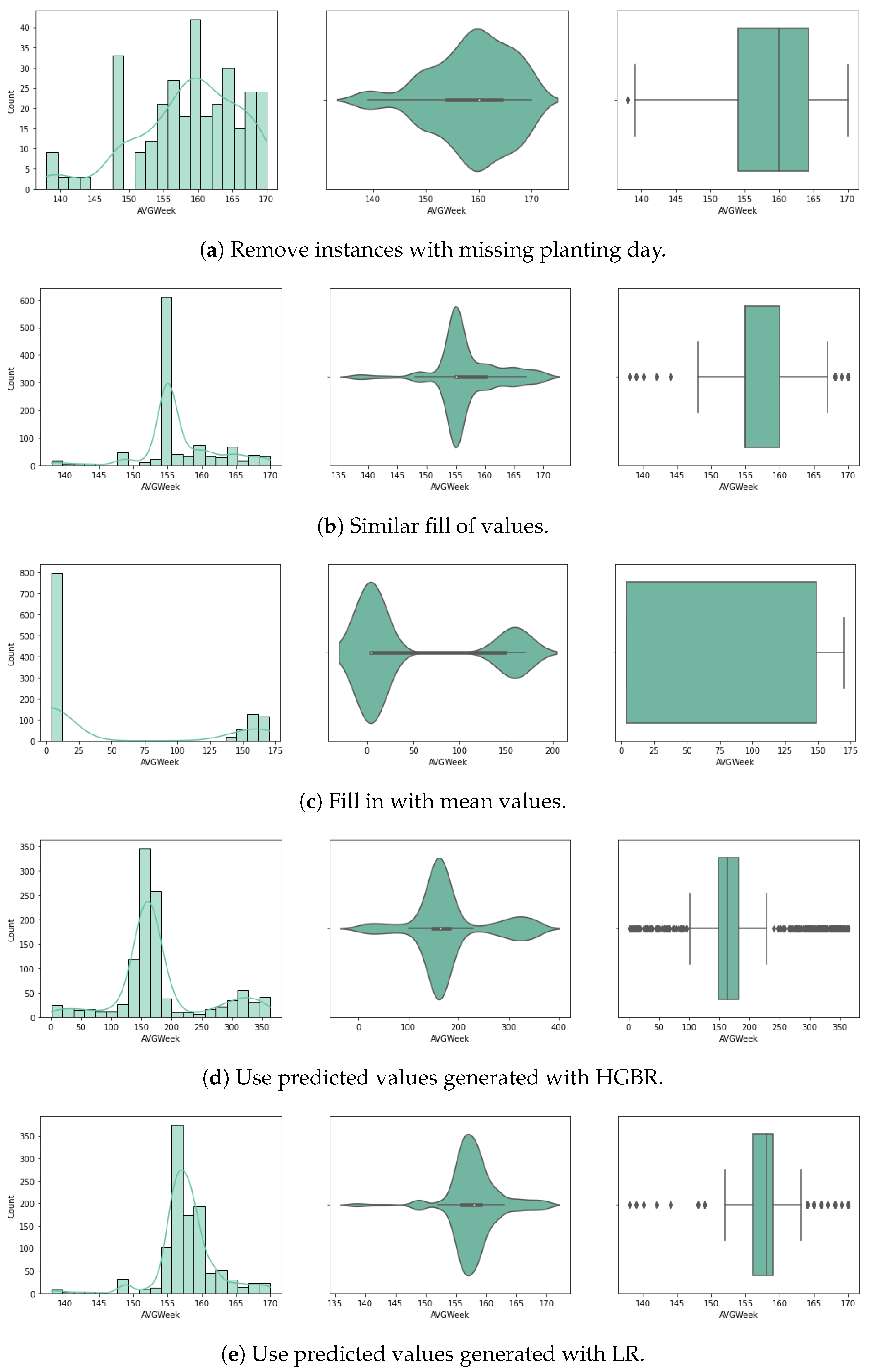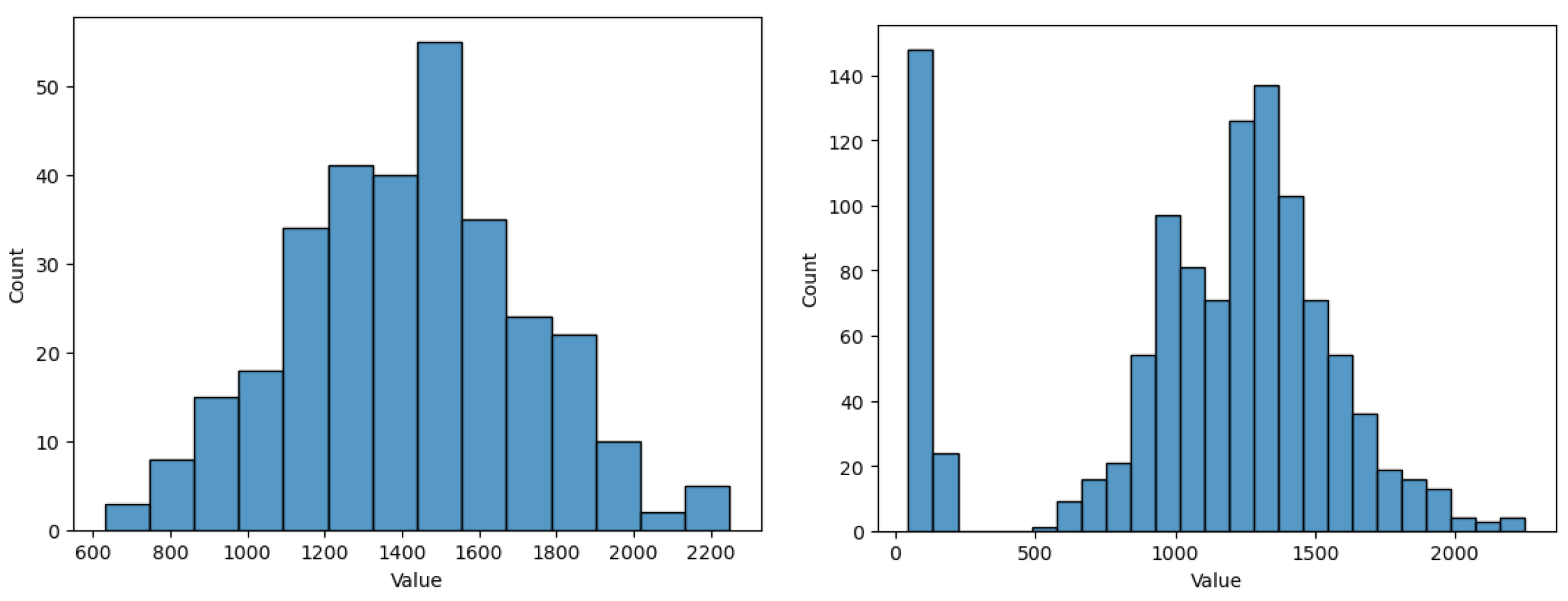In Figure 3 and Figure 4 we visualise the value distribution graph for the planting day feature after using each method.

The first method involves the removal of incomplete instances from the dataset. While this is one of the most common approaches with incomplete data, it results in our case with the loss of 80% of our dataset, with very few remaining instances to train the models. Since the sowing day is central to our experiments in predicting the crop yield, we also considered other approaches.

The second approach is to fill the null values with adjacent ones. For this method, the forward fill ($ffill$) Pandas DataFrame algorithm was used. Given that the data was sorted by state, the missing values were completed with similar values of planting day for the same state, by duplicating the last existing value for that state. This method is also called hot-deck imputation. Although the values would closely correspond to real planting days for that state, given its specific climate context, the risk is that we might introduce inconsistencies corresponding with the meteorological data and yearly variations occurring that interfere with the planting day.

The third approach is to complete with mean values. For this method, we complete all missing values with the overall mean value of the planting day from the dataset. This method is commonly applied as it has the advantage of not introducing statistical changes. However, a great disadvantage is that it cannot simulate seasonality or trends.

For the fourth approach we use prediction to fill in the missing data. Several algorithms have been used to generate univariate prediction models for missing values, informed by the literature review, to perform effectively on similar data and missing data rates [13], including (1) linear regression (LR), (2) histogram gradient boosting regressor (HGBR), (3) extreme gradient boosting tree regressor (XGBT), and (4) random forest (RF). In our case, this approach is expected to be better than using the mean values, provided that the models can predict based on all other features, with more accuracy, based on a trend expected to influence the data.

For this purpose, we have split the dataset in two: dataset A containing the instances missing the value for the planting day, and dataset B containing the complete rows. Next, we created a prediction model using dataset B for training, based on the attributes year, state ANSI, crop type and yield, with target planting day. In the next step, this model was used on dataset A to predict all the missing values for the planting day. Finally, the two datasets were joined again to be used further, together with meteorological data, to predict the yield.

The fifth method consists in the use of an interpolation method. In this approach, the null values of the planting day have been filled using interpolation. This is a statistical method for estimating unknown values based on several known points. The estimation refers to points in between the known values. Here, we used linear interpolation, which estimates a linear polynomial for curve fitting. The pad method was also used, which fills the dataset in with existing values (similar to a hot-deck imputation method). A third interpolation method is spline, which involves fitting the data to several low-degree polynomials. The implementations used in this study are part of the Python Sklearn interpolate() method, with each of the three options.

3.2.2. Handling Outliers

The purpose of outlier detection (OD) is to identify and separate outliers in a sample (anomalies from usual data) from normal data (also called inliers). This is usually an unsupervised problem, as there is not enough knowledge about the data patterns. The general scope of OD algorithms is to allow for the identification of outliers, as their removal from the dataset can be crucial to improving model performance [26].

The crop data involved in the study contained self-reported information filled in by the farmers in a national statistics information platform. A first analysis of the data showed a small percentage (5–10%) of inconsistent or incomplete data (for example, the percentage of planting per week was not filled in for all weeks). This is normal for data collected in an uncontrolled manner. Furthermore, the missing data on planting day were completed using various methods, generating values for 80% of the instances. This is likely to have either introduced or exacerbated anomalies in the dataset.

Given these reasons, we analysed the impact of removing outliers from our data to create the prediction models. In this sense, we applied and compared the unsupervised algorithms for anomaly detection described below, chosen based on the robustness and computation requirements for the regression tasks, as found in the literature.

Isolation forest (IF) uses isolation trees to separate each instance from the rest, and compute the anomaly score from the expected path length $E\left(h\right(x\left)\right)$ of each instance, with $h\left(x\right)$ as the average estimation path length and $c\left(n\right)$ defined based on $H\left(i\right)$, the harmonic number.

$$c\left(n\right)=2H(n-1)-2(n-1)/n$$

(2)

$$s(x,n)=2^{-E\left(h\right(x\left)\right)/c\left(n\right)}$$

(3)

This method is very flexible, as it has been proven to work well even in high-dimensional problems (even for a large number of irrelevant attributes), or in the case where the training set does not contain anomalies [29]. It can be configured by the number of trees and contamination rate (expected rate of outliers in the dataset).

Minimum covariance determinant (MCD) uses a statistical covariance distance to compute a tolerance ellipse, defined as the set of p-dimensional points x whose Mahalanobis distance

$$MD\left(x\right)=d(x,\overline{x},Cov\left(X\right))=\sqrt{{(x-\overline{x})}^{\prime }Cov{\left(X\right)}^{-1}(x-\overline{x})}$$

(4)

describes the distance from the centre of the data cloud to x [30]. The elliptic envelope (EE) implementation in Sklearn was used in our case, as described by [31], and requires setting the contamination rate parameter.

The Local outlier factor (LOF) approach defines LOF of an instance p as

$$LO{F}_{MinPts}\left(p\right)=\frac{{\sum }_{o\in N_{MinPts}\left(p\right)}\frac{lr{d}_{MinPts}\left(o\right)}{lr{d}_{MinPts}\left(p\right)}}{N_{MinPts}\left(p\right)}$$

(5)

the degree to which we call p an outlier, calculated as the average of the ratio of the local reachability density of p (that is, the average reachability distance based on the MinPts-nearest neighbours of p) and those of p’s MinPts-nearest neighbours. The reachability distance of object p with respect to object o is calculated as the distance between an object and the k-neighbourhood of p:

$$reachdis{t}_k(p,o)=max\{kdistance\left(o\right),d(p,o)\}$$

(6)

OneClass-SVM (OC-SVM) is a kernel-based algorithm focused on estimating the density function of the input data (K) in order to define a binary function that decides if a point is an outlier or inlier based on an anomaly detection sensitivity [32]. In short, this involves solving a dual optimisation problem, defined formally as:

$$\underset{\alpha \in R^n}{min}\{\frac{1}{2}{\alpha }^{\gamma }K\alpha \}s.t.\{{\alpha }^{\gamma }1=1,0\le \alpha \le \frac{1}{\nu N}\}$$

(7)

where K is a Gaussian kernel function, $\gamma$ is the kernel scale, and $\nu \in (0,1]$ measures the anomaly detection sensitivity [26]. The $\nu$ hyperparameter needs to be optimised, considering a low value involves a small chance for a point to be an anomaly.

Figure 5 and Figure 6 show the model variation for each outlier removal method with contamination rates from $c=0.05$ to $c=0.5$, when using the prediction with RF as the imputation method, and the XBGT model, HGBR, for evaluation. The metric used for evaluation is $R^2$. The number of instances remaining in the dataset for each contamination rate applied, further used in model training, is presented in

Table 2. Number of instances remaining in the dataset corresponding to each contamination rate applied.

Contamination	0.05	0.1	0.2	0.3	0.4	0.5
n	934	885	787	689	590	492

. The research problem in this case is to identify the smallest contamination rate to avoid model overfitting while obtaining the best model performance.

Looking at Figure 5 for the XGBT model, we notice that IF increases the performance constantly as the contamination rate increases, suggesting an overfitting trend, and a specialisation of the algorithms to select outliers to specialise the model. EE produces a similar variation, with the exception of a local maximum for $c=0.1$, suggesting that this is a good choice of the anomaly rate. On the other hand, LOF presents a local maximum for $c=0.2$, and then performance decreases for higher contamination rates, meaning higher contamination rates will lead to a loss of relevant information for the model. OC-SVM is similar with LOF, with the exception that the local maximum is at $c=0.3$. Figure 6 presents very similar patterns for the HGBR model to those expressed in Figure 5.

For each of the algorithms presented above, we used the Python Sklearn implementations: IF, LOF, EE (for MCD) and OC-SVM. Considering the experiments with different contamination rates and their impact on the model, the proposed candidates for the best results were 0.1, 0.2 and 0.3. Considering the literature recommendations for the contamination rate to avoid model overfitting and the limited data available in our case, we decided on the value $c=0.1$ for our future experiments. For larger datasets of this type, a better choice could be $c=0.2$, provided it was collected similarly in an uncontrolled environment without specific validation.

3.3. Training and Testing

After data preprocessing, involving each of the 10 different approaches for handling missing values for the planting day, the crop data were aggregated with the meteorological data, resulting in 41 features. The dataset was used to train several regression models using a selection of algorithms suitable for this purpose, as exhibited by the state-of-the-art methods and our previous experiments on similar data [33]. The target was chosen to be the yield value field, while all the other 40 features were used as the input.

3.3.1. Histogram Gradient Boosting Regressor

The HGBR is based on ensemble decision trees. The algorithm adds new corrective models in a greedy stepwise manner to improve performance by reducing the square error loss function until it is acceptable [34]. The histogram is an efficient data structure used by the tree-building algorithm to accelerate the process.

3.3.2. Extreme Gradient Boosting Regressor

The XGBT is also a tree-based algorithm. By using a scalable end-to-end gradient boosting tree system, it optimises resource use, introducing cache access patterns, data compression, and block sharding [35].

3.3.3. Hyperparameter Fine-Tuning

The hyperparameters were fine-tuned by experimenting with ranges of significant values, while also balancing the computation time. The best results for the XBGT were obtained using 700 estimators, a maximum depth of 10 and a learning rate of 0.01. For the HGBR we selected a learning rate of 0.002, the maximum number of iterations to be 5000 and the Poisson loss function.

3.4. Validation Metrics

Several metrics have been used to validate and compare the models, based on literature recommendations: the coefficient of determination $R^2$ (considered among the most reliable metrics for regression), the $MAE$, and the $MAE\%$ defined below [36].

The coefficient of determination $R^2$ measures the variation in the y observed values, where $\overline{y}$ is the mean, and is calculated using the equation below [37,38]:

$$R^2=1-\frac{{\sum }_{i=1}^n{(y_i-{\widehat{y}}_i)}^2}{{\sum }_{i=1}^n{(y_i-\overline{y})}^2}$$

(8)

The $MAE$ represents an average of the absolute prediction error with $y_i$ as the observed value and ${\widehat{y}}_i$ as the predicted value, as computed in Equation [38]:

$$MAE=\frac{1}{n}\sum _{i=1}^{n}abs(y_i-{\widehat{y}}_i)$$

(9)

Another metric used is the $MAE\%$ or median absolute percentage error ($MdAPE$) [36], which measures $MAE$ as a percentile from the mean of the y values, as in Equation:

$$MAE\%=\frac{MAE}{\frac{1}{n}{\sum }_{i=1}^n{y}_i}\times 100$$

(10)

We used repeated k-fold cross validation with $k=10$, computing the mean and standard deviation for five repeats, for each of the metrics $R^2$ and $MAE$.

4. Results

Table 3. Comparative results of using different preprocessing imputation methods for handling missing values, including all data in training (without removing outliers).

	XGBT		HGBR
Method	${\mathit{R}}^2$	$\mathit{MAE}$	${\mathit{R}}^2$	$\mathit{MAE}$
Remove missing	0.723 (0.127)	111.645 (20.084)	0.740 (0.142)	107.288 (21.944)
Similar fill	0.918 (0.024)	90.300 (10.402)	0.922 (0.023)	87.315 (10.608)
Mean values	0.915 (0.027)	91.202 (9.206)	0.919 (0.027)	87.669 (9.091)
Predict (LR)	0.920 (0.025)	88.667 (10.325)	0.922 (0.025)	86.593 (10.464)
Predict (HGBR)	0.925 (0.024)	85.395 (9.903)	0.927 (0.023)	84.427 (10.156)
Predict (XGBT)	0.926 (0.022)	84.052 (8.762)	0.928 (0.022)	83.031 (9.039)
Predict (RF)	0.929 (0.023)	82.050 (9.385)	0.929 (0.022)	81.483 (9.387)
Interpolation (L)	0.918 (0.024)	90.685 (10.332)	0.922 (0.022)	87.687 (10.339)
Interpolation (P)	0.918 (0.024)	90.300 (10.402)	0.922 (0.023)	87.315 (10.608)
Interpolation (S)	0.918 (0.024)	90.685 (10.332)	0.922 (0.022)	87.687 (10.339)

The numbers in the table represent the mean values, with the standard deviation (SD) value in parenthesis, calculated from five repetitions of the 10-fold cross validation. For example, the $R^2$ when we remove the instances containing missing values is 0.687 (0.119), that is: the mean value is 0.687 with $SD=0.119$. Method notations: LR—linear regression; RF—random forest; L—linear; P—pad; S—spline.

shows the comparison between several metrics obtained by the selected algorithms, when using each of the five approaches (presented in the Section 3) in dealing with missing data regarding the planting date. In our case, we are dealing with 984 instances with 41 attributes, of which 80% of the instances are only missing the planting date attribute, and was completed using imputation methods. In this table, we also included the evaluation of the model for the case when the instances with missing data were removed ($n=312$). The mean yield value is 1093.053, meaning the $MAE$ of 87.628 represents a percentile error of $MAE\%=$8.01%, and all $MAE$ values under 100 have a corresponding $MAE\%$ under 10%.

We notice that the $R^2$ values increase when imputation is used as opposed to removing incomplete data instances: from 0.723 for XBGT and 0.740 for HGBR to values in the range of 0.918–0.929 for the different imputation utilised methods. Accordingly, the $MAE$ was reduced from 111.645 for XGBT (remove missing) to 81.483–91.202, meaning a reduction in $MAE\%$ from 10.2% to 7.44% in the best case. Therefore, the first important result is that the imputation step greatly improves our model, regardless of the approach used. However, it can still be further fine-tuned and improved.

The next step was to handle outliers in our data.

Table 4. Comparative results of using different preprocessing methods for missing values, after removing outliers with Isolation Forest.

	XGBT		HGBR
Method	${\mathit{R}}^2$	$\mathit{MAE}$	${\mathit{R}}^2$	$\mathit{MAE}$
Remove missing	0.743 (0.167)	106.242 (19.641)	0.752 (0.163)	102.309 (17.622)
Similar fill	0.928 (0.019)	88.156 (10.262)	0.927 (0.024)	86.301 (10.678)
Mean values	0.928 (0.022)	85.868 (10.136)	0.930 (0.022)	83.769 (10.009)
Predict (LR)	0.930 (0.020)	85.632 (10.274)	0.930 (0.021)	85.126 (9.833)
Predict (HGBR)	0.933 (0.021)	82.086 (7.851)	0.934 (0.020)	81.156 (7.867)
Predict (XGBT)	0.937 (0.017)	81.038 (9.599	0.936 (0.018)	81.195 (9.896)
Predict (RF)	0.937 (0.018)	80.106 (9.159)	0.934 (0.019)	81.414 (8.320)
Interpolation (L)	0.927 (0.022)	88.607 (10.667)	0.930 (0.021)	86.025 (9.692)
Interpolation (P)	0.928 (0.020)	86.998 (9.626)	0.929 (0.020)	85.743 (9.561)
Interpolation (S)	0.932 (0.042)	80.357 (13.635)	0.932 (0.041)	80.123 (13.238)

,

Table 5. Comparative results of using different preprocessing methods for missing values, after removing outliers with local outlier factor.

	XGBT		HGBR
Method	${\mathit{R}}^2$	$\mathit{MAE}$	${\mathit{R}}^2$	$\mathit{MAE}$
Remove missing	0.727 (0.130)	108.730 (17.376)	0.753 (0.118)	103.766 (16.987)
Similar fill	0.925 (0.019)	88.245 (9.865)	0.928 (0.017)	85.205 (9.155)
Mean values	0.927 (0.022)	87.068 (10.362)	0.929 (0.022)	84.388 (10.372)
Predict (LR)	0.926 (0.022)	86.516 (10.893)	0.928 (0.023)	84.766 (11.757)
Predict (HGBR)	0.930 (0.024)	84.503 (10.754)	0.931 (0.023)	84.027 (10.103)
Predict (XGBT)	0.931 (0.032)	81.576 (10.299)	0.934 (0.030)	79.629 (10.327)
Predict (RF)	0.934 (0.022)	78.954 (10.882)	0.936 (0.021)	78.223 (11.116)
Interpolation (L)	0.921 (0.018)	91.107 (9.300)	0.925 (0.018	87.509 (8.895)
Interpolation (P)	0.925 (0.019)	88.245 (9.865)	0.928 (0.017)	85.205 (9.155)
Interpolation (S)	0.921 (0.018)	91.107 (9.300)	0.925 (0.018)	87.509 (8.895)

,

Table 6. Comparative results of using different preprocessing methods for missing values, after removing outliers with MCD.

	XGBT		HGBR
Method	${\mathit{R}}^2$	$\mathit{MAE}$	${\mathit{R}}^2$	$\mathit{MAE}$
Remove missing	0.739 (0.111)	109.408 (20.823)	0.749 (0.103)	106.983 (20.386)
Similar fill	0.924 (0.023)	89.103 (9.608)	0.926 (0.021)	86.565 (9.551)
Mean values	0.925 (0.020)	90.240 (9.794)	0.929 (0.018)	86.750 (9.041)
Predict (LR)	0.927 (0.023)	87.129 (11.312)	0.927 (0.024)	85.118 (11.361)
Predict (HGBR)	0.929 (0.025)	85.901 (11.576)	0.930 (0.025)	84.633 (11.123)
Predict (XGBT)	0.930 (0.024)	83.389 (11.251)	0.931 (0.023)	83.619 (11.172)
Predict (RF)	0.935 (0.027)	78.590 (11.139)	0.935 (0.027)	78.853 (11.647)
Interpolation (L)	0.927 (0.016)	89.823 (8.578)	0.930 (0.016)	85.956 (8.972)
Interpolation (P)	0.922 (0.026)	90.298 (10.035)	0.925 (0.025)	87.253 (10.146)
Interpolation (S)	0.924 (0.021)	90.676 (10.070)	0.929 (0.020)	86.279 (10.069)

and

Table 7. Comparative results of using different preprocessing methods for missing values, after removing outliers with OC-SVM.

	XGBT		HGBR
Method	${\mathit{R}}^2$	$\mathit{MAE}$	${\mathit{R}}^2$	$\mathit{MAE}$
Remove missing	0.750 (0.100)	105.738 (19.072)	0.766 (0.103)	101.952 (20.124)
Similar fill	0.928 (0.019)	86.783 (9.188)	0.931 (0.018)	83.636 (9.205)
Mean values	0.929 (0.020)	86.062 (9.985)	0.932 (0.019)	83.714 (9.608)
Predict (LR)	0.928 (0.019)	86.347 (9.696)	0.929 (0.019)	84.630 (9.602)
Predict (HGBR)	0.934 (0.022)	82.611 (10.374)	0.934 (0.021)	82.107 (9.662)
Predict (XGBT)	0.935 (0.020)	81.085 (10.845)	0.936 (0.019)	80.581 (9.695)
Predict (RF)	0.937 (0.017)	77.262 (8.176)	0.938 (0.017)	77.689 (7.980)
Interpolation (L)	0.925 (0.021)	88.573 (8.675)	0.927 (0.020)	85.441 (8.142)
Interpolation (P)	0.928 (0.019)	86.783 (9.188)	0.931 (0.018)	83.636 (9.205)
Interpolation (S)	0.925 (0.021)	88.573 (8.675)	0.927 (0.020)	85.441 (8.142)

show the results obtained after using each of the four outlier removal methods. The notations used in these tables are as explained in Table 3.

We notice that the results presented in these tables show that there is improvement for all the imputation methods and the outlier removal technique applied, with the best value for HBGR when using RF for the imputation and OC-SVM for the removal of outliers: $R^2=0.938$, $MAE=77.689$, and $MAE\%$ = £7.06%. To assess the relevance of the improvement, we applied the statistical t-test between the models based on all data and each outlier model. The obtained p values for these metrics show they are statistically significant in most cases, with values of $p<0.05$ in half the cases (as detailed in

Table 8. p values for each outlier removal method versus none.

		IF	LOF	MCD	OC-SVM
XGBT	$R^2$	$p=3.78$	$p<0.01$	$p=2.55$	$p=1.36$
	$MAE$	$p<0.01$	$p<0.01$	$p<0.05$	$p=2.19$
HGBR	$R^2$	$p=2.96$	$p=5.23$	$p<0.01$	$p=9.88$
	$MAE$	$p<0.01$	$p<0.01$	$p<0.03$	$p=5.14$

).

Figure 7 and Figure 8 present all these results for the combination of outlier method or no outlier method removal used (meaning all data is involved in constructing the model) and the two evaluation algorithms used thus far (XGBT and HGBR), for the metrics $R^2$ and $MAE$, respectively, in the form of box plots. From these we can see that based on the median value (in orange) and overall performance (minimum and maximum values, as well as the interquartile range—IQR), IF is the outlier removal method with the highest improvement on the models overall, followed by OC-SVM, for both the $R^2$ and $MAE$ metrics. The circles in the graph represent outlier values (at a distance greater than $Q1-1.5\times IQR$ or $Q3+1.5\times IQR$), providing the best $MAE$ results for LOF and OC-SVM, with the overall best performance being OC-SVM for both $R^2$ and $MAE$, while these prove to be the best approaches numerically, we are inclined to interpret them as outliers resulting form the statistical 10-fold cross-validation data split performance of five repetitions.

5. Discussion

In terms of answering the research question regarding using imputation or not when 80% of the information for one feature is missing (considering that we have a total of 41 features as presented in Figure A1 from Appendix A), the preference would be towards the first option. Regardless of the method used for imputation, the model proved to be more accurate in all cases. On the other hand, given that we would lose 80% of the data, the risk is also to use other particularities in building the model.

To emphasise this, in Figure 9 we analysed the yield value histogram when removing instances with missing planting day, compared to using all initial instances (which contain a second peak for the histogram distribution, suggesting perhaps a separate class cluster among the initial data, which seems to be representative, and not just outliers). From this figure we notice the need for imputation to preserve relevant data, otherwise some characteristics of the model are lost. When missing data instances are removed, the values between 0 and 500 for the yield are no longer present. However, they represent relevant data for some types of crops, even if they do not represent the majority of crop types, thus losing a component. Of course, one can argue here that an extra component could be approached by building separate models. For our case, we continue to consider them as a whole, part of the same model.

To better visualise this, we rendered in Figure 10 a plot of the actual vs. predicted values, for the best result obtained, involving HGBR as the regression model, OC-SVM the unsupervised outlier removal method, and RF as the prediction imputation method. On the left, we have the plot obtained for the prediction model based on the data from which we removed instances with missing values. On the right, we have the model built using imputation, where we notice a linear trend involving two main clusters, one between 0 and 500 and one between 500 and 2500 for the yield value, in line with the histogram for the yield for the initial data. On the other hand, the left plot shows only one group, with the 0–500 yield value range missing. This shows that by removing data, we lose relevant information for the model, and the preprocessing methods involved, using imputation and outlier removal, are able to create a much more robust and reliable prediction model.

For the research question on which imputation method produces the best model, prediction is preferred to all others in all cases, with RF algorithms producing the highest values for $R^2$. The same trends in model improvement are present for both XGBT and HGBR, proving that the change in performance is mainly due to the preprocessing methods used, for both imputation and outliers removal.

For the latter, concerning data anomalies and unsupervised outlier removal, further experiments would be required to establish if it can be more accurately fine-tuned and if higher contamination rates, such as $c=0.2$, could be feasible to use in a larger dataset or if it would lead to model overfitting. Looking back at the results in Figure 5 and Figure 6, showing the variation of the model prediction for the coefficient of determination metric, the best results are obtained by OC-SVM when $c=0.3$ ($R^2=0.95$ for both XBGT and HGBR), and LOF when $c=0.2$ ($R^2=0.943$ for XBGT and $R^2=0.945$ for HGBR). For EE there is a local peak at $c=0.1$, and a maximum value at $c=0.5$, while IF improves as c is increased (with a maximum at $c=0.5$). More information on the initial data and the collection context could help inform the actual anomaly percentage present in the data, and what approach would indeed improve the model.

Another aspect to discuss is in relation to the regression algorithms XGBT and HGBR, which seem to be quite robust, showing little impact from unsupervised outlier removal, as opposed to the other regression algorithms which are more susceptible to data changes. However, a main finding of our study is that it is feasible and we can reliably use these algorithms for crop yield prediction even with relatively small datasets. However, we must provide a minimum amount of data to ensure performance, thus demonstrating the importance of using imputation. The most important contribution we bring is related to the problem of missing data, which can be handled effectively even if it affects 80% of the instances, resulting in an increased performance from 0.723 to 0.938 (and even up to 0.95 if we use OD with $c=0.3$). Our findings suggest that the best method for imputation is prediction using RF. Given that historical crop data are reduced and it would take many years to collect a designated dataset (which we have started as a work in progress), we are able to address the climate change effects in agriculture now, by modelling the correlation between sowing dates and weather forecast to identify the best planting window that maximises yield production.

6. Conclusions

The presented paper completes the research in the field of intelligent agro-meteorological decisions to address the challenges of ensuring the sustainable provision of food crops in the context of climate change. Although there are multiple studies in the field, a new, unique approach that addresses missing data is needed.

The primary objective of our research was to improve the efficiency of sunflower cultivation by developing a yield prediction model that relies on the selection of an optimal planting day, guided by a region-specific weather forecast. In order to construct a regression model capable of accurately predicting crop yield, we aggregated several datasets encompassing information pertaining to crops, planting dates, crop varieties, geographical locations, and historical yield records. Additionally, meteorological parameters such as precipitation and temperature were incorporated into the model as predictors.

Moreover, in our experiments, we performed a comparative study of nine imputation methods, which were evaluated on two regression algorithms. We obtained an increase in the model performance for both regression algorithms. The best results were obtained using the prediction method for imputation, especially the RF. The second set of experiments involved unsupervised outlier removal algorithms, in which four methods were compared with various contamination rates. Overall, results were improved in most cases with statistical significance. The best $R^2=0.938$ and $MAE=77.689$ were obtained using the Oc-SVM outlier removal and RF imputation algorithms, for the model built with HGBR. An important finding is that a very significant improvement was mainly achieved through preprocessing methods, compared to the initial results without imputation or outlier removal ($R^2=0.723$).

We have been able to achieve our research objective and build an accurate model based on limited data, which could support agricultural decisions to mitigate the effects of climate change and maximise production. Future research directions involve incorporating more variables as predictors, such as the use of fertilisers or pest control. There is a substantial need to collect crop datasets specific to this purpose from reliable sources to help train models for specific geographical locations and crops. As a further exploration of the impact of the planting day and weather conditions on the crop yield, we aim to also consider employing forecasting methodologies and assessing the reliability of using the same or similar preprocessing methods to improve the model performance.