Machine Learning Algorithms for Raw and Unbalanced Intrusion Detection Data in a Multi-Class Classification Problem

Abstract

Various machine learning algorithms have been applied to network intrusion classification problems, including both binary and multi-class classifications. Despite the existence of numerous studies involving unbalanced network intrusion datasets, such as CIC-IDS2017, a prevalent approach is to address the issue by either merging the classes to optimize their numbers or retaining only the most dominant ones. However, there is no consistent trend showing that accuracy always decreases as the number of classes increases. Furthermore, it is essential for cybersecurity practitioners to recognize the specific type of attack and comprehend the causal factors that contribute to the resulting outcomes. This study focuses on tackling the challenges associated with evaluating the performance of multi-class classification for network intrusions using highly imbalanced raw data that encompasses the CIC-IDS2017 and CSE-CIC-IDS2018 datasets. The research concentrates on investigating diverse machine learning (ML) models, including Logistic Regression, Random Forest, Decision Trees, CNNs, and Artificial Neural Networks. Additionally, it explores the utilization of explainable AI (XAI) methods to interpret the obtained results. The results obtained indicated that decision trees using the CART algorithm performed best on the 28-class classification task, with an average macro F1-score of 0.96878.

1. Introduction

Intrusion Detection Systems (IDS) play a key role in strengthening organizational security by providing an additional layer of defense to detect and respond in time to potential threats that may have bypassed preventive measures. These systems can detect a wide range of threats, including malware, phishing attacks, and other types of cyber-attacks, that may be missed by more traditional security solutions [1]. As digital networks become more complex and interconnected, the potential for vulnerabilities and weaknesses in the system increases, making it more difficult to identify and prevent all potential threats. IDSs can help to address this problem by providing continuous monitoring and analysis of network traffic, helping to identify potential threats before they can cause significant damage, but the development of a reliable and effective system may still be a challenging task.

IDSs must be designed to identify and respond to a wide range of cyber threats, including new and emerging attack techniques and to process massive amounts of network traffic data in real time, which can be challenging in terms of both computational resources and data processing speed [2]. This requires careful optimization of IDS algorithms and systems to ensure that they can process large volumes of data in a timely and efficient manner.

IDSs typically rely on a variety of techniques, such as signature-based detection [3,4], anomaly detection [5,6] and machine learning algorithms [7,8], to identify potential threats. Nevertheless, addressing class imbalance is a frequent challenge in machine learning and data analysis, especially when working with datasets in which the occurrence of one class is significantly less frequent compared to the others. In the context of network traffic analysis, this can be a problem because most of the traffic is typically benign, while malicious traffic is relatively rare. Many papers propose to deal with this problem by leaving only two types of attack—benign and malignant [9,10,11]—to reduce the number of classes in the grouping [12], but knowing which type of attack is also important.

Class imbalances can pose a number of challenges for researchers and data analysts, such as reducing the effectiveness of certain classification models and causing interpretation and generalization problems that may lead to biased or inaccurate results [13]. However, there are other factors that can also contribute to this issue. One of these factors is the overlap of classes due to a lack of feature separation, which can make it difficult for the algorithm to distinguish between the different classes. In addition, a lack of attributes that are specific to a certain decision boundary can make it difficult for the algorithm to accurately classify data. In recent years, deep learning techniques, including convolutional neural networks (CNNs) [14,15], recurrent neural networks (RNNs)) [16,17], and deep belief networks (DBNs)) [18], have gained significant attention for their promising capabilities in various classification tasks. Particularly in the field of cybersecurity attack classification, deep learning approaches have been increasingly utilized to exploit their potential.

While accuracy is very important, there is a growing demand for algorithmic transparency and the “white box” principle, particularly in the field of intrusion detection. This demand is driven by the need to understand and explain the decisions made by an IDS and to ensure that these decisions are fair, unbiased and explainable [19,20].

In recent years, the emergence of the XAI (explainable Artificial Intelligence) paradigm has played an important role in making algorithms more transparent and understandable [21]. XAI aims to create transparent, interpretable and explainable artificial intelligence models to make it easier to understand how these models make decisions. In the context of intrusion detection, XAI can help identify the features that are most influential in the decision-making process and why a certain output is obtained [22,23,24]. Similarly, in intrusion detection, an XAI system can explain to the intelligent system user why a particular network activity has been flagged as suspicious or anomalous and provide insights into the underlying patterns or trends that led to the detection. By providing interpretable insights, XAI can help security analysts to understand how the system is identifying and classifying network traffic and to make more informed decisions on how to respond to potential threats [25,26].

This study addresses the challenges of understanding network intrusion multi-class classification results on a highly imbalanced dataset (CIC-IDS2017 and CSECIC-IDS2018) using different machine learning (ML) models, such as Logistic Regression, Random Forest, Decision trees, Multilayer Perceptron and dense-layer network. The paper conducted a comparative analysis of the classification results of machine learning models using various accuracy metrics. Moreover, specific explainable AI (XAI) methods, including local and global explanation models, have been employed to evaluate the capabilities and robustness of XAI in identifying the crucial features within the dataset that significantly influence the classification results.

2. Related Works

The CIC-IDS2017 dataset is a well-known benchmark dataset for Intrusion Detection Systems (IDS). It contains network traffic data collected from real-world environments with different types of attacks and normal traffic. The initial dataset consisted of 79 features and 15 classes (one benign, 14 malicious). To enhance the classification performance of this dataset, numerous studies have been conducted, incorporating detailed analyses such as feature selection, class grouping, data cleaning, and processing. For this task, a wide range of classifiers have been employed, including classical methods, such as Random Forest RF [27,28] and MLP (multi-layer perceptron) [13,28] as well as deep learning architectures [29,30,31,32,33].

Table 1. Multi-classification accuracy results for the CIC-IDS2017 dataset.

Method	Classifier	F1-Score, (%)	Classes
Zachariah Pelletier [27]	ANN	96.53	13
	RF	96.24
Amer A.A. Alsameraee et al. [28]	RF	98.36	6
	MLP	80.63
	Naive Bayes (NB)	90.82
Mariama Mbow et al. [29]	LSTM	98.65	15
	4 layers CNN	98.98
Hongpo Zhang [30]	SGM-CNN	96.36	15
Razan Abdulhammed et al. [31]	PCA+RF	99.60	15
Petros Toupas et al. [32]	8 hidden layers DenseNet	94.10	13
Yong Zhang [33]	Parallel cross convolutional neural network (PCCN)	99.68	12

presents the results of specific multi-class classification studies, displaying the F1-score and the corresponding number of classification classes. The majority of the results demonstrated an accuracy exceeding 90%, regardless of whether the classification involved 15 or fewer classes.

Due to class imbalance, which is prevalent in the CIC-IDS2017 dataset and numerous other cybersecurity datasets, one class, specifically Benign, dominates the others, accounting for 80.3% of the raw data. To tackle this issue, various approaches have been employed, resulting in variations in the number of classes across different studies. Methods such as resampling [12], ensemble learning [34] or employing simple binary classification [9,34] have been frequently utilized in addressing class imbalance. One of the main issues encountered in the CIC-IDS2017 dataset is the incorrect aggregation of packets into streams, primarily caused by inadequate protocol detection. This problem has an impact on the number of classes or attributes within the dataset [35,36]. As a result, flows in the dataset may be too short or too long or may consist of packets from different conversations, resulting in inaccurate flow attributes. In addition, there are problems with TCP session termination in the dataset, so similar flows may have different labels. The presence of inaccurate flow attributes resulting from incorrect packet aggregation can introduce complexities that may confuse machine learning algorithms, consequently rendering the detection of network intrusions more challenging.

The CSE-CIC-IDS-2018 dataset contains a total of 28 classes of network traffic, each representing a different type of network activity. However, in classification tasks, these classes are often aggregated into 7 groups, namely “Benign”, “DDoS”, “DoS”, “Brute Force”, “Bot”, “Infiltration”, and “Web.” Occasionally, the classes are collapsed into 10 groups, and the maximum number of classes observed for classification is 14, as depicted in

Table 2. Multi-classification accuracy results for the CSECIC-IDS2018 dataset.

Method	Classifier	F1-Score, (%)	Classes
Jumabek, Alikhanov et al. [37]	DT(CART)	87.36	13
	RF	88.13
	CatBoost	88.84
L. Liu et al. [38]	DSSTE + miniVGGNet	97.04	14
	DSSTE + AlexNet	96.49
	DSSTE + LSTM	96.50
Jofrey L. Leevy [39]	CatBoost	91.65	7
	LightGBM	94.69
	DT	88.58
	LR	49.47
	NB	24.31
	RF	92.94
	XGBoost	93.64
Farhan, Baraa Ismael et al. [40]	LSTM	99.00	10
Ilhan Firat Kilincer et al. [41]	LGBM (Light GBM)	99.94	7
	XGBoost	99.92
Saud Alzughaibi et al. [42]	MLP-BP (Multi-layer perceptron + backpropagation)	99.20	7
	MLP-PSO (multi-layer perceptron + particle swarm optimization)	97.60

.

It has been observed that hybrid deep learning architectures tend to outperform other machine learning algorithms in terms of accuracy results. All these studies have shown that the majority of F1-scores are above 95% for classifications of up to 14 classes. In addition, such common metrics as recall, precision, ACC (Accuracy) and F1-score are provided, but the weighted average F1-score is a more useful metric in this case, as it takes into account the relative importance of each class in terms of its support, which is particularly important for unbalanced datasets. Macro averaging is another commonly used technique for evaluating performance metrics in highly imbalanced datasets; however, none of these metrics were provided in the studies.

Many studies have reported promising results using deep learning architectures on this dataset, classifying network traffic as either benign or malicious (as a binary classification task) [9,11,43]. However, this does not mean that increasing the number of classes will always result in decreased accuracy, and such trends have not been observed.

Observations have indicated that the impact of model architecture or hyperparameters on accuracy is minimal [9,44]. Instead, factors such as training and testing data, data processing and preparation, the number of sampled features and other similar considerations have a more significant influence. Nevertheless, there remains uncertainty regarding whether more complex hybrid models actually yield more accurate results. Additionally, questions persist regarding the rationale and benefits of merging classes, conducting extensive data cleaning, or reducing features. Thus, in this study, experiments were carried out separately on the raw CIC-IDS2017 and CSE-CIC-IDS-2018 datasets, i.e., keeping the initial number of attack types (the number of classes) at 15 and 28, respectively. For further investigation, these datasets were merged into a single dataset, which resulted in 19,063,686 instances, 79 features (initially 85) and 28 classes.

3. Dataset

The CIC-IDS2017 and CSE-CIC-IDS-2018 (an extension to the CIC-IDS-2017 dataset with more network traffic data) datasets have become popular in the research community, particularly in the field of IDSs. The CIC-IDS2017 dataset was generated from real network recordings.

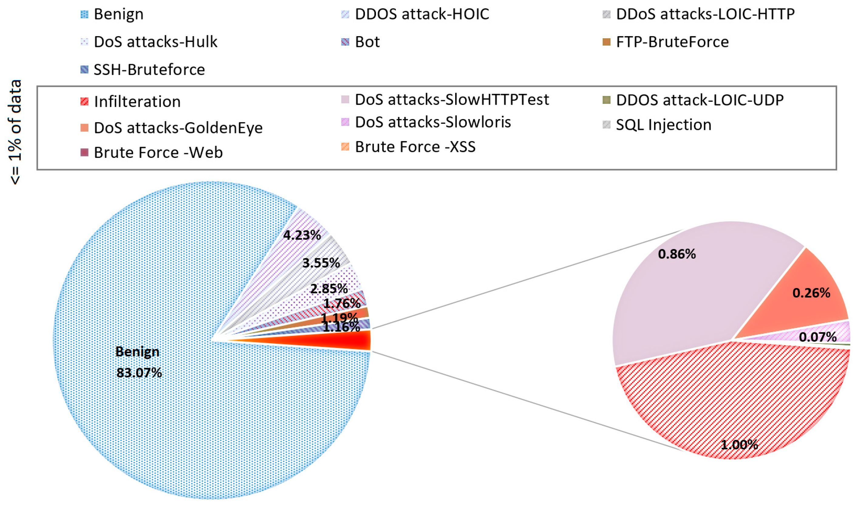
The data collection period started on Monday 3 July 2017 at 9.00 a.m. and ended on Friday 7 July 2017 at 5.00 p.m. for a total of 5 days. Each dataset record contains 79 parameters, the last of which is an output with 15 different names (classes) indicating to which type of malicious activity, if any, the network packet described in the dataset record belongs. All possible output values and their proportions in the overall dataset are shown in Figure 1.

The CSE-CIC-IDS-2018 dataset is larger than the CIC-IDS2017 dataset in terms of the number of flows it contains, with more than 80 million flows compared to about 3 million flows in the CIC-IDS2017 dataset. This dataset includes not only the attack types identified in the CIC-IDS2017 dataset, but also several new attack types commonly found in web applications, such as SQL injection, cross-site scripting (XSS) and command injection. These attacks can be particularly damaging because they target vulnerabilities in the application itself, allowing attackers to gain unauthorized access to sensitive data or to take control of the system. SQL injection attacks and XSS attacks are two common types of web application attacks that can be very harmful. SQL injection attacks occur when an attacker is able to inject malicious SQL code into a web application’s input fields. If the application does not properly validate or sanitize the user input, the malicious code can be executed by the database, allowing the attacker to access, modify or delete sensitive data. XSS attacks, on the other hand, involve injecting malicious scripts into a web application’s pages. This can allow attackers to steal sensitive information, such as cookies or login credentials, or to gain control of the user’s browser, redirecting them to other malicious sites or launching further attacks.

Regarding the output imbalance problem, we can see that the situation is very similar to the 2017 dataset (the dominant class accounts for 82.66% of the dataset), so it would make sense to merge them (see Figure 2). By merging the datasets, the total number of examples in the minority class would increase. Additionally, by keeping only the entries that have a certain number of entries, it would be possible to remove any outliers or rare classes that may not have enough examples to train the classification model effectively.

4. Materials and Methods

4.1. Logistic Regression

Logistic regression is a binary classification algorithm used to predict a binary outcome (i.e., 0 or 1). For multi-class classification tasks, it is better to use an extension of logistic regression, such as Softmax regression, One-vs-Rest (OvR) or One-vs-One (OvO). In this study, we used Softmax regression, also known as multinomial logistic regression. This approach produces a single model that directly models the probability distribution of all K classes. The model learns a set of K linear functions, one for each class, and uses a softmax function to normalize the output to the probability distribution of all K classes. The class with the highest probability was chosen as the output during the prediction. The softmax function for class k is defined as follows:

$$\left(y=k|x\right)=\frac{e^{f_k\left(x\right)}}{{{\displaystyle \sum }}_{j=1}^K{e}^{f_j\left(x\right)}} \mathrm{for} k=1,2,\dots , K$$

(1)

where $f_k\left(x\right)$ is a score of class k for input x. The score can be defined as a linear function.

During training, the parameters of the model (i.e., the weights and biases of the linear functions) are learned using an optimization algorithm that minimizes a loss function. The most commonly used loss function for softmax regression is cross-entropy loss. The cross-entropy loss for a single example $\left(x,y\right)$ is defined as follows:

$$L\left(x,y\right)=-{{\displaystyle \sum }}_{k=1}^K{y}_k·logP(y=k|x)$$

(2)

where $y_k$ is the indicator function, taking the value 1 if the true label is $k$ and 0 otherwise. The class with the highest probability was chosen as the output for the prediction:

$$\widehat{y}=\begin{array}{c}\arg max P(y=k|x)\\ k\end{array}$$

(3)

where $\widehat{y}$ is the predicted class label.

4.2. Decision Trees and Random Forest

Decision trees (DTs) can be used to solve both classification and regression problems and are particularly useful when the data have complex non-linear relationships. DT can be a powerful tool for building intrusion detection technologies, such as firewalls and IDS [45,46,47]. However, DT can be prone to overfitting and can have high variance, which can be addressed by techniques such as pruning or the ensemble method. In this research, we have implemented two DT algorithms—ID3 and CART—and a random forest composed from a set of CART-types trees.

The ID3 (Iterative Dichotomiser 3) algorithm uses Information Gain (IG) to find the best feature to split the data at each node of the decision tree. Information Gain is a measure of the reduction in entropy that can be achieved by splitting the data on a particular feature. The feature with the highest IG was chosen as the split feature at each node, as it is expected to provide the most useful discrimination between the different classes.

$$Entropy\left(S\right)=-{{\displaystyle \sum }}_{i=1}^n{p}_i·lo{g}_2(p_i),$$

(4)

where S represents the dataset that entropy is calculated, i represents the classes in set, and $p_i$ represents the proportion of data points that belong to class i to the number of total data points in set S. The Information Gain formula is provided below:

$$IG\left(S,A\right)=Entropy\left(S\right)-{{\displaystyle \sum }}_{v\in Values\left(A\right)}\frac{\left|S_v\right|}{\left|S\right|}Entropy\left(S_v\right),$$

(5)

where Sᵥ is the set of rows in S for which the feature column A has value v, |Sᵥ| is the number of rows in Sᵥ and likewise |S| is the number of rows in S.

CART (Classification and Regression Trees) is another DT algorithm that can handle both categorical and continuous input variables and is less prone to overfitting than ID3. CART is used for binary splitting, which involves splitting the data into two groups based on the value of a single input variable. To perform binary splitting, the algorithm first evaluates the Gini impurity index:

$$Gini=1-{{\displaystyle \sum }}_{i=1}^C{\left(p_i\right)}^2,$$

(6)

where C is the total number of classes, and $p_i$ probability of selecting a data point with class $i$. The Gini impurity of a pure node (the same class) is equal to zero.

A random forest (RF) is a decision tree-based algorithm that uses an ensemble of decision trees to make predictions [48]. Moreover, it is a very popular technique for network intrusion detection [46,49]. In our case, employing RF, several CART-type decision trees were created using randomly selected subsets of training data and features. Each tree in the forest made a prediction based on the values of the features and provided a class label. The final prediction of the random forest was the dominant class.

$$RF=f\left(D{T}_1,D{T}_2,\dots ,D{T}_n\right)$$

(7)

where $f=mode$, n-number of tress DT in random forest. The $mode$ function returns the most frequently occurring predicted class across all trees.

Theoretically, the RF algorithm has several advantages over a single decision tree in that it can handle high-dimensional, less balanced datasets with many attributes and can reduce overfitting. For this purpose, regularization, bagging and boosting techniques have been applied, as well as pre-pruning methods, which involve setting conditions for the growth of decision trees during the construction of the forest.

4.3. ANN-Type Models

In this study, we implemented two ANN-type models: (1) a multi-layer perceptron (MLP) and (2) a deep learning architecture—the dense-layer network.

Multilayer perceptron (MLP) is a type of ANN composed of neurons that are interconnected and function as individual information processing units, which allows it to learn complex functional relationships between input features and the output [50]. We have implemented MLP with 4 hidden layers, with 64 nodes in the first layer, 128 nodes in the second and third layers, and 64 nodes in the fourth layer. The strength of the L2 regularization term is set to 0.001, which means that the model provides a moderate amount of regularization to the weights of the model. The Rectified Linear Unit (ReLU) function is used as the activation function in the hidden layers. To prevent overfitting, early stopping is enabled and the strength of the L2 regularization term is set to 0.01.

A dense-layer network, also known as a fully connected network, is a type of neural network architecture commonly used in deep learning. In a dense network, each neuron in a given layer is connected to all the neurons in the previous layer, resulting in a dense, fully connected graph of nodes [51]. A neural network with 23 dense layers was used as a deep learning model, incorporating batch normalization, a ReLu activation function and an Add operation with a total of 2,714,780 parameters. The structure of the model architecture is provided in Figure 3.

4.4. Explainable Artificial Intelligence Methods

Machine learning algorithms are increasingly being used in various applications of cybersecurity, such as malware detection, intrusion detection and vulnerability assessment. However, the black-box nature of many machine learning models can make it difficult to understand why they make certain predictions or decisions. XAI technologies are very relevant in the field of cybersecurity, where the consequences of errors or biases in machine learning models can be severe.

Before applying XAI methods, it is important to understand their scope, the stage of system development where XAI can be used and what it can explain [52]. Two different XAI models can be distinguished according to the scope of the explanation: (1) Local; (2) Global models. At the local level, explainability focuses on providing explanations for individual predictions or decisions made by an AI model. Local explainability methods help understand the factors or features that influence a specific outcome. Meanwhile, global explainability aims to explain the overall behavior and decision-making process of an AI model across its entire input space. It focuses on providing insights into the model’s general characteristics, biases and patterns.

Next, it is important to assess at which stage an explanation of the ML model is relevant. Pre-model explainability is the process of explaining an AI model before it is implemented or trained. It focuses on the development and selection of models or algorithms that are intrinsically explainable, such as rule-based algorithms, decision trees or linear models that are transparent from the outset. Post-model explainability involves explaining an already trained or deployed AI model. These methods aim to provide insights into the decision-making process of black-box models, such as deep neural networks or complex machine learning algorithms. Such methods often rely on techniques such as feature importance analysis, model-agnostic explanations or surrogate models.

Feature importance analysis assesses the importance or relevance of individual features or variables in the model’s decision-making process. They aim to identify the features that have the most significant impact on the model’s predictions. Techniques such as permutation importance, partial dependence plots or SHAP (Shapley Additive Explanations) values can be employed for feature importance analysis. Model-agnostic approaches, such as LIME (Local Interpretable Model-Agnostic Explanations), provide explanations for black-box models by approximating their decision boundaries using surrogate models. These surrogate models are more interpretable, allowing for insights into the behavior of the black-box model.

In this study, we implemented two different models to assess the explainability of our dataset and its benefits and drawbacks, including the feasibility of using the XAI method and the robustness of the interpretation:

• LIME is an example of a Local Explanation Model (model-agnostic approach), which provides simplified, interpretable models that explain the behavior of complex models for individual instances, enabling local explanations that shed light on the factors influencing specific predictions.
• SHAP is a method that provides both global and local explanations for machine learning models. SHAP can provide global explanations, summarizing the overall importance of the attributes, while local explanations reveal the contribution of each attribute to individual predictions in the context of model behavior.

4.5. Accuracy Evaluation Metrics

Different accuracy measures have been calculated to evaluate experimental results, such as Root Mean Square Error (RMSE), Mean Absolute Percentage Error (MAPE) and F1-score.

RMSE is simply the square root of the mean square error, with the only difference being that MSE measures the variance of the residuals, while RMSE measures the standard deviation of the residuals:

$$RMSE=\sqrt{MSE}, \mathrm{where} MSE=\frac{1}{n}{{\displaystyle \sum }}_{t=1}^n{\left|y_t-{\widehat{y}}_t\right|}^2$$

(8)

where n–the number of time point, $y_t$–is the actual value at a given observation in a dataset t, and ${\widehat{y}}_t-$ is the predicted value.

MAPE is the most commonly used metric for evaluating the accuracy of a prediction model. It calculates the average percentage difference between the actual and predicted values of a variable:

$$MAPE=\frac{100\%}{n}{\displaystyle \sum }_{t=1}^n\left|\frac{y_t-{\widehat{y}}_t}{y_t}\right|$$

(9)

The F1-score is a widely used metric for evaluating the performance of a classification model, especially in scenarios in which we want to balance both precision and recall.

$$Precision=\frac{TP}{TP+FP}$$

(10)

$$Recall=\frac{TP}{TP+FN}$$

(11)

$$F1 score=\frac{2\times Precision\times Recall}{Precision+Recall}$$

(12)

For multi-class classification, the F1-score for each class is calculated using the one-against-one (OvR) method. In this approach, the metrics for each class are determined separately, as if a separate classifier were used for each class. However, instead of assigning several F1-scores to each class, it is more appropriate to derive an average and obtain a single value to describe the overall performance. There are three types of averaging methods commonly used for F1-score calculation in multi-class classification, but weighted averaging is most relevant for such unbalanced data. Weighted averaging calculates the F1-score for each class separately and then takes the weighted average of these scores, where the weight for each class is proportional to the number of samples in that class. In this case, the F1-score result is biased toward the larger classes.

$$Weighte{d}_{avg}F1 Score={\displaystyle \sum }_{i=1}^n{w}_i\times F1 Scor{e}_i$$

(13)

$$w_i=\frac{k_i}{N}$$

(14)

where $N$–total number of samples, number of samples $k_i$ in class $i$.

The macro average calculates the F1-score for each class separately and derives an unweighted average of these scores. This means that each class is treated equally, regardless of the number of samples it contains (support value):

$$Macr{o}_{avg}F1 Score=\frac{{{\displaystyle \sum }}_{i=1}^{n}F1 Scor{e}_i}{n}$$

(15)

where n–number of classes.

5. Results

The results in Figure 4 show the weighted average F1-scores of six different prediction algorithms trained on three datasets. The results showed that the decision tree algorithms (including RF) were the most accurate and their results were quite similar to all datasets. The CART decision tree algorithm was the most accurate, achieving 99.22% of the weighted average F1-score over the 3 datasets. However, this accuracy result was only ~0.6% better than with RF or another decision tree model-ID3. The worst classification results were shown by the dense-layer net and LR models. In terms of datasets, the CSE-CIC-IDS-2018 dataset (88.81) gave the worst results and the CIC-IDC2017 dataset the best (91.48%). Meanwhile, the merged dataset achieved an average accuracy of 90.04%.

To understand these performance results, the experimental results for each algorithm (including different accuracy metrics) are provided below.

Table 3. Classification results of ML algorithms on a merged dataset.

Model	Performance Metrics	Precision	Recall	F1-Score
LR	Accuracy	0.83741	0.83741	0.83741
	Weighted average	0.72454	0.83741	0.77504
	Macro average	0.14042	0.14438	0.13566
DT(CART)	Accuracy	0.99874	0.99874	0.99874
	Weighted average	0.99874	0.99874	0.99874
	Macro average	0.97305	0.96603	0.96878
DR(ID3)	Accuracy	0.98551	0.98552	0.98552
	Weighted average	0.98327	0.98552	0.98436
	Macro average	0.74171	0.70811	0.71516
RF	Accuracy	0.98489	0.98489	0.98489
	Weighted average	0.98106	0.98489	0.98237
	Macro average	0.88152	0.81499	0.83882
MLP	Accuracy	0.93029	0.93029	0.93029
	Weighted average	0.87388	0.93018	0.90038
	Macro average	0.27089	0.27662	0.27127
Dense-layer net	Accuracy	0.83276	0.83276	0.83276
	Weighted average	0.72457	0.83276	0.76153
	Macro average	0.15026	0.05313	0.06269

shows classification results of six different ML models providing precision, recall and F1-score values, including two performance metrics. Taking into account all 3 performance metrics, it was evident that the DT (CART)-based model demonstrated the highest level of accuracy, with F1-score values ranging from 96.87% to 99.87%.

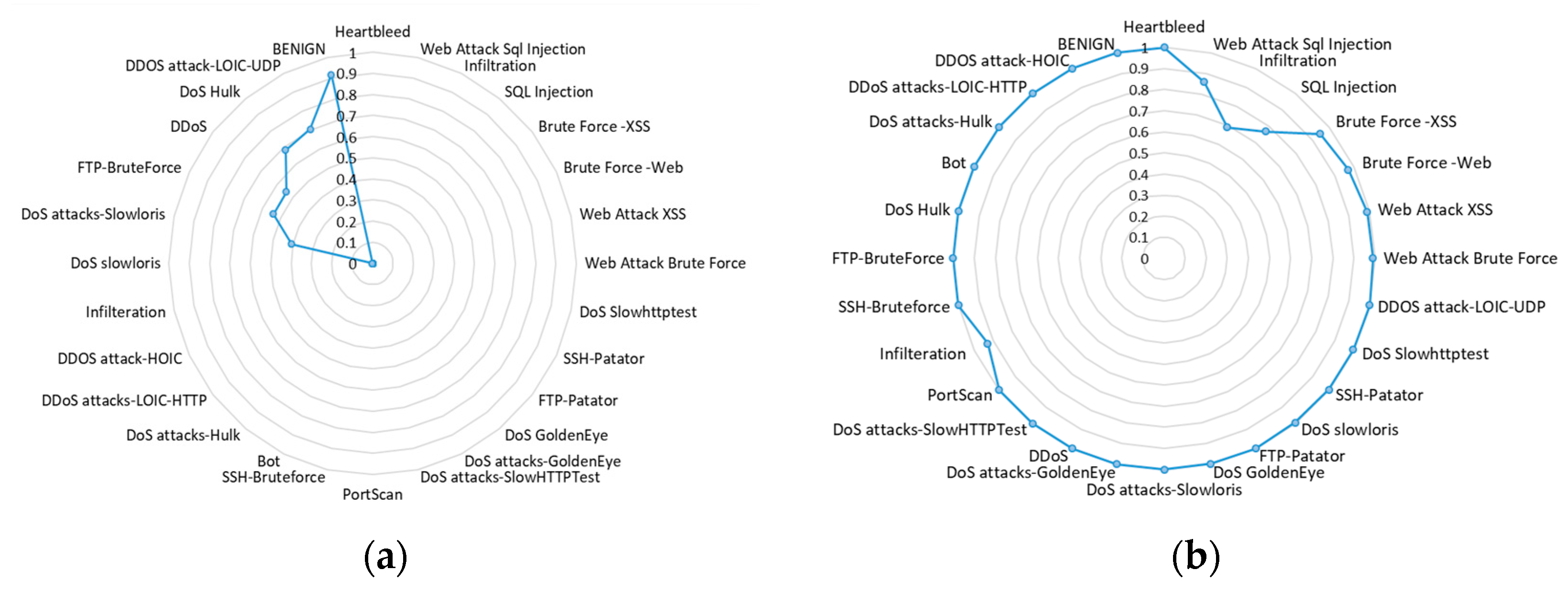
The F1-score accuracy results for each algorithm for each class of the dataset are presented below (see Figure 5). The figure shows that the LR model failed to detect such intrusion classes as “Bot”, “Heartbleed”, “Infiltration”, “PortScan”, “SSH-Patator” and “FTP -Patator”. F1-score values greater than 0 were obtained for such classes as “Dos slowloris” (0.18%), “DoS Attack-slowloris” (40.73%) and “DDoS” (54.25%), although these scores are not high. Higher values were obtained for only two classes—“Benign” (91.62%) and “DDOS attack-LOIC-UDP” (70.53%) (see Figure 5a). 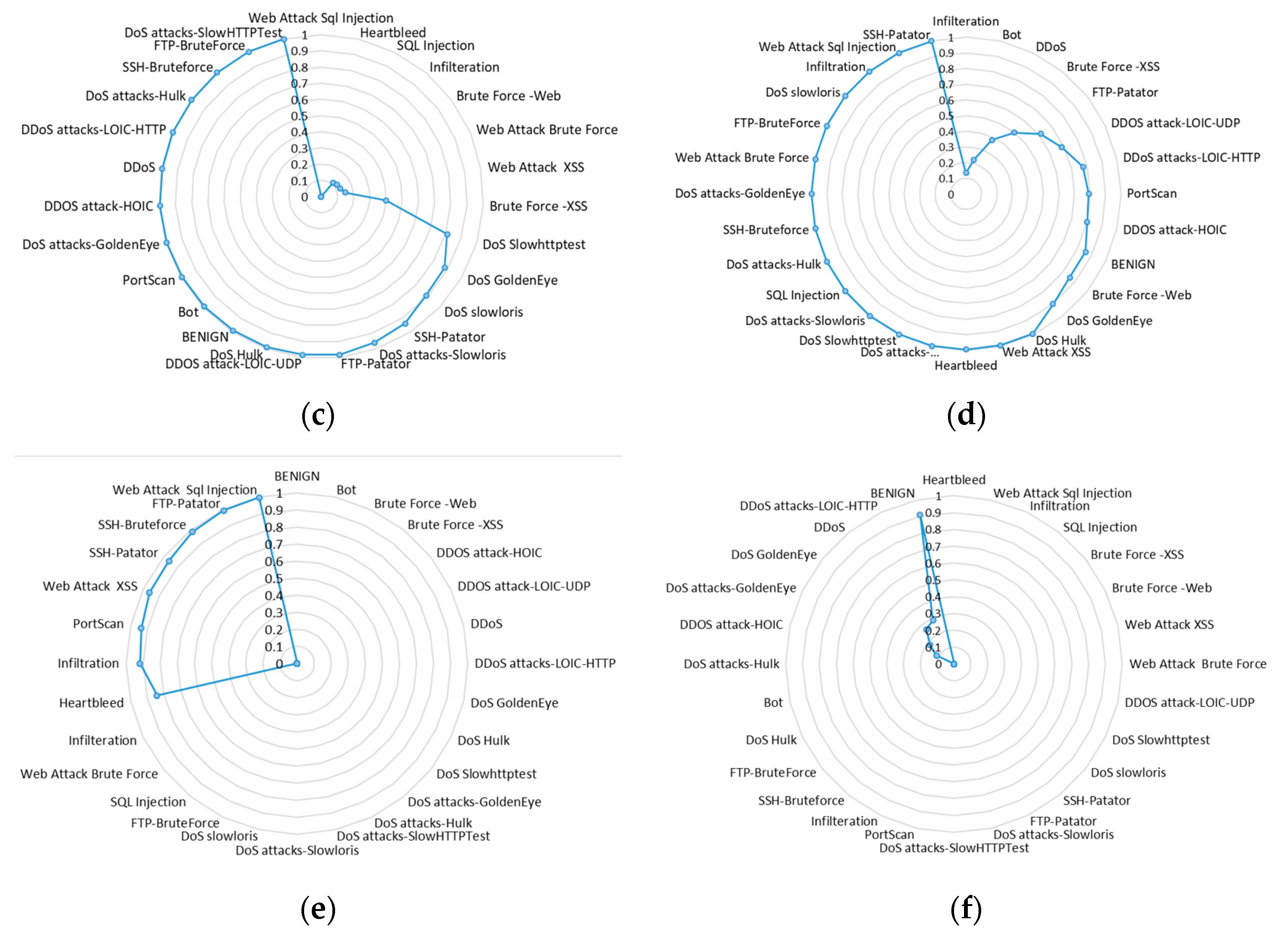The DT-based algorithms achieved quite high scores, but the most accurate was the DT(CART) algorithm, which reached high F1-score results (>90%) for the majority of classes (see Figure 5b). Only three attack classes had lower results: “Infiltration” (68.96%), “SQL Injection” (77.08%) and “Web Attack Sql Injection” (85.71%). The ID3 algorithm did not identify classes, such as “Web Attack Sql Injection”, “Heartbleed” and “SQL Injection”, but attacks, such as “SSH-Bruteforce”, “FTP-BruteForce” and “DoS attacks-SlowHTTPTest”, were identified with the highest accuracy >99.9% (see Figure 5c).

Concerning the results obtained from RF, the majority of classes were successfully classified with an accuracy rate exceeding 99%. Meanwhile, prediction success rates of “Web Attack-Brute Force”, “Web Attack-Sql Injection” and “Web Attack-XSS” data classes were significantly lower, ranging from 33.3% to 77.3%. Among the different data classes, the RF algorithm achieved the lowest score for “Infiltration” attacks (13.45%) and the highest score (99.99%) for “SSH-Patator” attacks, as illustrated in Figure 5d.

The classification results with MLP showed (Figure 5e) that the algorithm identified certain classes of attacks very well, i.e., “SSH-Bruteforce”, “FTP-Patator” and “Web Attack Sql Injection”, but did not identify others at all (the F1-score value was 0.). The worst results were obtained with the dense-layer net model, which only classified the “Benign” class correctly with 90.81% accuracy. Most intrusion attack classes had a classification accuracy of 0% value, and only a few had an accuracy in the range of 10–20% (“DDoS” type attacks).

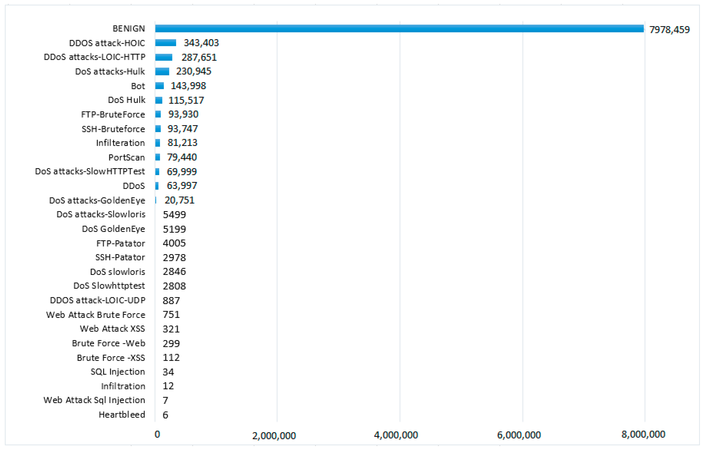
As the dataset was heavily imbalanced, it was important to verify how accuracy correlated with sample size. The testing sample size for each of the classes is given in Figure 6.

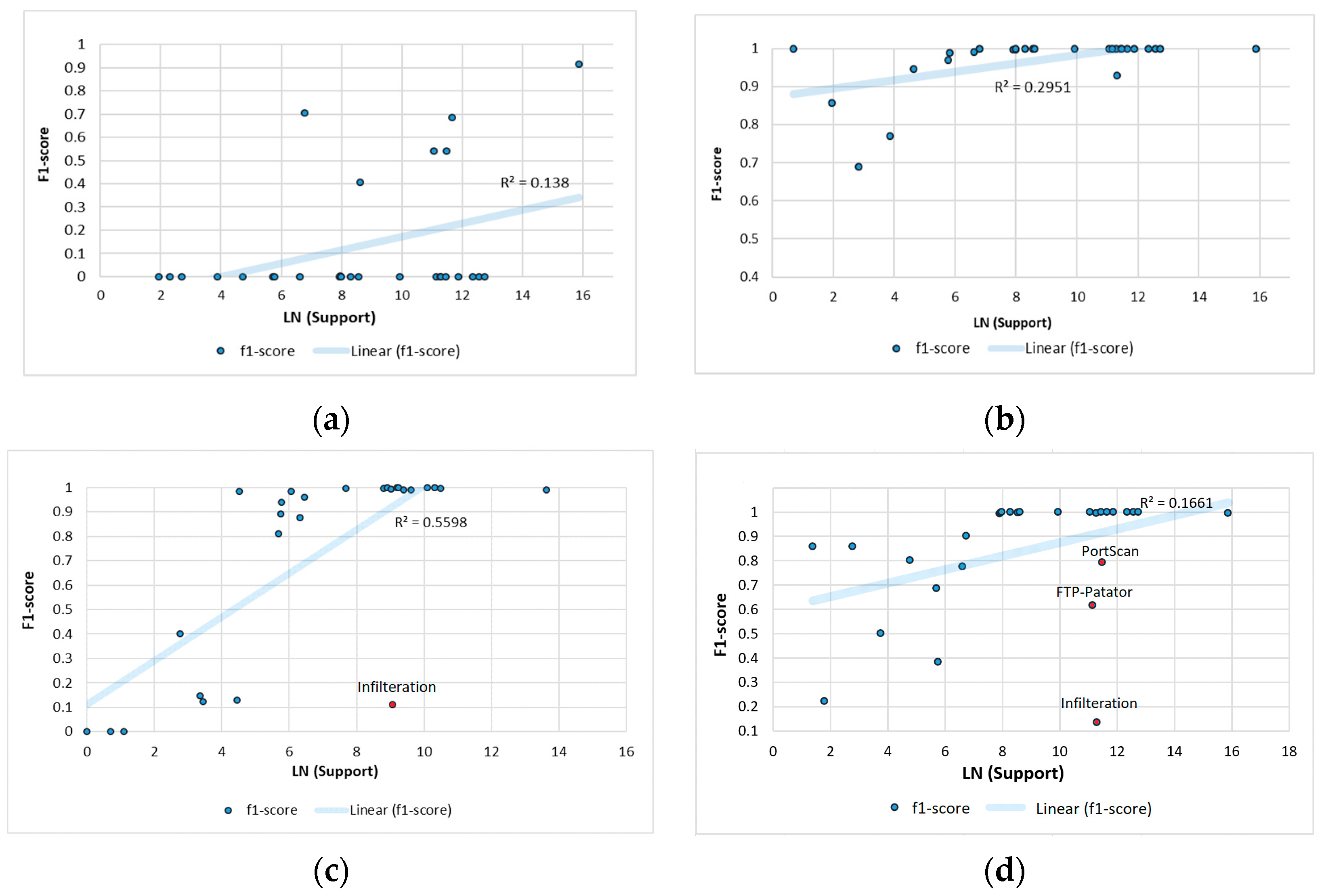
Support value dependencies on F1-score accuracy are provided in Figure 7. As the difference in support values was very significant, it was appropriate to consider a logarithmic scale for the support values. Near-linear dependencies were observed in the DT CART and ID3 models. However, the DT ID3 and RF models had more outliers. For example, the “Infilteration” class with a high support value only achieved 13.45% of F1-scores for the RF model and 11.09% for the DT ID3 model (see Figure 7c,d). Despite the low overall accuracy of the MLP model, the results presented in Figure 7e show that higher F1-scores were only obtained at higher values of support.

Figure 8 shows misclassification results for all six models, where it was important to evaluate the misclassification of malicious attacks as benign because this can lead to potential security risks and threats going undetected. Identifying and correctly classifying malicious attacks is important, but confusing certain malicious classes may be less critical than classifying them as benign. Figure 8 shows only malicious attacks, which are shown in red if the attack was correctly classified, in green if it was identified as benign and in gray if it was classified as malicious but the attack class was incorrectly assigned. The percentage values represented all of these cases for each attack class.

The lowest class confusion was observed for the DT CART model (see Figure 8c). Those attack classes with higher confusion had a very low number of samples, i.e., the number of samples used for testing ranged from 7 instances (“Web Attack Sql Injection”) to 100 (“Brute Force-XSS”). “Infiltration” attacks showed the most confusion, with 6 out of 17 attacks classified as “Benign” (green color) and 1 as another type (incorrect) of malware attack (gray color).

Comparing the DT ID3 algorithm and RF, we can see that the results were more satisfactory with RF because they classified less malicious attacks as benign. The worst situation was for “Infilteration” type attacks, as most of them were classified as benign (almost 90%) (see Figure 8d). The situation with regard to the classification of “Infilteration” attacks was the same as for the DT ID3 model (Figure 8b). In addition, more than 60% of the sample for the other seven types of attacks were also classified as benign. For the LR model (Figure 8a), we can see that the majority of malicious attacks were classified as benign (“Bot”, “Brute Force-Web”, “Heartbleed” “DoS GoldenEye”, etc.). The most inappropriate model was the dense-layer net, which classified almost all malicious attacks as benign. The MLP model identifyied at least seven types of malicious attacks with high accuracy, but the rest were classified as benign attacks (see Figure 8e).

6. XAI-Based Explanations

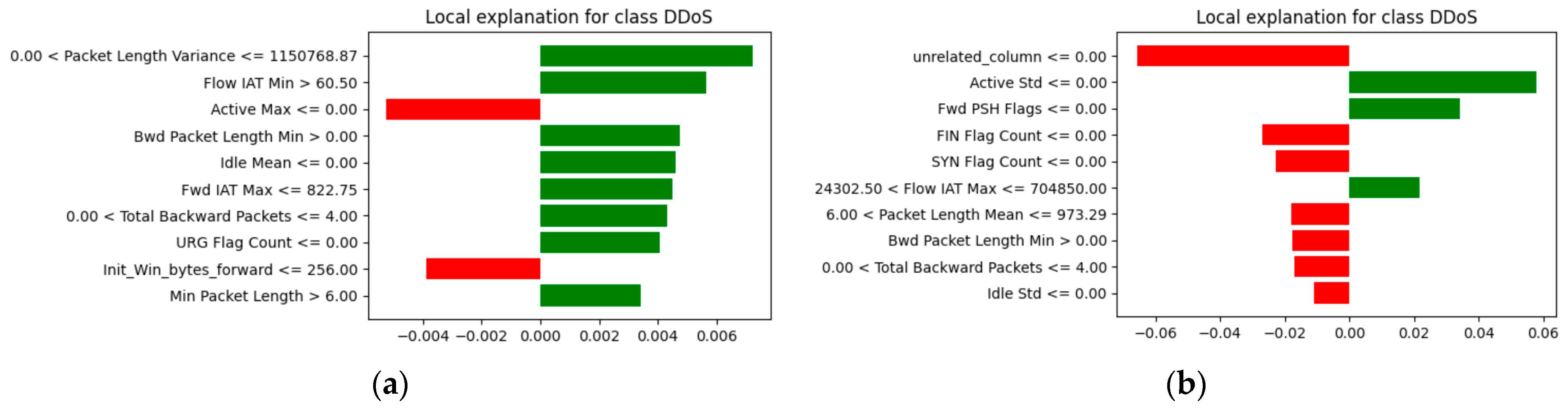
Experiments with two XAI methods—LIME and SHAP—were carried out to investigate their ability to explain classification results with more complex models, such as MLP. First, two multilayer perceptron models were created and trained on different datasets. The first model was trained with our joined CIC-IDS2017/-2018 dataset. The second model was trained with the same dataset, only with an addition of “unrelated_column” values, which were set randomly.

Both models’ explanations were first generated with LIME. For explanations, input values were selected that generated model predictions, indicating a network anomaly. In this case, inputs passed to both models indicated a network anomaly—“DDoS” attack.

Figure 9 shows which attributes had the greatest impact on the prediction, where the green columns indicate that they have a positive effect, i.e., they increase the model’s score, while the red columns decrease the score. From the data, it was observed that not only were the features that had the biggest impact on the model output different, but in “unrelated_column”, they had the most importance, although its values were completely random. However, in both cases, this instance was classified as a benign attack for the original dataset (see Figure 9a) with 83% probability and for the modified dataset (see Figure 9b) with 90% probability). Further explanations of both models were developed using the SHAP approach.

In this scenario, a sample instance of data had been submitted, the output of which was a “Benign” class. The data presented in Figure 10b shows that the results are similar to those of the LIME models, considering that “unrelated_column” had the largest impact on the decision.

When comparing the LIME and SHAP local explanation cases, almost every time the LIME explanations were generated, a different result was obtained, whereas SHAP was more stable in assessing the influence of attributes.

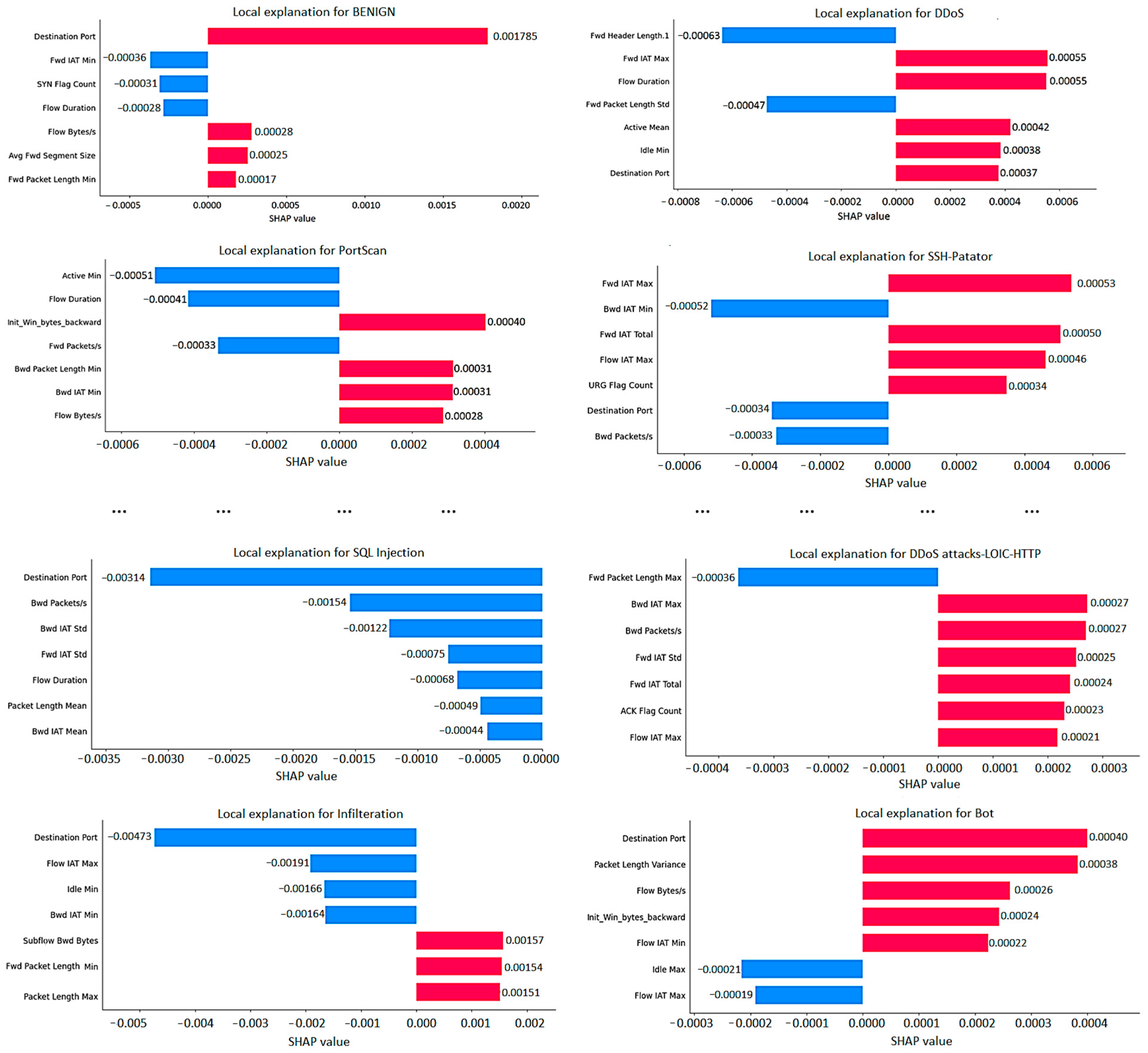
While performing the aforementioned experiments, certain drawbacks were observed of both LIME and SHAP explanation methods. For instance, LIME implementation is limited to providing explanations for individual instances within the dataset and lacks the ability to generate global explanations like SHAP. This means that in order to obtain a view of dataset-wide scope, the user has to generate explanations of every single instance of the dataset. Due to this issue, the process of analyzing and interpreting results can become complex, especially when working with datasets that contain over 19 million data entries, as is the case in our situation. Even in the case when a user is interested in only one data instance of the dataset, additional interpretability problems arise when a multiclass model is used. In this research, an MLP model was used to generate the LIME explanations, which resulted in separate explanations for all 28 classes, taking into account the influence of 79 features. The most interesting results for the eight classes are shown in Figure 11.

Meanwhile, SHAP can provide global explanations, and while this enables us to see explanations for the whole dataset, explanations can still be hard to interpret when using multiclass output models. Figure 12, provides global explanations for 28 classes, providing an importance score for the most dominant features. Although this allows for a detailed visualization of the explanation, the amount of data might be too confusing for the non-specialist end user.

7. Discussion

We conducted several experiments, varying the hyperparameters, to improve the accuracy of the best models in our investigation study. Regarding the CART tree, in the initial phase, the whole tree was generated to estimate its maximum size and performance. Subsequently, we carried out experiments by manipulating parameters, such as the maximum depth of the tree, the minimum number of samples required for a split, and the criteria (Gini impurity or entropy) used for splitting. During the initial stage, the CART tree achieved a maximum depth of 51 while utilizing a minimum of 2 samples as the criterion for node splitting and employing the “gini” criterion. To optimize the model’s performance, we applied pre-pruning techniques and limited the depth to 27. The decision was made to stop the growth of the tree at level 27 due to the observation that beyond this depth, there was confusion between the “BENIGN” class and the “Infiltration” class. Figure 8c provides further evidence of the significant confusion observed between these classes.

The ID3 algorithm, another DT algorithm employed in this study, initially generated a maximum depth of 48. Through experimentation, we progressively reduced the depth to 32, 25 and ultimately 19. Notably, a depth of 19 yielded the most accurate results. This stopping of the tree growth was appropriate because only the “BENIGN” and “Infilteration” classes were continuously mixed in the lower layers of the tree, which resulted in lower accuracy of the latter class (confusion with “BENIGN” reached 89.57%). Stopping the growth of the tree at a depth of 19 led to a minor enhancement in the accuracy, specifically for the “BENIGN” class, which already achieved high accuracy. However, the overall increase in the model’s accuracy remained relatively modest (1.04%). In addition, it was observed that splitting leaves with fewer than 6 elements was not very appropriate. However, considering the limited number of instances within certain specific classes of the dataset, such as “Heartbleed”, “SQL Injection” and “Web Attack SQL Injection”, the minimum number of instances required for splitting was adjusted to 3.

For the RF algorithm, we employed entropy criteria, which provided better results than “gini” in our case. We set the number of features to consider when searching for the optimal split as the square root of the total number of features (sqrt) provided in the dataset. The bootstrap method was utilized in our RF model; hence, out-of-bag samples were employed for estimating the generalization score. The number of trees in the forest was set to 100.

The observation reveals that conducting more comprehensive studies encompassing a wider range of hyperparameters would yield substantial benefits. Hence, we have intentions to persist with such studies in the future, as the results and insights will be crucial for the development of new XAI models.

Moreover, in this study, we carried out experiments using additional machine learning models, but only those models with the most promising practical results were selected for deeper analysis. As our future research goal is to develop robust and stable XAI models, it was necessary to test models with different levels of explainability (or interpretability) (see Figure 13). The accuracy results of the KNN model and LSTM are provided in

Table 4. Classification results of additional models.

Model	Performance Metrics	Precision	Recall	F1-Score
KNN	Accuracy	0.99399	0.99399	0.99399
	Weighted average	0.99367	0.99399	0.99342
	Macro average	0.81778	0.78565	0.79845
LSTM	Accuracy	0.89023	0.89023	0.89023
	Weighted average	0.83573	0.89029	0.85358
	Macro average	0.21564	0.19212	0.18313

. Throughout our experimentation, we explored different deep learning models, including VGG-19, AlexNet and several others. However, it was the LSTM model that gave the most accurate results. The main reason why these models were not included in the more detailed ones is the low average macro-level F1-score (<0.7).

KNN has fast learning capabilities; however, when it comes to making a decision, such as predicting a class based on new data, it takes much longer compared to the other machine learning algorithms implemented in our study. Therefore, we eliminated KNN as a real-time and practical algorithm, even though the accuracy rates obtained were actually very high (see Table 4), and it was the second best algorithm after CART.

8. Conclusions

This study addressed the challenges of understanding the results of multi-class classification of network intrusions in highly imbalanced data, including the CIC-IDS2017 and CSE-CIC-IDS-2018 datasets. In the research, machine learning models of different complexity and explainability were included in order to evaluate and understand whether more complex ML models were indeed capable of providing higher classification results for the classification of 28 classes of intrusions. The study compared the classification performance of six machine learning models using various measures of classification accuracy. The results revealed that the DT model utilizing the CART algorithm achieved the highest performance in the multi-class classification task, achieving an F1-score of 0.998 and an average macro F1-score of 0.969. The lowest results were obtained with the dense-layer network, with an F1-score of 0.833 and an average macro F1-score of 0.063. Another decision tree algorithm, namely ID3, along with the RF model, resulted in slightly lower but still significant results, achieving an F1-score of 0.985.

In addition, experiments were carried out with the XAI methods, LIME and SHAP, to assess the potential and reliability of identifying the most important features of the dataset. Although these methods provide a list of the most influential features, it has been observed that the local explanation is often unstable, and each regeneration may lead to a completely different result. Even a specially added column that has no relevance to the problem may have the greatest influence on the decision. Another observation is that a global interpretation of all classes is not very explicit, and it is quite difficult to understand the visualization. Therefore, it is likely that when we have more than multi-class and multi-feature datasets, it would be more useful to use numerical or aggregated results of explanations.