A Long-Term Traffic Flow Prediction Model Based on Variational Mode Decomposition and Auto-Correlation Mechanism

Abstract

Traffic flow forecasting, as an integral part of intelligent transportation systems, plays a critical part in traffic planning. Previous studies have primarily focused on short-term traffic flow prediction, paying insufficient attention to long-term prediction. In this study, we propose a hybrid model that utilizes variational mode decomposition (VMD) and the auto-correlation mechanism for long-term prediction. In view of the periodic and stochastic characteristics of traffic flow, VMD is able to decompose the data into intrinsic mode functions with different frequencies, which in turn helps the model extract the internal features of the data and better capture the changes of traffic flow data in the cycle. Additionally, we improve the residual structure by adding a convolutional layer to propose a correction module and use it together with the auto-correlation mechanism to jointly build an encoder and decoder to extract features from different data components (intrinsic mode functions) and fuse the extracted features for output. To meet the requirements of long-term forecasting, we set the traffic flow forecast length to 4 levels: 96, 192, 336, and 720. We validated our model using the departure statistics dataset of a taxi parking lot at Beijing Capital International Airport and achieved the best prediction performance in terms of mean squared error and mean absolute error, compared to the baseline model.

1. Introduction

With the development of intelligent transportation systems, sensor technology, computer technology, and other advanced technologies have found increasing applications in the field of transportation. However, these technologies are still insufficient to meet the demands of intelligent transportation development, and traffic congestion and accidents remain major issues that need to be addressed [1,2]. Traffic flow prediction, as a crucial component of intelligent transportation systems, can help with traffic light phase control, dynamic path planning for vehicle navigation, and other aspects that can reduce accidents, alleviate traffic congestion, and improve traffic conditions.

Over the years, traffic flow prediction methods have evolved with advancements in technology. The rapid development of sensing technology has made it easier to capture traffic flow data, providing a more substantial dataset for forecasting purposes [3,4,5,6]. Traffic flow data are often obtained through video detection, microwave sensors, etc. Traffic flow, as time series data, tends to show a predictable pattern of change within a day. However, factors such as holidays and weather can cause fluctuations and changes in traffic flow, making it challenging to predict accurately. In the past, autoregressive integrated moving average (ARIMA) models were commonly used for traffic flow prediction due to their simplicity and effectiveness [7,8,9]. However, these models are unable to capture the nonlinear features present in traffic flow, resulting in mediocre prediction performance. Similar problems also lie in the support vector regression (SVR) and k-nearest neighbors (KNN) models. With the development of deep learning, convolutional-neural-network-based prediction methods [10] and recurrent-neural-network-based prediction methods [11,12] have been employed for traffic flow prediction. These models are capable of extracting internal features of traffic flow and grasping the traffic flow change pattern more effectively than previous methods, achieving good results in short-term traffic flow prediction. In particular, LSTM [11] neural network is widely used in short-term traffic flow prediction but may not be suitable for long series prediction. The introduction of transformer [13] has led to widespread attention on self-attention, resulting in numerous models derived on this basis for long series prediction, providing new ideas for the development of our traffic flow prediction.

Adequate and effective data features are key to improving the accuracy of prediction models. To delve deeper into the internal change patterns of traffic flow data and enhance the model’s ability to extract data features, some researchers have utilized data decomposition methods to assist prediction models for time series prediction, such as wavelet decomposition and empirical mode decomposition (EMD) [14], which have achieved better prediction results than single models. However, while wavelet decomposition is less adaptive, EMD and its improved algorithms suffer from endpoint effects and over-envelope problems. Variational mode decomposition (VMD) [15] is an adaptive, fully recursive modal variational method that can address these issues and more effectively decompose single traffic flow data into multiple components with different frequencies. This facilitates the model to fully extract the internal features of the data and achieve more accurate prediction results. Given VMD’s excellent data decomposition ability and the auto-correlation mechanism’s advantage for long-term prediction, we developed a sequence-to-sequence hybrid model for traffic flow prediction. Our main contributions are threefold: first, for traffic flow forecasting, where previous studies have focused on short-time traffic flow forecasting, we performed long-term forecasting; second, we constructed a hybrid model using VMD and auto-correlation mechanism, and improved the residual structure by adding a convolutional layer to propose a correction module that enhances the robustness of the model; and third, we tested our model using real datasets and achieved the best measured results compared to other baseline models.

We provide detailed reviews of previous research in traffic flow prediction in Section 2. In Section 3, we introduce VMD, auto-correlation mechanism, and the correction module, build the encoder and decoder, and construct our hybrid model. Experimental validation is conducted in Section 4. In Section 5, we summarize the research in this paper and provide an outlook on the future development of traffic flow.

2. Related Work

Traffic flow prediction plays a crucial role in traffic management and transportation planning. Accurate prediction of traffic flow can help to alleviate congestion, reduce travel time, and improve safety. Currently, machine learning is widely used in the field of traffic flow prediction and there are many models [16,17,18]. Zhang Ning et al. [19] used a particle swarm optimization algorithm to find the key parameters in the SVM, and then improved the prediction accuracy of short-term traffic flow. Cai Lingru et al. [20] proposed a KNN regression model for short-term traffic flow prediction by optimizing the traditional KNN regression algorithm. The model restructures the balanced training set to address the data imbalance issue in traffic flow data and considers the local and global patterns of traffic flow data. In addition to regression algorithms, with the development of deep learning, Zhao Wentian et al. [21] used a TCN model for traffic flow prediction, and this convolutional model greatly improves the parallelization of traffic data operation. Although the above models can also achieve traffic flow prediction, the prediction accuracy is slightly poor, and furthermore, more scholars use long- and short-term memory networks to build hybrid prediction models. In 2019, Yang Bailin et al. [22] used the LSTM model as the basis and added the attention mechanism to better predict traffic flow data. Ahmad Ali et al. [23] combined CNN, LSTM, and attention mechanism, and proposed ATT-DHSTNet network architecture, which gave full play to the extraction ability of convolutional network for spatial information and recurrent neural network for temporal information, together with the control of global information by attention mechanism; this achieved good prediction results. Luo Xianglong et al. [24] used the KNN algorithm for spatial location site selection, considering the influence relationship between the traffic volumes of different location sites; then, the traffic volumes of different sites were predicted separately using the model built by the LSTM module; and finally the traffic predictions between different sites were given different weights as the predicted value of the site.

Recurrent neural networks (RNNs) have been widely used in traffic flow prediction due to their high accuracy [25,26,27,28]. However, recurrent neural networks suffer from gradient disappearance and gradient explosion, and the prediction accuracy decreases dramatically as the prediction length increases. To address this issue, researchers have explored methods such as self-attention mechanism to achieve long-term time series prediction. In recent years, many scholars have proposed various models based on self-attention mechanism, including Zhou Haoyi et al.’s informer model [29], Wu Haixu et al.’s autoformer model [30], and Zhou Tian’s FEDformer model [31]. The informer model, developed on the basis of the transformer model for time series forecasting, applies self-attention mechanism to acquire similarity information for individual data points without considering the whole sequence. The autoformer model proposes an auto-correlation mechanism, in which the time-delayed aggregation operation further considers both individual and overall information and presents better results in traffic flow prediction. The FEDformer model predicts traffic flow from the perspective of the frequency domain. Compared with traditional RNNs, these models—based on self-attention mechanism—show better prediction performance in multi-step prediction.

Due to the common characteristics of nonlinearity, stochasticity and instability of time series data such as stock prices, wind power generation, water flow, and traffic flow, the data decomposition methods used in other fields can be applied to traffic flow data to improve prediction accuracy. For instance, Hao Wei et al. combined EMD and LSTM models to mitigate the nonlinearity and non-smoothness of traffic flow data using EMD and formed a hybrid model [32]. Li Yiqun et al. utilized wavelet decomposition to smooth the data, which is beneficial for the model to extract long-term relational features [33]. Compared with wavelet decomposition and EMD, VMD can better solve the problems of modal mixing and frequency adaptation, which is beneficial for the model prediction accuracy. Several studies have demonstrated that VMD has a more significant enhancement effect on prediction compared to other methods [34,35,36,37]. Bing Qichun et al. [38] employed VMD to decompose traffic flow data into different modal components, extracted features from each modal component using an LSTM model, and achieved multi-step prediction by accumulating the predicted values of previous steps. Liu Hui et al. [39] converted traffic flow data into different frequency components using VMD, optimized weights using ICA algorithm, and integrated three prediction models (GMDH, BILSTM, and ELMAN) to predict different modal components. Tang Jingwei et al. [40] decomposed environmental variables using VMD and found the most power-relevant modal components based on MIC and Pearson correlation coefficients, predicting them along with historical power data. Cai Changchun et al. [41] utilized GRU models to achieve prediction of low frequency components and TCN models to achieve prediction of high frequency components after VMD modal decomposition. Finally, they reconstructed the prediction results of low and high frequency data as final prediction values. Overall, hybrid models formed by combining data decomposition methods and prediction models generally achieve good prediction results in traffic flow prediction.

3. Model Structure

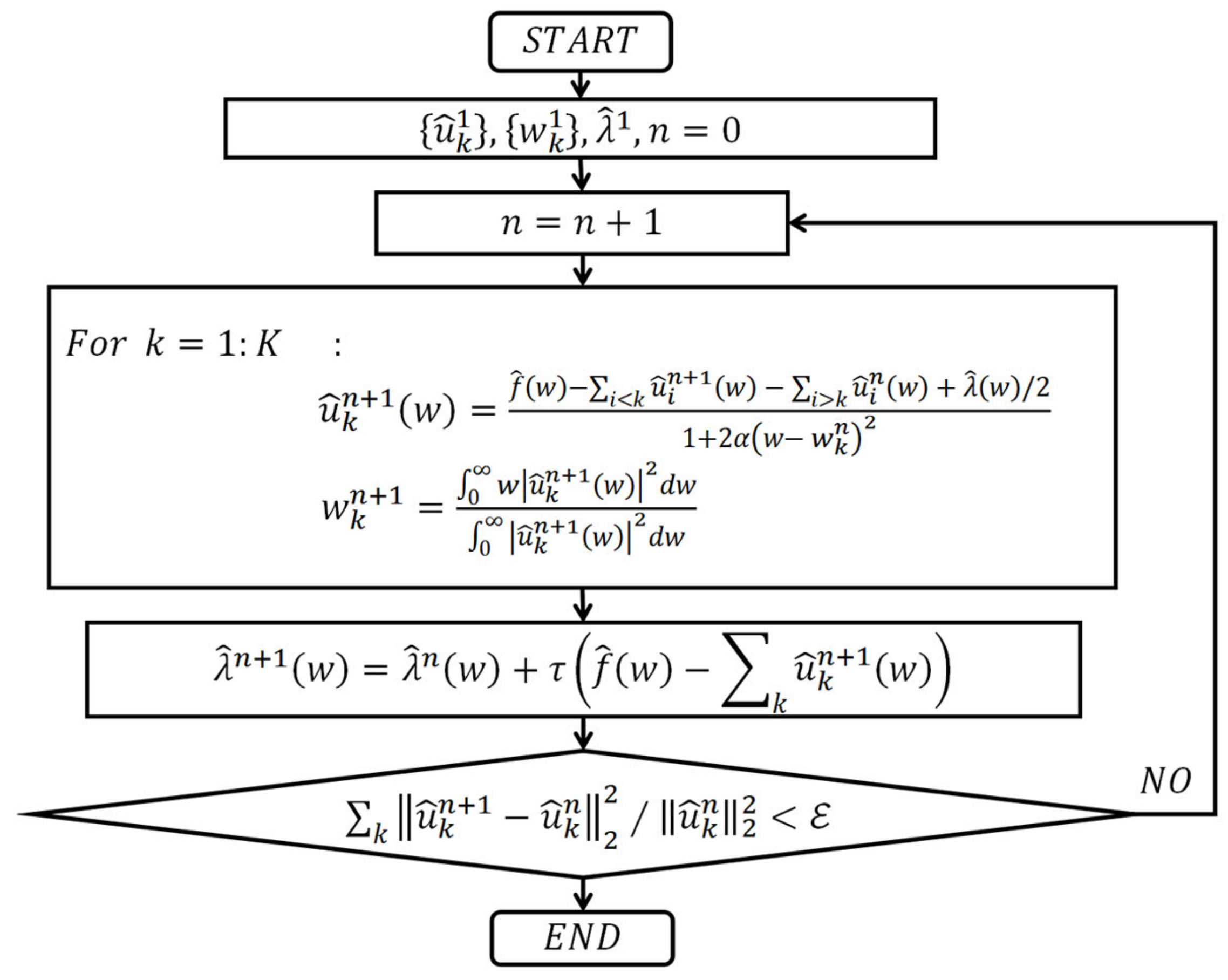
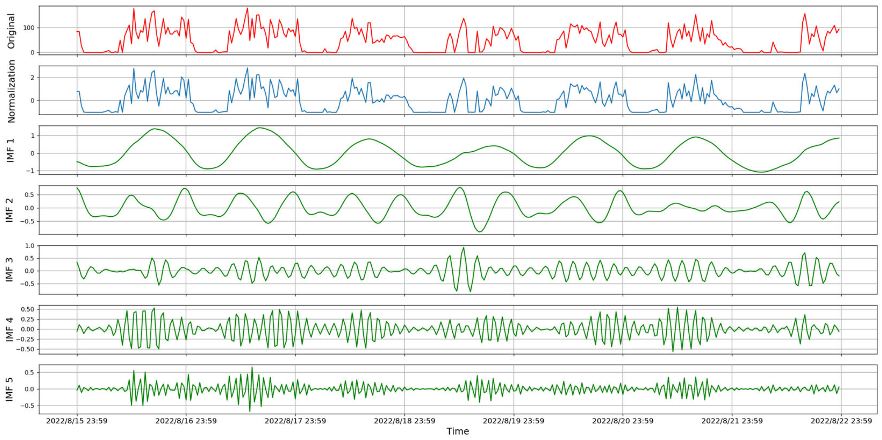
3.1. Variational Mode Decomposition

Variational mode decomposition (VMD) [15] decomposes time series data f into K intrinsic mode functions (IMFs) of different frequencies, ${\mathrm{u}}^{\mathrm{k}}$; each ${\mathrm{u}}^{\mathrm{k}}$ corresponds to a central frequency, ${\mathrm{w}}^{\mathrm{k}}$. To evaluate the broadband of ${\mathrm{u}}^{\mathrm{k}}$, the constrained variational problem follows, as follows:

$$\begin{gathered} \begin{array}{c}\min \\ \left\{{\mathrm{u}}^{\mathrm{k}}\right\},\left\{{\mathrm{w}}^{\mathrm{k}}\right\}\end{array}=\left\{{{\displaystyle \sum }}_{\mathrm{k}}\Vert {\partial }_{\mathrm{t}}\left[\left(\mathsf{\delta }\left(\mathrm{t}\right)+\frac{\mathrm{j}}{\mathsf{\pi }\mathrm{t}}\right){ \ast \mathrm{u}}_{\mathrm{k}}\left(\mathrm{t}\right)\right]{\mathrm{e}}^{-{\mathrm{jw}}_{\mathrm{k}}\mathrm{t}}{\Vert }_2^2\right\}, \\ \mathrm{s}.\mathrm{t}. {{\displaystyle \sum }}_{\mathrm{k}}{\mathrm{u}}_{\mathrm{k}}=\mathrm{f}. \end{gathered}$$

(1)

In the above equations,$\left\{{\mathrm{u}}_{\mathrm{k}}\right\}:=\left\{{\mathrm{u}}_1,{\mathrm{u}}_2,\dots {\mathrm{u}}_{\mathrm{K}}\right\}$ and $\left\{{\mathrm{w}}_{\mathrm{k}}\right\}:=\left\{{\mathrm{w}}_1,{\mathrm{w}}_2,\dots {\mathrm{w}}_{\mathrm{K}}\right\}$ denote all modes and their corresponding central frequencies, respectively. ${\partial }_{\mathrm{t}}$ denotes the differential processing of t, $\Vert ·\Vert$ denotes the norm processing, ${\mathsf{\delta }}_{\mathrm{t}}$ denotes the Dirca function, * is the convolution symbol, and ${\displaystyle \sum }_{\mathrm{k}}:={{\displaystyle \sum }}_{\mathrm{k}=1}^{\mathrm{K}}$ represents the sum of all modes.

In order to transform the problem constrained to unconstrained, an augmented Lagrangian function L is introduced:

$$\begin{gathered} \mathrm{L}\left(\left\{{\mathrm{u}}_{\mathrm{k}}\right\},\left\{{\mathrm{w}}_{\mathrm{k}}\right\},\mathrm{\lambda }\right)=\mathsf{\alpha }{{\displaystyle \sum }}_{\mathrm{k}}\Vert {\partial }_{\mathrm{t}}\left[\left(\mathsf{\delta }\left(\mathrm{t}\right)+\frac{\mathrm{j}}{\mathsf{\pi }\mathrm{t}}\right){ \ast \mathrm{u}}_{\mathrm{k}}\left(\mathrm{t}\right)\right]{\mathrm{e}}^{-{\mathrm{jw}}_{\mathrm{k}}\mathrm{t}}{\Vert }_2^2+||\mathrm{f}\left(\mathrm{t}\right)-{{\displaystyle \sum }}_{\mathrm{k}}{\mathrm{u}}_{\mathrm{k}}\left(\mathrm{t}\right){\left|\right|}_2^2+ \\ \langle \mathrm{\lambda }\left(\mathrm{t}\right), \mathrm{f}\left(\mathrm{t}\right)-{{\displaystyle \sum }}_{\mathrm{k}}{\mathrm{u}}_{\mathrm{k}}\left(\mathrm{t}\right)\rangle , \end{gathered}$$

(2)

where $\mathsf{\alpha }$ is the penalty factor and $\mathrm{\lambda }\left(\mathrm{t}\right)$ is the Lagrangian multiplier. The IMF component ${\mathrm{u}}_{\mathrm{k}}$ and the central frequency ${\mathrm{w}}_{\mathrm{k}}$ of each mode are updated according to the alternate direction method of multipliers. The complete algorithm flow of the variational mode decomposition is shown in Figure 1.

3.2. Auto-Correlation Mechanism and Correction Module

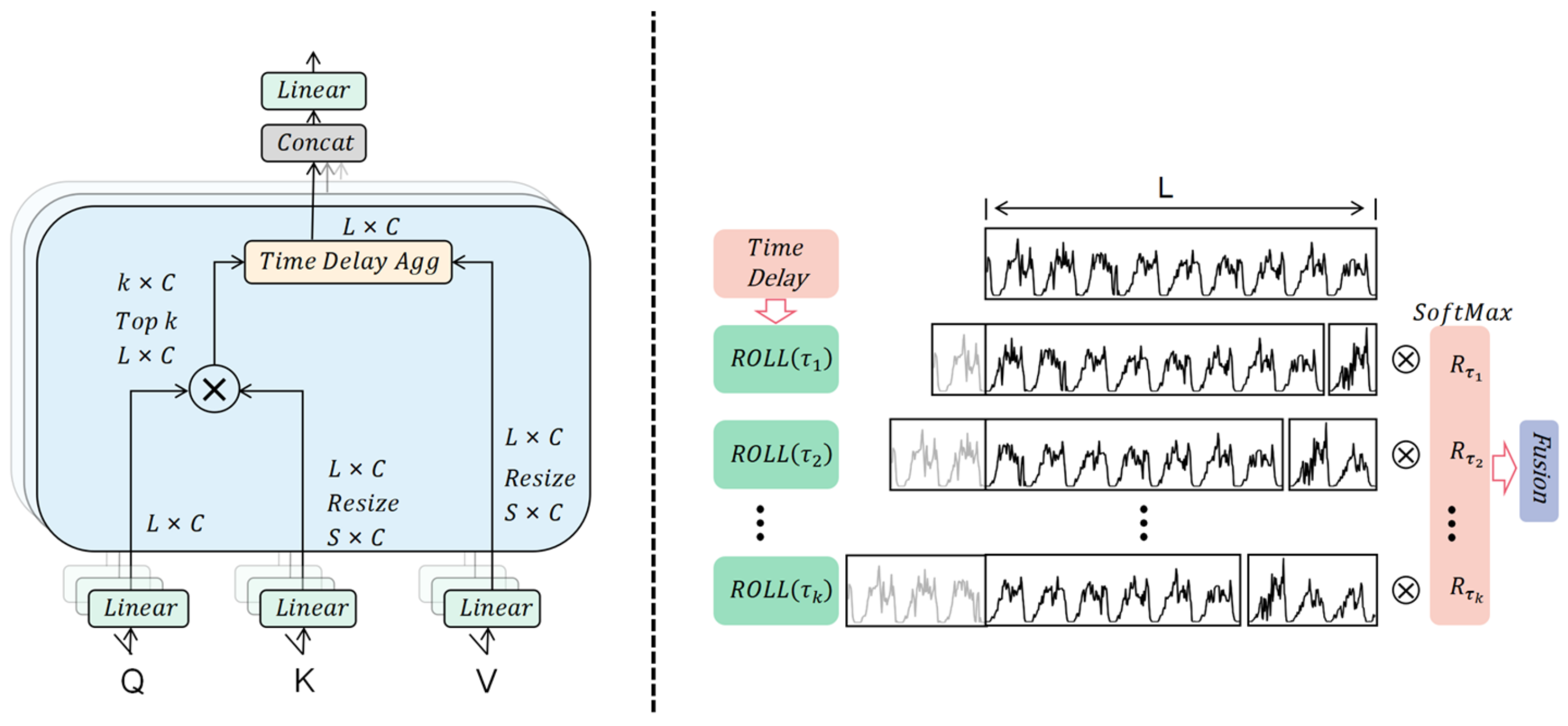
3.2.1. Auto-Correlation Mechanism

We are inspired to calculate the similarity of query and key by the following formula based on the use of Fourier transform in autoformer [30].

$${\mathrm{R}}_{\mathrm{Q},\mathrm{K}}=\mathrm{QK}.$$

(3)

The R_Q,K represents the similarity {Q} to sequence {K} as the weight for calculating attention.

As shown in Figure 2, the auto-correlation mechanism [30] uses sequences with high similarity to calculate auto-correlation, discarding sequences with poor similarity, which reduces the computational effort while ensuring the computational accuracy. The time delay aggregation block is the core of the auto-correlation mechanism, and the detailed steps in the single-head auto-correlation mechanism are as follows.

$$\begin{gathered} \begin{array}{c}{\mathsf{\tau }}_1,\dots ,{\mathsf{\tau }}_{\mathrm{k}}=\mathrm{argTopk}\left({\mathrm{R}}_{\mathrm{Q},\mathrm{K}}\left(\mathsf{\tau }\right)\right)\\ \mathsf{\tau }ϵ\left\{1,\dots ,\mathrm{L}\right\}\end{array}, \\ {\hat{\mathrm{R}}}_{\mathrm{Q},\mathrm{K}}\left({\mathsf{\tau }}_1\right),\dots ,{\hat{\mathrm{R}}}_{\mathrm{Q},\mathrm{K}}\left({\mathsf{\tau }}_{\mathrm{k}}\right)=\mathrm{SoftMax}\left({\mathrm{R}}_{\mathrm{Q},\mathrm{K}}\left({\mathsf{\tau }}_1\right),\dots ,{\mathrm{R}}_{\mathrm{Q},\mathrm{K}}\left({\mathsf{\tau }}_{\mathrm{k}}\right)\right), \\ \mathrm{Auto}-\mathrm{Correlation}\left(\mathrm{Q},\mathrm{K},\mathrm{V}\right)={{\displaystyle \sum }}_{\mathrm{i}=1}^{\mathrm{k}}\mathrm{Roll}\left(\mathrm{V},{\mathsf{\tau }}_{\mathrm{i}}\right){\hat{\mathrm{R}}}_{\mathrm{Q},\mathrm{K}}\left({\mathsf{\tau }}_{\mathrm{i}}\right). \end{gathered}$$

(4)

In the above equation, L represents the sequence length of key and value, k = 10 c, ${\hat{\mathrm{R}}}_{\mathrm{Q},\mathrm{K}}$ is the auto correlation of ${\mathrm{R}}_{\mathrm{Q},\mathrm{K}}$ after the operation of $\mathrm{SoftMax}$ normalization. $\mathrm{Roll}\left(\mathrm{V},{\mathsf{\tau }}_{\mathrm{i}}\right)$ serves to delay the value of V by ${\mathsf{\tau }}_{\mathrm{i}}$ steps.

The multi-head auto-correlation mechanism can parallelize the operations of the single-head auto-correlation mechanism and play a better prediction effect, and we use the multi-head auto-correlation mechanism with the following formula. In the multi-head auto-correlation mechanism, ${\mathrm{W}}_{\mathrm{output}}$ is a linear mapping parameter, the number of channels of the hidden variable is $\mathrm{d}\_\mathrm{model}$, the number of heads is $\mathrm{h}$, and the query, key, and value values of the i-th head are ${\mathrm{Q}}_{\mathrm{i}},{\mathrm{K}}_{\mathrm{i}},{\mathrm{V}}_{\mathrm{i}}ϵ{ℝ}^{\mathrm{L}\times \frac{\mathrm{d}\_\mathrm{model}}{\mathrm{h}}}$, $\mathrm{i}\in \left\{1,\dots ,\mathrm{h}\right\}$.

$$\begin{gathered} \mathrm{Multihead}\left(\mathrm{Q},\mathrm{K},\mathrm{V}\right)={\mathrm{W}}_{\mathrm{output}} \ast \mathrm{Concat}\left({\mathrm{head}}_1,\dots ,{\mathrm{head}}_{\mathrm{h}}\right), \\ {\mathrm{where} \mathrm{head}}_{\mathrm{i}}=\mathrm{Auto}-\mathrm{Correlation}\left({\mathrm{Q}}_{\mathrm{i}},{\mathrm{K}}_{\mathrm{i}},{\mathrm{V}}_{\mathrm{i}}\right). \end{gathered}$$

(5)

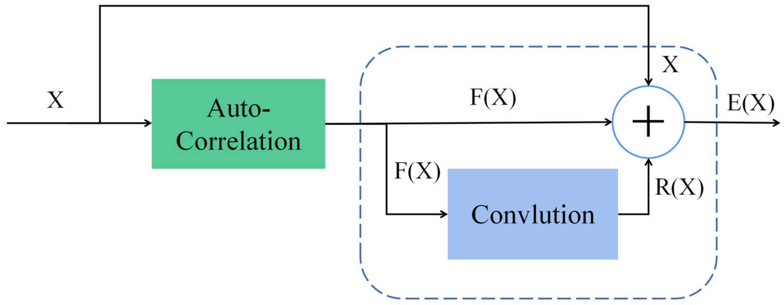
3.2.2. Correction Module

The correction module is improved on the basis of residual structure. In deep learning research, many scholars adopt the residual structure to protect the integrity of data and mitigate the gradient disappearance problem; additionally, some scholars also adopt the convolution method for time series prediction. Inspired by this, we perform the convolution operation on the features extracted by the auto-correlation mechanism as new features to be added to the results of the residual structure; the steps are shown in Figure 3. The correction module complements and optimizes the residual structure, the process of which can be defined as:

$$\begin{gathered} \mathrm{R}\left(\mathrm{X}\right)=\mathrm{Conv}\left(\mathrm{F}\left(\mathrm{X}\right)\right), \\ \mathrm{E}\left(\mathrm{X}\right)=\mathrm{F}\left(\mathrm{X}\right)+\mathrm{X}+\mathrm{R}\left(\mathrm{X}\right). \end{gathered}$$

(6)

In the above equation, X represents the data variable before entering the auto-correlation mechanism, and F(X) represents the output after the operation of the auto-correlation mechanism. R(X) is the result of convolution of F(X); X,F(X) and R(X) are added together to obtain E(X) as the output of the correction module.

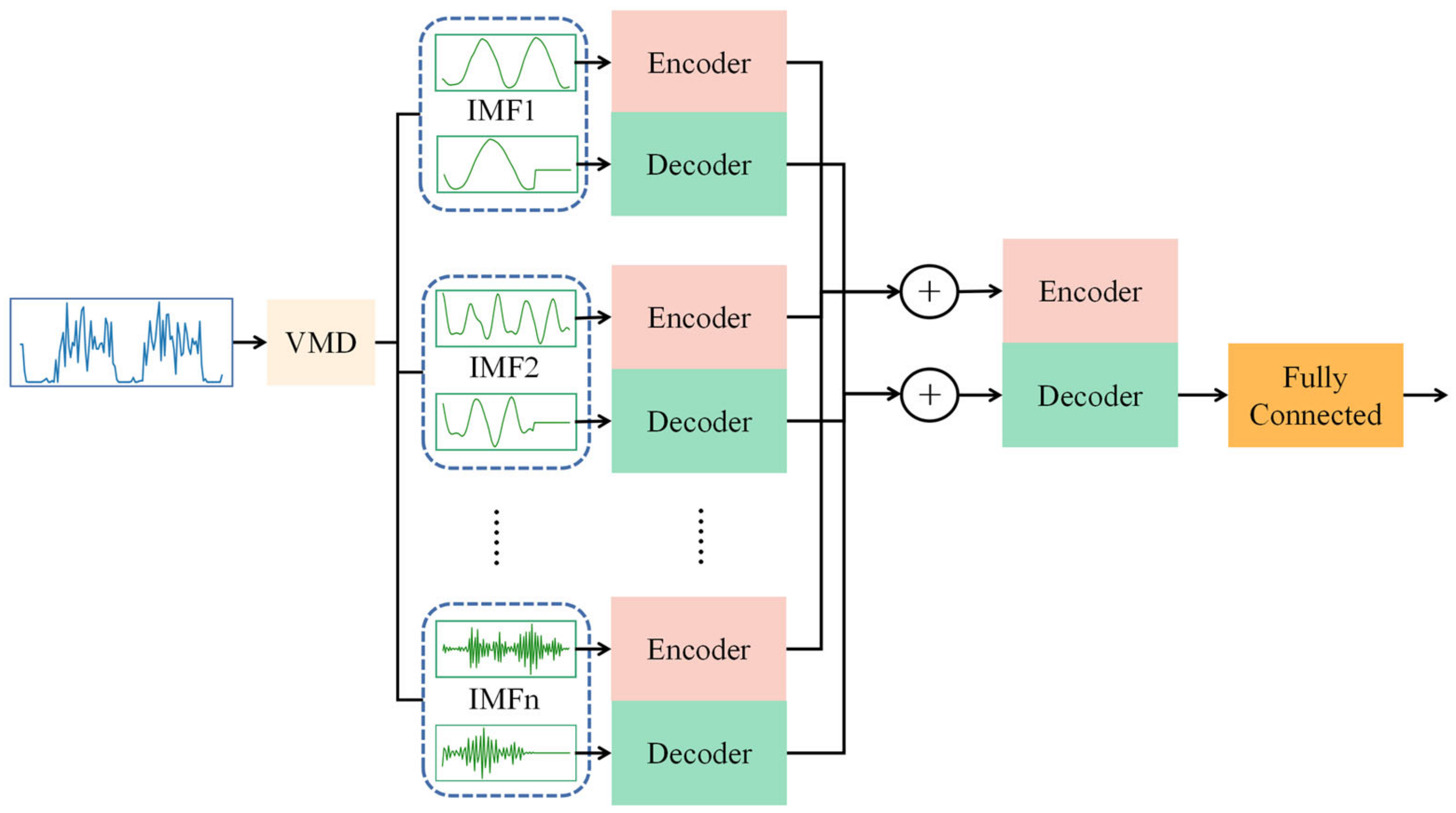
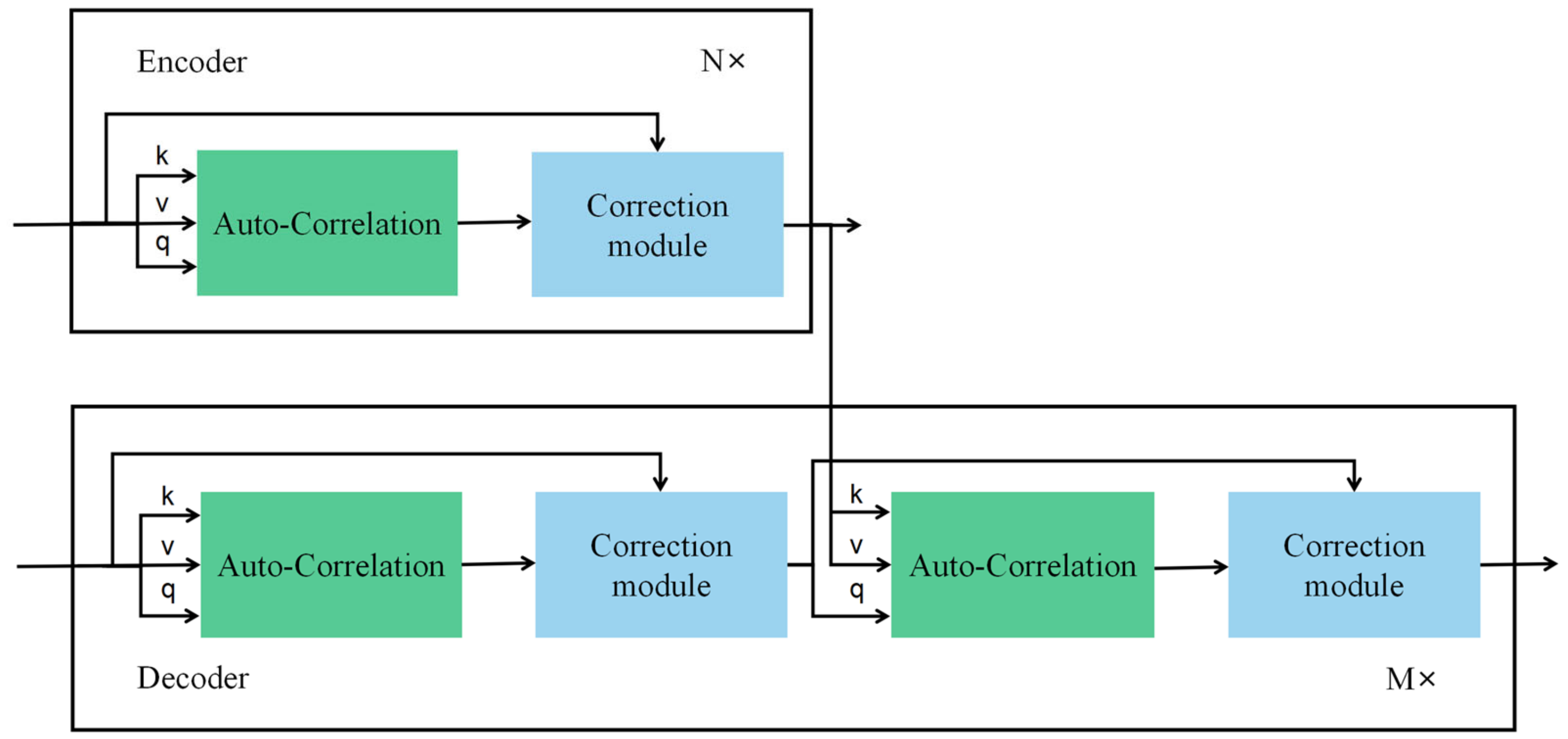
3.3. Model Framework

Our model consists of variational mode decomposition, auto-correlation mechanism and correction module, and its model structure is shown in Figure 4. By variational mode decomposition, multiple intrinsic mode functions with different frequencies and the same length can be obtained. Each intrinsic mode function corresponds to an encoder and decoder, respectively, and the detailed internal structure of the encoder and decoder is shown in Figure 5. The encoding and decoding operations for data of different frequencies can not only reduce the data noise, but also analyze the patterns of data changes more carefully and comprehensively, and then extract more useful data information. The calculation results of the encoder for each intrinsic mode function are added together as the final input for encoding, and the output of the decoder for each Intrinsic mode function is added together as the final input for decoding so that the extracted data information from different frequencies can be fully integrated. Finally, the desired predicted output length is obtained through linear mapping.

In the encoder and decoder, we compute auto correlation for all the sequence data on the input, increasing the efficiency of using all the data. The data integrity are further enhanced by the correction module after the output of the auto-correlation mechanism.

Our encoder consists of N stacks of identical layers. Each layer contains only one auto-correlation mechanism and correction module; the data are computed by the auto-correlation mechanism and correction module; and then, the layer normalization operation is performed, and this cycle is carried out until the key and value are output. Our decoder is composed of M stacks of identical layers. Each layer also contains only an auto-correlation mechanism and a correction module. The key and value from the encoder operate with the auto-correlation mechanism with the new input query, and then use the correction module to correct the data, and finally also perform the layer normalization operation, and so on until the auto correlation value is output.

4. Experiment and Analysis

4.1. Experimental Data and Evaluation Indexes

We use the dataset called BCAT to validate the performance of our model. The important information of BCAT is shown in

Table 1. Description of BCAT.

Dataset	Time	Acquisition Frequency	Total Number	Splitting Strategy
				Train Validation Test
BACT	15 August 2022–31 December 2022	30 min	6600	0–3960	3960–5280	5280–6600

. BCAT is a taxi parking lot departure statistical dataset from Beijing Capital International Airport. The statistics interface counts the number of taxi departures from the parking lot every half hour. BCAT records the departure data of the terminal taxi parking lot from 15 August 2022 to 31 December 2022, with a total of 6600 entries. We standardized the original data, and then decomposed the original data into modal components with different frequencies by using the VMD method. We verified several times that the center frequency of the last modal data tends to be smooth when the decomposition number K is equal to 5. As shown in

Table 2. The center frequency of IMF at different K.

K	IMF1	IMF2	IMF3	IMF4	IMF5	IMF6	IMF7	IMF8
2	0.02011	0.25129
3	0.01700	0.04149	0.33699
4	0.01844	0.04184	0.25042	0.33892
5	0.01845	0.10044	0.17884	0.26595	0.41738
6	0.01788	0.04046	0.10638	0.25459	0.33735	0.42155
7	0.02001	0.03570	0.06523	0.18236	0.25355	0.33450	0.42184
8	0.01869	0.03885	0.10596	0.18952	0.27130	0.32840	0.37020	0.43156

, when the decomposition number is less than 5, the last central frequency decreases, indicating that there may be hidden information not unearthed; when the decomposition number is greater than 5, there are similarities between the modes, leading to modal duplication. Therefore, we set the decomposition number K to 5. Part of the original data, the data after standardization and the imfs after the variational modal decomposition are shown in Figure 6. We divided the BCAT dataset into training set, validation set, and test set with the ratio of 6:2:2.

We use mean square error (MSE) and mean absolute error (MAE) to verify the performance of the model, with smaller values of both metrics indicating better model prediction performance. These two indicators can be defined as:

$$\begin{gathered} \mathrm{MSE}=\frac{1}{\mathrm{n}}{{\displaystyle \sum }}_{\mathrm{t}=1}^{\mathrm{n}}{\left({\mathrm{y}}_{\mathrm{t}}-{\hat{\mathrm{y}}}_{\mathrm{t}}\right)}^2, \\ \mathrm{MAE}=\frac{1}{\mathrm{n}}{{\displaystyle \sum }}_{\mathrm{t}=1}^{\mathrm{n}}\left|{\mathrm{y}}_{\mathrm{t}}-{\hat{\mathrm{y}}}_{\mathrm{t}}\right|. \end{gathered}$$

(7)

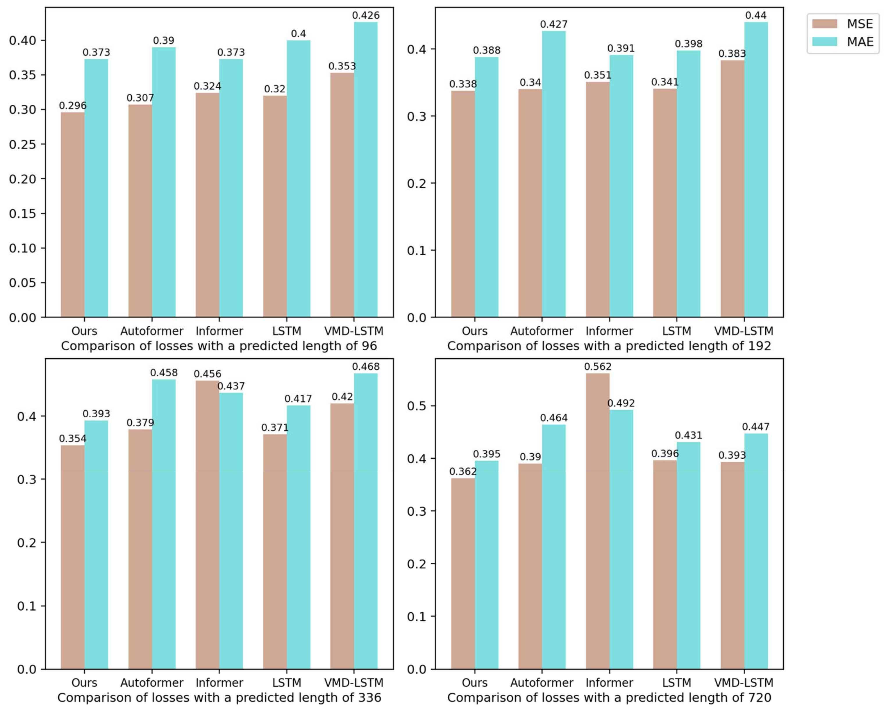
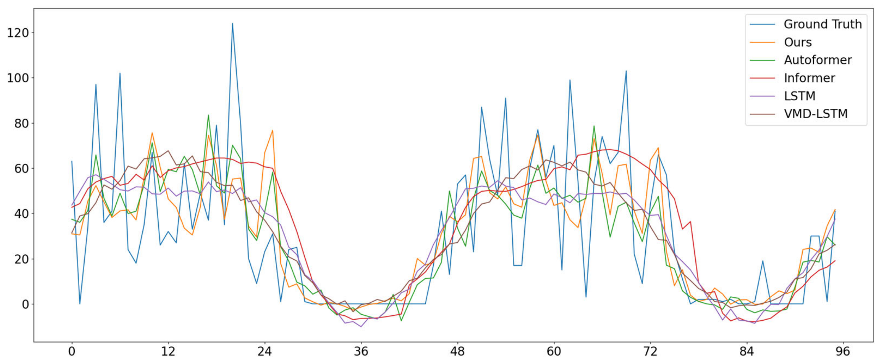
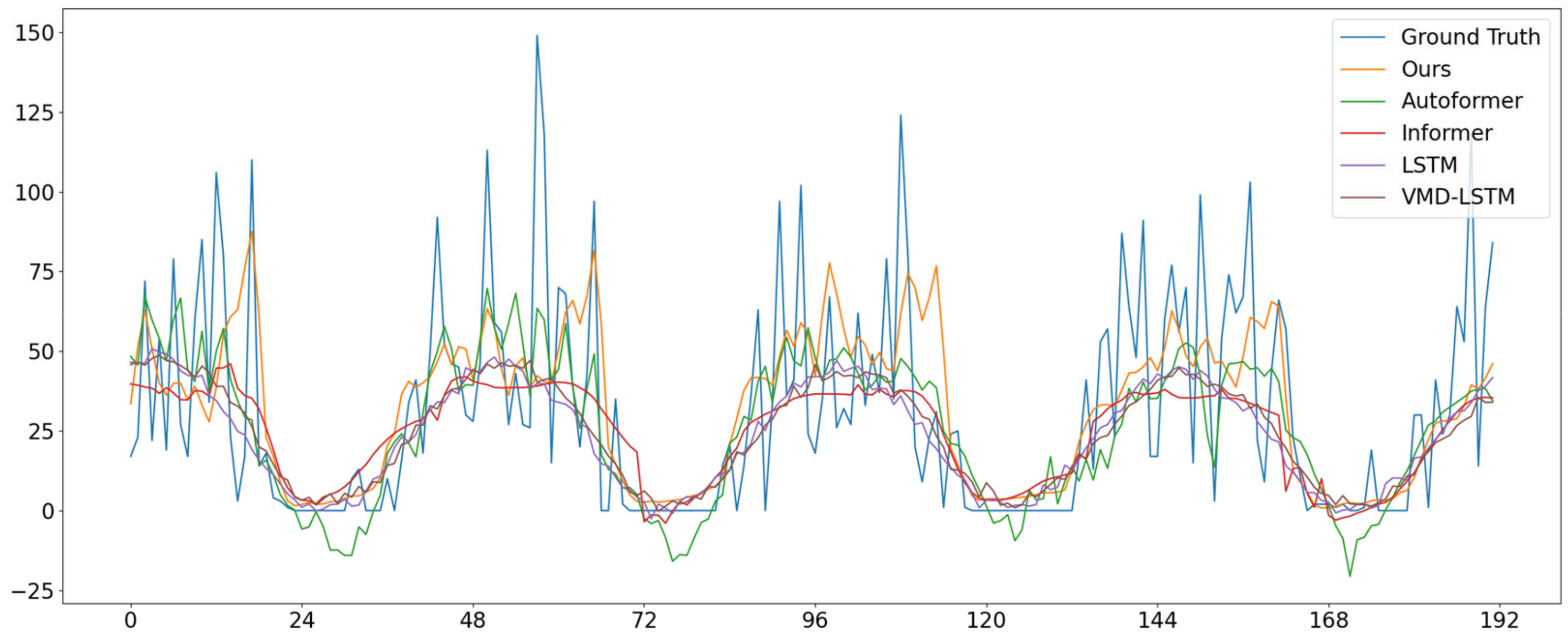
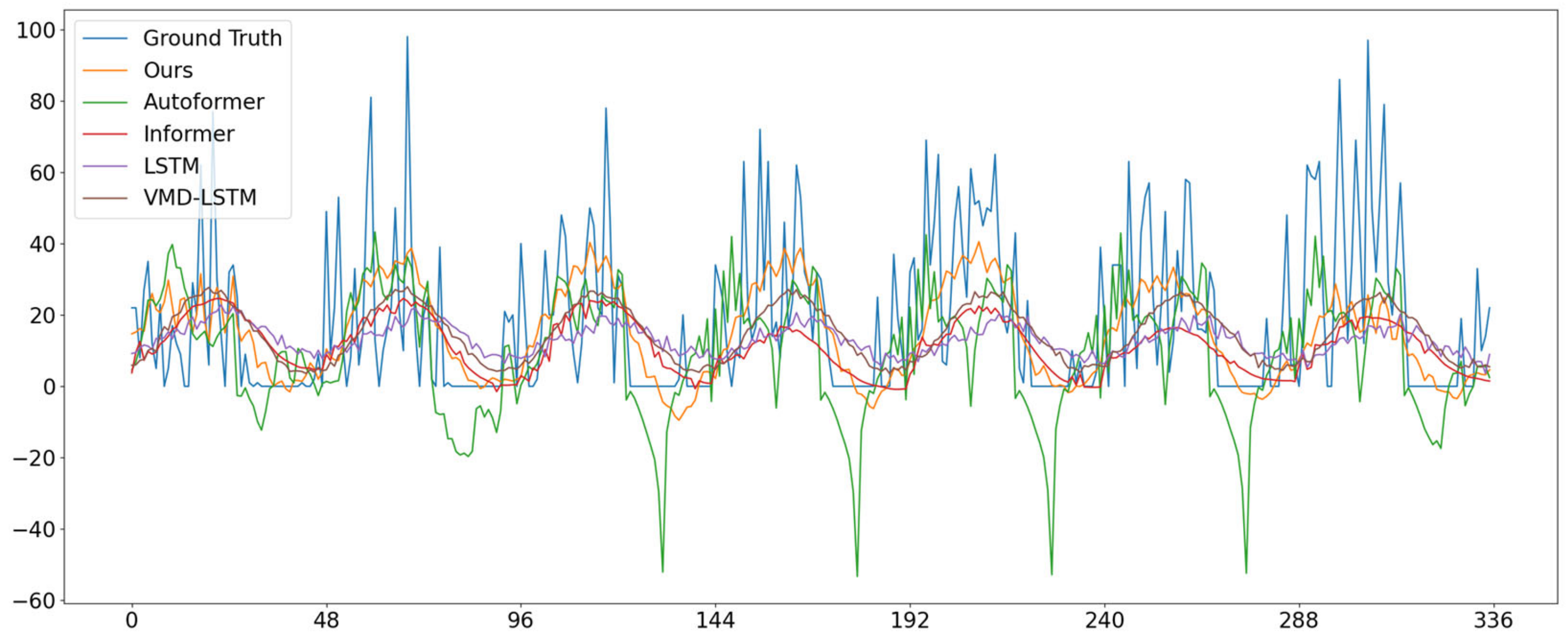
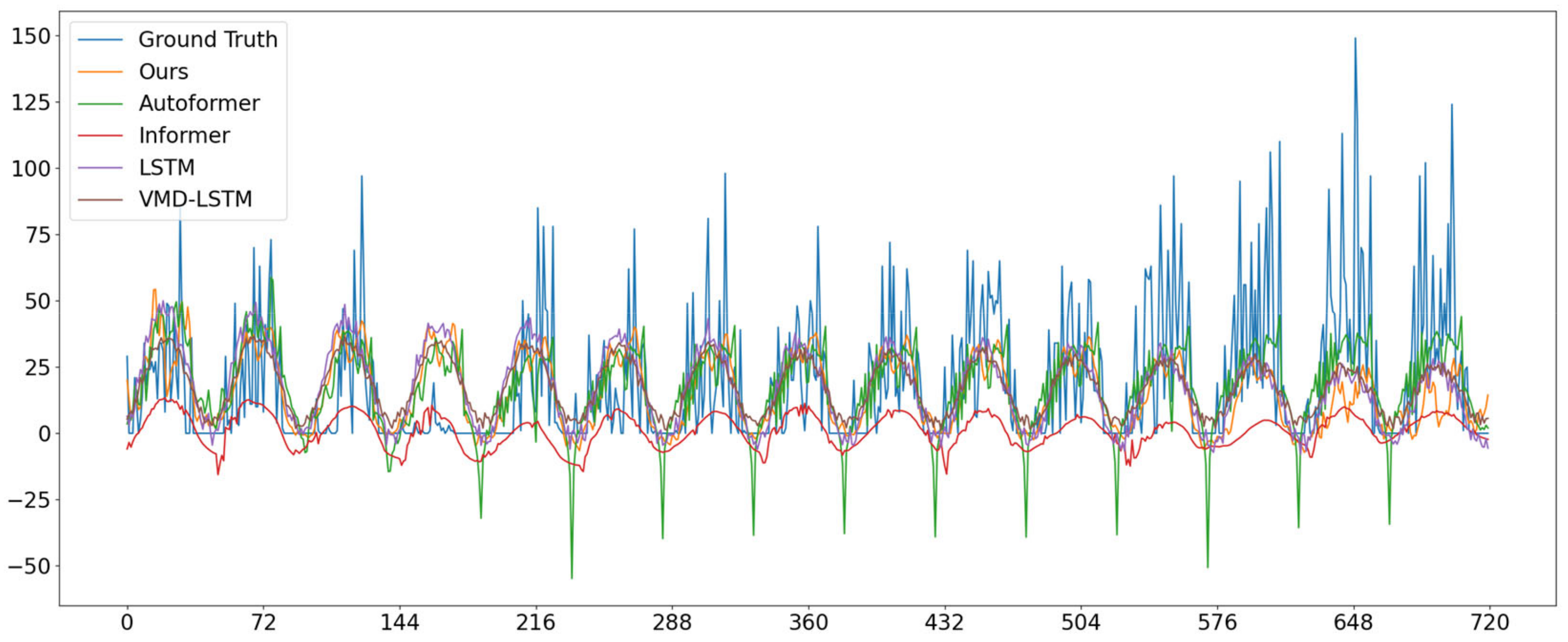
4.2. Compare Experiments

Our experimental platform is shown below: our model is based on python 3.6, pytorch 1.9.0, and the experiments are done on a computer with an Intel i7-7700 CPU and 32 GB of RAM.

Our experiments were conducted with L2 loss function, Adam optimizer, initial learning rate set to 0.0001, batch size set to 32, learning rate changed to 1/2 of the original rate after each run of training data, encoder input length set to 96, decoder input length set to 48+O (96, 192, 336, 720), encoder layer set to 4, and decoder layer set to 2. The number of heads h for multi-head auto-correlation is set to 8. The auto-correlation hyperparameter c is set to 0.3, the training number 20, the number of early stops 3. Each experiment is repeated three times, and the model performance is measured according to the average metrics of the three experiments. The detailed training procedure is shown in Algorithm 1.

Algorithm 1 Training process
1: $\mathbf{Input}: \mathrm{input} \mathrm{past} \mathrm{time} \mathrm{series} \mathrm{X}, \mathrm{input} \mathrm{length} \mathrm{is} \mathrm{I}, \mathrm{prediction} \mathrm{length} \mathrm{is} \mathrm{O}. \mathrm{Data} \mathrm{dimension} \mathrm{is} \mathrm{d}, \mathrm{hidden} \mathrm{state} \mathrm{dimension} \mathrm{is} {\mathrm{d}}_{\mathrm{model}}$$, \mathrm{VMD} \mathrm{decomposition} \mathrm{number} \mathrm{is} \mathrm{K}. (\mathrm{d}=1, {\mathrm{d}}_{\mathrm{model}}$ = 512)
2: ${\mathrm{X}}_{\mathrm{IMF}1},\dots ,{\mathrm{X}}_{\mathrm{IMFK}}=\mathrm{VMD}\left(\mathrm{X}\right)$	$⊳\mathrm{X}\in {ℝ}^{\mathrm{I}\times \mathrm{d}},{\mathrm{X}}_{\mathrm{IMF}1},\dots ,{\mathrm{X}}_{\mathrm{IMFK}}\in {ℝ}^{\mathrm{I}\times \mathrm{d}}$
3: ${\mathrm{X}}_0=\mathrm{Zeros}\left(\left[\mathrm{O},\mathrm{d}\right]\right)$	$⊳{\mathrm{X}}_0\in {ℝ}^{\mathrm{O}\times \mathrm{d}}$
4: ${\mathrm{X}}_{\mathrm{IMF}1}^{\mathrm{DE}},\dots ,{\mathrm{X}}_{\mathrm{IMFK}}^{\mathrm{DE}}=\mathrm{concat}\left({\mathrm{X}}_{\mathrm{IMF}1}^{\frac{\mathrm{I}}{2}:\mathrm{I}},\mathrm{X}0\right),\dots ,\mathrm{concat}\left({\mathrm{X}}_{\mathrm{IMFK}}^{\frac{\mathrm{I}}{2}:\mathrm{I}},\mathrm{X}0\right)$	$⊳{\mathrm{X}}_{\mathrm{IMF}1}^{\mathrm{DE}},\dots ,{\mathrm{X}}_{\mathrm{IMFK}}^{\mathrm{DE}}\in {ℝ}^{\left(\frac{\mathrm{I}}{2}+\mathrm{O}\right)\times \mathrm{d}}$
5: ${\mathrm{S}}_{\mathrm{EN}1},\dots ,{\mathrm{S}}_{\mathrm{ENK}}=\mathrm{Embed}\left({\mathrm{X}}_{\mathrm{IMF}1}\right),\dots ,\mathrm{Embed}\left({\mathrm{X}}_{\mathrm{IMFK}}\right)$	$⊳{\mathrm{S}}_{\mathrm{EN}1},\dots ,{\mathrm{S}}_{\mathrm{ENK}}\in {ℝ}^{\mathrm{I}\times {\mathrm{d}}_{\mathrm{model}}}$
6: ${\mathrm{X}}_{\mathrm{EN}1},\dots ,{\mathrm{X}}_{\mathrm{ENK}}=$$\mathrm{Encoder}\left({\mathrm{S}}_{\mathrm{EN}1}\right),\dots ,\mathrm{Encoder}\left({\mathrm{S}}_{\mathrm{ENK}}\right)$	$⊳{ \mathrm{X}}_{\mathrm{EN}1},\dots ,{\mathrm{X}}_{\mathrm{ENK}}\in {ℝ}^{\mathrm{I}\times {\mathrm{d}}_{\mathrm{model}}}$
7: ${\mathrm{S}}_{\mathrm{DE}1},\dots ,{\mathrm{S}}_{\mathrm{DEK}}=\mathrm{Embed}\left({\mathrm{X}}_{\mathrm{IMF}1}^{\mathrm{DE}}\right),\dots ,\mathrm{Embed}\left({\mathrm{X}}_{\mathrm{IMFK}}^{\mathrm{DE}}\right)$	$⊳{\mathrm{S}}_{\mathrm{DE}1},\dots ,{\mathrm{S}}_{\mathrm{DEK}}\in {ℝ}^{\left(\frac{\mathrm{I}}{2}+\mathrm{O}\right)\times {\mathrm{d}}_{\mathrm{model}}}$
8: ${\mathrm{X}}_{\mathrm{DE}1},\dots ,{\mathrm{X}}_{\mathrm{DEK}}=\mathrm{Decoder}\left({\mathrm{S}}_{\mathrm{DE}1},{\mathrm{X}}_{\mathrm{EN}1}\right),\dots ,\mathrm{Decoder}\left({\mathrm{S}}_{\mathrm{DEK}},{\mathrm{X}}_{\mathrm{ENK}}\right)$
9: ${\mathrm{X}}_{\mathrm{EN}}={\mathrm{X}}_{\mathrm{EN}1}+{\mathrm{X}}_{\mathrm{EN}2}+\dots +{\mathrm{X}}_{\mathrm{ENK}}$	$⊳{\mathrm{X}}_{\mathrm{EN}}\in {ℝ}^{\mathrm{I}\times {\mathrm{d}}_{\mathrm{model}}}$
10: ${\mathrm{X}}_{\mathrm{DE}}={\mathrm{X}}_{\mathrm{DE}1}+{\mathrm{X}}_{\mathrm{DE}2}+\dots +{\mathrm{X}}_{\mathrm{DEK}}$	$⊳{\mathrm{X}}_{\mathrm{DE}1},\dots ,{\mathrm{X}}_{\mathrm{DEK}}\in {ℝ}^{\left(\frac{\mathrm{I}}{2}+\mathrm{O}\right)\times {\mathrm{d}}_{\mathrm{model}}},{\mathrm{X}}_{\mathrm{DE}}\in {ℝ}^{\left(\frac{\mathrm{I}}{2}+\mathrm{O}\right)\times {\mathrm{d}}_{\mathrm{model}}}$
11: ${\mathrm{X}}_{\mathrm{EN}}^{\mathrm{last}}=\mathrm{Encoder}\left({\mathrm{X}}_{\mathrm{EN}}\right)$	$⊳{\mathrm{X}}_{\mathrm{EN}}^{\mathrm{last}}\in {ℝ}^{\mathrm{I}\times {\mathrm{d}}_{\mathrm{model}}}$
12: ${\mathrm{X}}_{\mathrm{DE}}^{\mathrm{last}}=\mathrm{Decoder}\left({\mathrm{X}}_{\mathrm{DE}},{\mathrm{X}}_{\mathrm{EN}}^{\mathrm{last}}\right)$	$⊳{\mathrm{X}}_{\mathrm{DE}}^{\mathrm{last}}\in {ℝ}^{\left(\frac{\mathrm{I}}{2}+\mathrm{O}\right)\times {\mathrm{d}}_{\mathrm{model}}}$
13: $Return{ \mathrm{X}}_{\mathrm{pred}}=\mathrm{feedforward}\left({\mathrm{X}}_{\mathrm{DE}}^{\mathrm{last}}\right)$	$⊳{\mathrm{X}}_{\mathrm{pred}}\in {ℝ}^{\left(\frac{\mathrm{I}}{2}+\mathrm{O}\right)\times \mathrm{d}}$
14: $\mathrm{loss}=\mathrm{nn}.\mathrm{MSELoss}\left({ \mathrm{X}}_{\mathrm{pred}}\left[-\mathrm{O}:\right],\mathrm{X}\right)$
15: $\mathrm{model}.\mathrm{backward}\left( \right)$
16: Repeat above all
17: Until the stopping criteria are met
18: Ending the program

We compare autoformer, informer, lstm, and vmd-lstm as baseline comparison models with our model to further demonstrate the superiority of our model. The dimension of the hidden layer of the LSTM is set to 256 and the number of network layers is set to 3. The parameter settings in the VMD-LSTM remain the same as those of the LSTM. The parameters of autoformer and informer are set according to the default configuration of the author.

We present the experimental results of our model and other baseline models in Figure 7. The experimental results are obtained from the data in the test set. The prediction lengths are 96, 192, 336, and 720, which are reflecting the meaning of long-term traffic flow prediction. The prediction lengths from short to long better reflect the real performance of a model. When the forecast length is 96, the MSE of our model decreases by 3.6% (0.307 → 0.296) and the MAE of our model decreases by 4.4% (0.390 → 0.373) compared with other models, and some of the forecast results are shown in Figure 8. When the prediction length is 192, the MSE of our model decreases by 0.6% (0.340 → 0.338) and the MAE of our model decreases by 0.8% (0.391 → 0.388) compared with the other models, and some of the prediction results are shown in Figure 9. When the prediction length is 336, the MSE of our model decreases by 4.6% (0.371 → 0.354) and the MAE of our model decreases by 5.8% (0.417 → 0.393) compared with the other models, and some of the prediction results are shown in Figure 10. When the prediction length is 720, the MSE of our model is 7.1% (0.390 → 0.362) lower than the other models, and the MAE of our model is 8.4% (0.431 → 0.395) lower than the other models, and some of the prediction results are shown in Figure 11. Compared with other baseline models, the prediction of our model maintains a certain advantage from a prediction length of 96 to a prediction length of 720, showing the accuracy and stability of our model’s prediction.

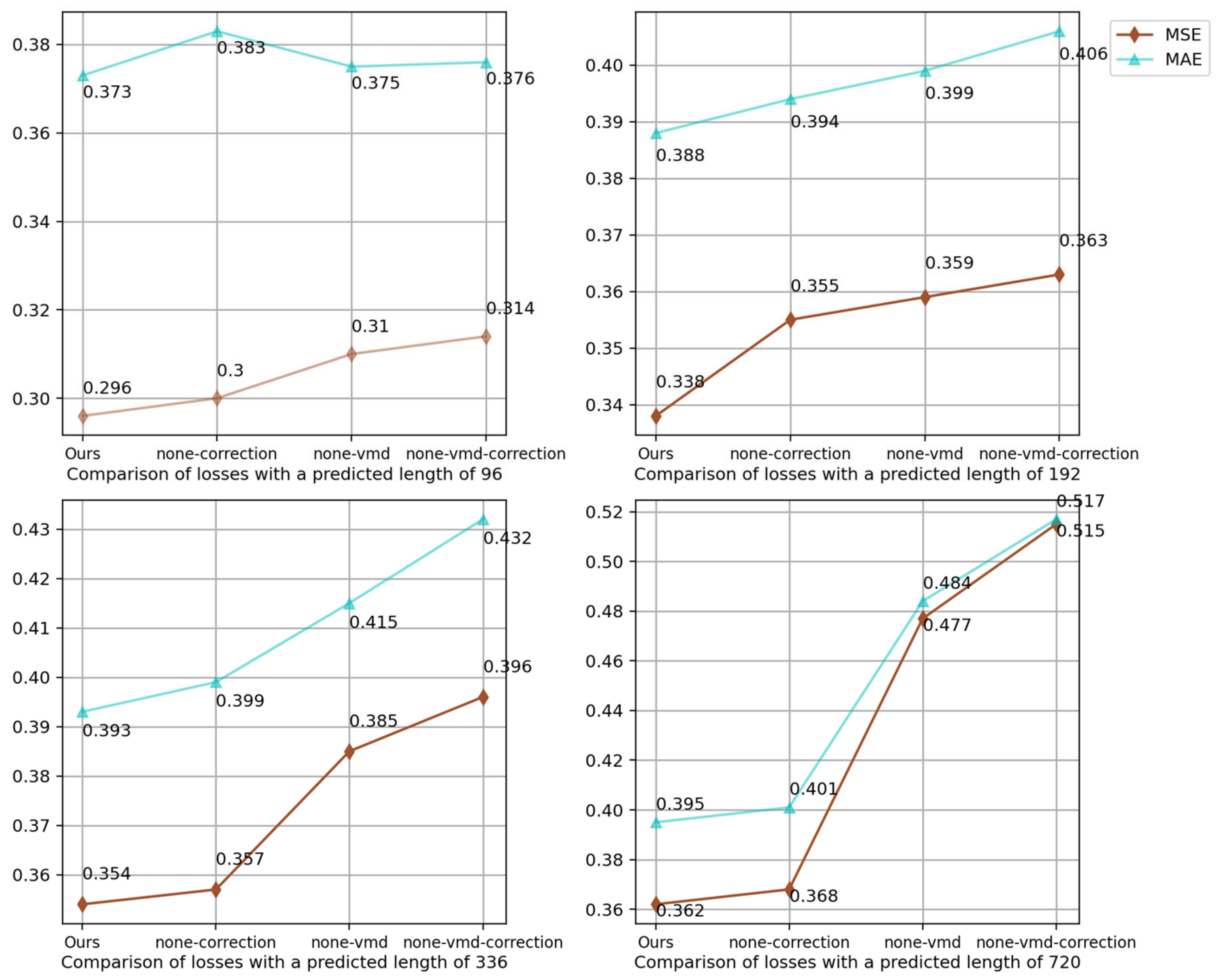
4.3. Ablation Experiments

In this section, we test the role played by VMD and the correction module in the prediction effect of the model. The specific experimental results are shown in Figure 12. The experimental results were obtained from the test set. The model with VMD and the correction module applied achieves the best prediction performance.

The model with the correction module removed is compared with the model with the VMD and correction module removed to verify the key role played by VMD in the prediction. In experiments with prediction lengths of 96, 192, 336, and 720, MSE decreases by 4.5% (0.314 → 0.300), 2.2% (0.363 → 0.355), 9.8% (0.396 → 0.357), and 28.5% (0.515 → 0.368), respectively. The role played by VMD in longer predictions is more obvious; the model with VMD removed is compared with the model with VMD and correction module removed to verify the usefulness of the correction module. In the experiments with prediction lengths of 96, 192, 336, and 720, the MSE decreased by 1.3% (0.314 → 0.310), 1.1% (0.363 → 0.359), 2.8% (0.396 → 0.385), and 7.3% (0.515 → 0.477), respectively. The application of the correction module has resulted in a slight improvement in the performance of the model. From the Figure 12, it can be seen that the longer the prediction length, the more obvious the effect of VMD and correction module on the prediction accuracy, especially the VMD is very effective for long-term prediction.

5. Conclusions and Future Research

To fully utilize the traffic flow data, we propose a method of VMD to decompose the data into different frequency components. We then construct encoders and decoders using the auto-correlation mechanism for each frequency component. The encoder and decoder are used to extract features from the corresponding frequency component, and a correction module is introduced to improve the residual structure of the encoder and decoder. Through comparative experimental demonstration, our model achieves the best prediction results for prediction lengths ranging from 96 to 720. In the ablation experiments, we verify the key role played by VMD and the correction module in improving the overall performance of the model. As the prediction length increases, the improvement in prediction effect due to VMD decomposition becomes more pronounced. Additionally, the correction module enhances the robustness of the model. Our model is able to fully extract the internal features of the data to make a more comprehensive prediction. Our model has high prediction accuracy and stable prediction performance, especially for long-term prediction. It enriches the research on long-term traffic flow prediction.

Traffic flow prediction is a complex task that is influenced by various factors beyond the past traffic flow data. Factors such as weather conditions, holidays, and other contextual variables can significantly impact traffic flow changes. Furthermore, it has been observed that there exist hidden connections between traffic flows in different locations. Therefore, investigating the influence of these external factors on traffic flow prediction, including their hidden features, holds great potential for improving the accuracy of future predictions.

References

1. An, J.; Fu, L.; Hu, M.; Chen, W.; Zhang, J. A novel fuzzy-based convolutional neural network method to traffic flow prediction with uncertain traffic accident information. IEEE Access 2019, 7, 20708–20722. [Google Scholar] [CrossRef]
2. Liu, Y.; Wang, X.; Hou, W.; Liu, H.; Wang, J. A novel hybrid model combining a fuzzy inference system and a deep learning method for short-term traffic flow prediction. Knowl.-Based Syst. 2022, 255, 109760. [Google Scholar] [CrossRef]
3. Kumar, S.V.; Vanajakshi, L. Short-term traffic flow prediction using seasonal ARIMA model with limited input data. Eur. Transp. Res. Rev. 2015, 7, 21. [Google Scholar] [CrossRef] [Green Version]
4. Chen, C.; Hu, J.; Meng, Q.; Zhang, Y. Short-time traffic flow prediction with ARIMA-GARCH model. In Proceedings of the 2011 4nd IEEE Conference on Intelligent Vehicles Symposium, Baden-Baden, Germany, 5–9 June 2011; pp. 607–612. [Google Scholar]
5. Wei, Y.; Liu, H. Convolutional Long-Short Term Memory Network with Multi-Head Attention Mechanism for Traffic Flow Prediction. Sensors 2022, 22, 7994. [Google Scholar] [CrossRef] [PubMed]
6. Zhang, L.; Lin, W. Calibration-free Traffic Signal Control Method Using Machine Learning Approaches. In Proceedings of the 2022 International Conference on Electrical, Computer and Energy Technologies (ICECET), Prague, Czech Republic, 20–22 July 2022; pp. 1–6. [Google Scholar]
7. Gu, J.; Jia, Z.; Cai, T.; Song, X.; Mahmood, A. Dynamic correlation adjacency-matrix-based graph neural networks for traffic flow prediction. Sensors 2023, 23, 2897. [Google Scholar] [CrossRef]
8. Braz, F.J.; Ferreira, J.; Gonçalves, F.; Weege, K.; Almeida, J.; Baldo, F.; Goncalves, P. Road traffic forecast based on meteorological information through deep learning methods. Sensors 2022, 22, 4485. [Google Scholar] [CrossRef]
9. Tong, M.; Xue, H. Highway traffic volume forecasting based on seasonal ARIMA model. J. Highw. Transp. Res. Dev. Engl. Ed. 2008, 3, 109–112. [Google Scholar] [CrossRef]
10. Bai, S.; Kolter, J.Z.; Koltun, V. An empirical evaluation of generic convolutional and recurrent networks for sequence modeling. arXiv 2018, arXiv:1803.01271. [Google Scholar]
11. Hochreiter, S.; Schmidhuber, J. Long short-term memory. Neural Comput. 1997, 9, 1735–1780. [Google Scholar] [CrossRef]
12. Cho, K.; Van Merriënboer, B.; Bahdanau, D.; Bengio, Y. On the properties of neural machine translation: Encoder-decoder approaches. arXiv 2014, arXiv:1409.1259. [Google Scholar]
13. Vaswani, A.; Shazeer, N.; Parmar, N.; Parmar, N.; Uszkoreit, J.; Jones, L.; Gomez, A.N.; Kaiser, L.; Polosukhin, I. Attention is all you need. In Proceedings of the 2017 Conference on Advances in Neural Information Processing Systems, Long Beach, CA, USA, 4–9 December 2017; Volume 30, pp. 5998–6008. [Google Scholar]
14. Huang, N.E.; Shen, Z.; Long, S.R.; Wu, M.C.; Shih, H.H.; Zheng, Q.; Yen, N.C.; Tung, C.C.; Liu, H.H. The empirical mode decomposition and the Hilbert spectrum for nonlinear and non-stationary time series analysis. Proc. R. Soc. Lond. Ser. A 1998, 454, 903–995. [Google Scholar] [CrossRef]
15. Dragomiretskiy, K.; Zosso, D. Variational mode decomposition. IEEE Trans. Signal Process. 2013, 62, 531–544. [Google Scholar] [CrossRef]
16. Cong, Y.; Wang, J.; Li, X. Traffic flow forecasting by a least squares support vector machine with a fruit fly optimization algorithm. Procedia Eng. 2016, 137, 59–68. [Google Scholar] [CrossRef] [Green Version]
17. Zhang, L.; Alharbe, N.R.; Luo, G.; Yao, Z.; Li, Y. A hybrid forecasting framework based on support vector regression with a modified genetic algorithm and a random forest for traffic flow prediction. Tsinghua Sci. Technol. 2018, 23, 479–492. [Google Scholar] [CrossRef]
18. Sun, B.; Cheng, W.; Goswami, P.; Bai, G. Short-term traffic forecasting using self-adjusting k-nearest neighbours. IET Intell. Transp. Syst. 2018, 12, 41–48. [Google Scholar] [CrossRef] [Green Version]
19. Zhang, N.; Zhang, Y.; Lu, H. Short-term freeway traffic flow prediction combining seasonal autoregressive integrated moving average and support vector machines. In Proceedings of the 90th Board Annual Conference on Transportation Research, Washington, DC, USA, 23–27 January 2011; pp. 1–16. [Google Scholar]
20. Cai, L.; Yu, Y.; Zhang, S.; Song, Y.; Xiong, Z.; Zhou, T. A sample-rebalanced outlier-rejected $ k $-nearest neighbor regression model for short-term traffic flow forecasting. IEEE Access 2020, 8, 22686–22696. [Google Scholar] [CrossRef]
21. Zhao, W.; Gao, Y.; Ji, T.; Wan, X.; Ye, F.; Bai, G. Deep temporal convolutional networks for short-term traffic flow forecasting. IEEE Access 2019, 7, 114496–114507. [Google Scholar] [CrossRef]
22. Yang, B.; Sun, S.; Li, J.; Lin, X.; Tian, Y. Traffic flow prediction using LSTM with feature enhancement. Neurocomputing 2019, 332, 320–327. [Google Scholar] [CrossRef]
23. Ali, A.; Zhu, Y.; Zakarya, M. A data aggregation based approach to exploit dynamic spatio-temporal correlations for citywide crowd flows prediction in fog computing. Multimed. Tools. Appl. 2021, 80, 31401–31433. [Google Scholar] [CrossRef]
24. Luo, X.; Li, D.; Yang, Y.; Zhang, S. Spatiotemporal traffic flow prediction with KNN and LSTM. J. Adv. Transp. 2019, 2019, 4145353. [Google Scholar] [CrossRef] [Green Version]
25. Zhao, Z.; Chen, W.; Wu, X.; Chen, P.C.Y.; Liu, J. LSTM network: A deep learning approach for short-term traffic forecast. IET Intell. Transp. Syst. 2017, 11, 68–75. [Google Scholar] [CrossRef] [Green Version]
26. Liu, Y.; Zheng, H.; Feng, X.; Chen, Z. Short-term traffic flow prediction with Conv-LSTM. In Proceedings of the 2017 9th International Conference on Wireless Communications and Signal Processing (WCSP), Nanjing, China, 11–13 October 2017; pp. 1–6. [Google Scholar]
27. Fu, R.; Zhang, Z.; Li, L. Using LSTM and GRU neural network methods for traffic flow prediction. In Proceedings of the 2016 31st Youth Academic Annual Conference of Chinese Association of Automation (YAC), Wuhan, China, 11–13 November 2016; pp. 324–328. [Google Scholar]
28. Zhaowei, Q.; Haitao, L.; Zhihui, L.; Tao, Z. Short-term traffic flow forecasting method with MB-LSTM hybrid network. IEEE Trans. Intell. Transp. Syst. 2020, 23, 225–235. [Google Scholar] [CrossRef]
29. Zhou, H.; Zhang, S.; Peng, J.; Zhang, S.; Li, J.; Xiong, H.; Zhang, W. Informer: Beyond effificient transformer for long sequence time-series forecasting. Proc. AAAI Conf. Artif. Intell. 2021, 35, 11106–11115. [Google Scholar] [CrossRef]
30. Wu, H.; Xu, J.; Wang, J.; Long, M. Autoformer: Decomposition transformers with auto-correlation for long-term series forecasting. Adv. Neural Inf. Process. Syst. 2021, 34, 22419–22430. [Google Scholar]
31. Zhou, T.; Ma, Z.; Wen, Q.; Wang, X.; Sun, L.; Jin, R. Fedformer: Frequency enhanced decomposed transformer for long-term series forecasting. arXiv 2022, arXiv:2201.12740. [Google Scholar]
32. Hao, W.; Sun, X.; Wang, C.; Chen, H.; Huang, L. A hybrid EMD-LSTM model for non-stationary wave prediction in offshore China. Ocean Eng. 2022, 246, 110566. [Google Scholar] [CrossRef]
33. Li, Y.; Chai, S.; Ma, Z.; Wang, G. A hybrid deep learning framework for long-term traffic flow prediction. IEEE Access 2021, 9, 11264–11271. [Google Scholar] [CrossRef]
34. Huang, Y.; Deng, Y. A new crude oil price forecasting model based on variational mode decomposition. Knowl.-Based Syst 2021, 213, 106669. [Google Scholar] [CrossRef]
35. Niu, H.; Xu, K.; Wang, W. A hybrid stock price index forecasting model based on variational mode decomposition and LSTM network. Appl. Intell. 2020, 50, 4296–4309. [Google Scholar] [CrossRef]
36. Hu, H.; Wang, L.; Tao, R. Wind speed forecasting based on variational mode decomposition and improved echo state network. Renew. Energ. 2021, 164, 729–751. [Google Scholar] [CrossRef]
37. Zhang, Z.; Hong, W.C. Application of variational mode decomposition and chaotic grey wolf optimizer with support vector regression for forecasting electric loads. Knowl.-Based Syst. 2021, 228, 107297. [Google Scholar] [CrossRef]
38. Bing, Q.; Shen, F.; Chen, X.; Zhang, W.; Hu, Y.; Qu, D. A hybrid short-term traffic flow multistep prediction method based on variational mode decomposition and long short-term memory model. Discrete Dyn. Nat. Soc. 2021, 2021, 4097149. [Google Scholar] [CrossRef]
39. Liu, H.; Zhang, X.; Yang, Y.; Li, Y.; Yu, C. Hourly traffic flow forecasting using a new hybrid modelling method. J. Cent. South Univ. 2022, 29, 1389–1402. [Google Scholar] [CrossRef]
40. Tang, J.; Chien, Y.R. Research on Wind Power Short-Term Forecasting Method Based on Temporal Convolutional Neural Network and Variational Modal Decomposition. Sensors 2022, 22, 7414. [Google Scholar] [CrossRef]
41. Cai, C.; Li, Y.; Su, Z.; Zhu, T.; He, Y. Short-Term Electrical Load Forecasting Based on VMD and GRU-TCN Hybrid Network. Appl. Sci. 2022, 12, 6647. [Google Scholar] [CrossRef]
Figure 1. VMD algorithm flow chart.
Applsci 13 07139 g001
Figure 2. Auto-correlation mechanism (left) and time delay aggregation (right).
Applsci 13 07139 g002
Figure 3. Schematic diagram of the correction module (blue dashed part is the correction module).
Applsci 13 07139 g003
Figure 4. Structure of VMD–auto-correlation model.
Applsci 13 07139 g004
Figure 5. Encoder and decoder structure.
Applsci 13 07139 g005
Figure 6. Data plot (original data, normalized data, and decomposed imf components).
Applsci 13 07139 g006
Figure 7. Comparison of prediction results of different models.
Applsci 13 07139 g007
Figure 8. Partial prediction results for a prediction length of 96.
Applsci 13 07139 g008
Figure 9. Partial prediction results for a prediction length of 192.
Applsci 13 07139 g009
Figure 10. Partial prediction results for a prediction length of 336.
Applsci 13 07139 g010
Figure 11. Partial prediction results for a prediction length of 720.
Applsci 13 07139 g011
Figure 12. Comparison of the results of ablation experiments.
Applsci 13 07139 g012