Image-Based Crack Detection Using Total Variation Strain DVC Regularization

Abstract

Introduction: Accurately detecting cracks is crucial for assessing the health of materials. Manual detection methods are time-consuming, leading to the development of automatic detection techniques based on image processing and machine learning. These methods utilize morphological image processing and material deformation analysis through Digital Image or Volume Correlation techniques (DIC/DVC) to identify cracks. The strain field derived from DIC/DVC tends to be noisy. Traditional denoising methods sacrifice spatial resolution, limiting their effectiveness in capturing abrupt structural deformations such as fractures. Method: In this study, a novel DVC regularization method is proposed to obtain a sharper and less noisy strain field. The method minimizes the total variation of spatial strain field components based on the assumption of approximate strain constancy within material phases. Results: The proposed methodology is validated using simulated data and actual 4D $\mathsf{\mu }$-CT experimental data. Compared to classical denoising methods, the proposed DVC regularization method provides a more reliable crack detection with fewer false positives. Conclusions: These results highlight the possibility of estimating a low-noise strain field without relying on the spatial smoothness assumption, thereby improving accuracy and reliability in crack detection.

1. Introduction

Image-based crack detection is a significant subfield of image analysis that has garnered considerable attention in recent years [1]. Typically, cracks in materials occur at the microscopic level, and their early detection can prevent further damage. When identifying cracks through images, it is crucial to employ methods that effectively preserve the spatial resolution of the analyzed problem, ensuring, at the same time, minimal influence from image noise. However, it is important to note that crack-detection methods based on Digital Volume Correlation (DVC) techniques tend to be insufficient in addressing this aspect. This limitation often presents users with a trade-off, forcing them to choose between a solution that offers higher spatial resolution but lower signal-to-noise ratio (SNR), or vice versa.

Visual inspection remains a common method for detecting cracks, yet it is prone to limitations such as subjectivity and reliance on the expertise of the specialist. Moreover, it is time-consuming and exhibits low reproducibility, especially in the case of 3D analysis [2]. As a result, there is a growing need to develop alternative crack-detection methods that are more accurate, efficient, and consistent.

Over the years, image-based methods for crack detection have been developed to address the limitations of manual annotation. These methods offer several advantages, including automation, efficiency, and improved reliability. Image-based crack-detection methods can be broadly classified into two categories: direct methods and indirect methods. Direct methods are based on variations in gray scale or color pixel intensities [3], as shown in Figure 1a. Indirect methods rely on the results of Digital Image and Volume Correlation techniques (DIC/DVC), as shown in Figure 1b. Direct methods typically involve a pre-processing step [1,4,5], such as smoothing, filtering, or contrast enhancement, followed by a detection step, which may use morphological, statistical [6,7] (e.g., Gabor filter bank (GFB), Grey Level Co-occurrence Matrix (GLCM), Local Binary Matrix Feature Extraction (LBFE)), or machine learning methods [1,8,9]. Pixel-intensity-based crack detectors depend on the lighting conditions and require a homogeneous appearance of the uncracked areas [10]; indeed one of the main limitations of the image-based techniques is that the surface noise might be considered a crack [11]. In DIC, to mitigate this problem, often the cracks are painted in white, but this is not possible for 3D problems. Moreover, pixel-intensity-based methods can achieve a precision more than one order of magnitude below the pixel’s size [10] and they are unable to detect the direction of the propagation of cracks properly [11]. To overcome the limitations of direct image-based crack measurements, there has been an increasing use of indirect techniques based on DIC and DVC [10,12]. However, the main advantage of direct over indirect methods is that they do not require a pre-deformed acquisition (reference frame) and an acquisition in the deformed configuration.

The proposed crack-detection method belongs to the category of indirect methods, which rely on information provided by the displacement and/or strain field. In contrast to direct methods, indirect methods identify cracks by detecting discontinuities in the displacement field, which correspond to peaks in the strain field [10,13]. The displacement and strain fields used in this study are computed from images using digital image and volume correlation techniques [14]. From a mechanical perspective, the use of DVC to compute the strain field can provide valuable insights into the deformation behavior of the material and its response to external loading conditions.

The accurate computation and analysis of the strain field is critical in indirect image-based crack-detection methods: modeling a sharp strain field that can describe abrupt deformations is challenging. While some methods can compute sharp displacement fields with discontinuities [15,16], the sharpness of the resulting strain field may not be preserved. This is due to the spatial mathematical differentiation of the estimated displacement field to compute the strain field, which amplifies small, high-frequency variations, noise, and errors in the displacement field. To mitigate this issue, various solutions have been proposed, including post-processing techniques such as smoothing the displacement field before differentiation. Common approaches, summarized in Table 1, include using average, median, and Gaussian mean filters [17,18,19,20]. Gaussian filters are applied by replacing each pixel’s value with the average of the neighboring pixels, weighted using a Gaussian kernel. However, Gaussian filters are not suitable for interface-related issues as they may inadvertently average the pixel intensities from both sides of the interface. Average filters substitute each value in the region of interest with the average (or weighted average) of the values within the neighborhood specified by the filter mask. Average filters substitute each value in the region of interest with the average (or weighted average) of the values within the neighborhood specified by the filter mask. This approach results in information loss at the edges and borders of the filtered data. Therefore, this method is also not suitable for interface-related issues. Median filters are effective in smoothing strain fields while preserving edges. This filtering technique involves replacing each pixel’s value with the median value of its neighborhood. The size of the selected window dimension affects the locality of the solution [10].

Another alternative is to compute the strain from the noisy displacement field first and then apply a filter to the strain field [17,21,22]. These techniques are applied in many DIC/DVC open-source and commercial software, such as those offered by [18,19,22].

Table 1. An overview of methods employed for reducing noise in strain field.

Technique	Parameters	Disadvantages
Gaussian filters [20]	Window size, standard deviation	Not suitable for interface-related issue
Median filters [10]	Window size	Challenges related to identifying narrow gaps between cracks
Average filter [17]	Window size, weight	Loss of information at the edges and borders
PLS [23,24,25]	Window size	Trade-off between noise reduction and window size
Geers’ method [22,26]	Number of neighboring points	Trade-off between noise reduction and locality of the solution

Table 1. An overview of methods employed for reducing noise in strain field.

Technique	Parameters	Disadvantages
Gaussian filters [20]	Window size, standard deviation	Not suitable for interface-related issue
Median filters [10]	Window size	Challenges related to identifying narrow gaps between cracks
Average filter [17]	Window size, weight	Loss of information at the edges and borders
PLS [23,24,25]	Window size	Trade-off between noise reduction and window size
Geers’ method [22,26]	Number of neighboring points	Trade-off between noise reduction and locality of the solution

In some cases, alternatives to filtering methods have been employed such as planar approximation (2D) [23], point-wise least-squares (PLS) algorithm, both in 2D and 3D [24,25] and Geers’ method in 3D [26]. These methods are implemented in MatchID [23], Ncorr [27], and SPAM [22]. The PLS method involves the definition of a window around the voxels where the strain needs to be computed, if the window is small enough the strain can be approximated as linear. Geers’ method computes strains from the displacements in a discrete set of points in the neighborhood. The local differences in the displacements have been expanded in a Taylor series, which was truncated after the second-quadratic term [26]. Both these methods reduce the locality of the solution. A trade-off between noise and spatial resolution exists in the computation of the strain field, which leads to a reduction in the resolution despite having a sharp displacement field. Fractures are usually associated with localized discontinuities in the displacement field and peaks in the strain [10].

To overcome the challenge of obtaining a sharp and low noise strain field, we propose a novel DVC regularization method. Our approach is based on minimizing the spatial total variation of the strain field (TV-reg). By minimizing the total variation, our method promotes a piecewise constant strain profile that allows for discontinuities in the strain field. The constraint of piecewise constant strain field inside the distinct structures that compose the material leads to a strain field with a higher signal-to-noise ratio.

2. Method

Image registration is the basis of DVC, and it consists of aligning features in the moving image to the reference image by using a displacement field. The estimation of the D-dimensional displacement field $\mathbf{u}:\mathrm{\Omega }\to {\mathbf{R}}^D$, that maps the moving image $I_m:\mathrm{\Omega }\to \mathbf{R}$ to the reference image $I_f:\mathrm{\Omega }\to \mathbf{R}$, requires the minimization of a cost function

$$\begin{array}{c}\hfill \widehat{\mathbf{u}}=arg\underset{\mathbf{u}}{min}(C_s(\mathbf{u};I_f,I_m)+\lambda C_R\left(\mathbf{u}\right))\end{array}$$

(1)

where $\mathrm{\Omega }$ is the image domain, $C_S$ is the image similarity metric, $C_R$ is the regularization term, and $\lambda >0$ is the weight of the regularization in the cost function. The image similarity metric measures how well the moving image matches the reference image. The metric should be chosen based on the images to be registered and the kind of misalignment, there is no clear rule for which metric should be chosen.

The regularization term ($C_R$) constitutes the second component of the cost function and is essential due to the ill-posed nature of image registration. The available information from the image data, represented by gray intensity scalar values, is insufficient to guarantee a unique solution for the displacement field, which consists of a vector with three unknowns. To address this, constraints must be imposed on the displacement field to establish a well-posed problem. The introduction of constraints, known as regularization, restricts the degrees of freedom in the solution, ensuring a mechanically admissible DVC solution. The similarity metric together with the regularization term constitutes the objective function to be optimized over the search space that comprises the parameters of the transformation. The transformation serves as the spatial mapping of points from the moving image to the fixed image. Various types of transformations are available for this purpose, which are discussed in more detail in Section 2.3 of this paper. After obtaining the optimal values for the transformation parameters, the interpolator is employed to determine the intensities of the moving volume at positions where the parameters are not defined.

2.1. Proposed Method: Total Variation Strain Field Regularization (TV-Reg)

The proposed methodology is based on DVC technique with the incorporation of a regularization step. The innovation lies in the introduction of a regularization term defined by the Total Variation of the strain field. The objective is to minimize the TV of the strain field, which enforces a piecewise constant strain profile while permitting discontinuities (jumps) in the strain field. The cost function to be optimized comprises an image-based similarity metric and a strain field-based TV metric. The optimization of this function requires balancing the trade-off between data fit, represented by the similarity metric, and deformation discontinuity.

DVC has been performed by using a B-spline function as model to describe the deformation. In this way, a parametrization of the displacement field was possible and that allows the dimensionality of the registration optimization problem to be reduced.

2.2. Spatial Total Variation Strain Field Regularization

The TV strain field regularization is defined as the $l_1-norm$ of the strain field gradients

$$C_R^{TV}=\sum _{m,n=1}^D{\parallel \Delta {ϵ}_{mn}\left(\mathbf{u}\left(\mathbf{x}\right)\right)\parallel }_1=\sum _{x\in \mathrm{\Omega }}\sqrt{\sum _{j,m,n=1}^D{\left({\Delta }_j{ϵ}_{mn}\left(\mathbf{u}\left(\mathbf{x}\right)\right)\right)}^2}$$

(2)

where $\Delta$ is the finite differences operator, $ϵ$ is the 3D Lagrangian strain computed in each point x of the image domain $\mathrm{\Omega }$ (see Appendix A), and D is the spatial dimension. The term $C_R^{TV}$ promotes non-smooth piecewise constant strain field. The regularization term must be weighed properly in order to penalize the small variations of the strain field (due to noise) and to preserve important details of the images such as discontinuities. The relative weight is introduced by the multiplicative factor ${\lambda }_{TV}$. The choice of the optimal ${\lambda }_{TV}$ depends on the type of motion and the image noise level. This dependency has been discussed in Section 5.

The final cost function to be minimized, in addition to the total variation regularization term, contains the similarity metric. In this research, the selected similarity metric is the sum of squared differences (SSD). The SSD metric is based on the voxel intensity differences between two images, and it aims to minimize the average squared intensity differences between them. Mathematically, the cost function can be defined as:

$$\underset{\begin{array}{c}{C}_S\end{array}}{\underbrace{\sum _{x\in \mathrm{\Omega }}{(I_f\left(\mathbf{x}\right)-I_m(\mathbf{x}+\mathbf{u}\left(\mathbf{x}\right)))}^2}}+{\lambda }_{TV}\underset{\begin{array}{c}{C}_R^{TV}\end{array}}{\underbrace{\sum _{x\in \mathrm{\Omega }}\sqrt{\sum _{j,m,n=1}^D{\left({\Delta }_j{ϵ}_{mn}\left(\mathbf{u}\left(\mathbf{x}\right)\right)\right)}^2}}}$$

(3)

2.3. Parametric Transformations

Different models to describe the deformation have been used in literature. It is possible to make a macro distinction between “non-parametric” and “parametric” models. Among “non-parametric” models may be cited: diffeomorphic image registration methods [28], image registration using Fourier transformation [24], and image registration based on physical models [29]. Among “parametric” models the B-spline model [30,31,32] and the thin plate splines model [33,34] are the most commonly used.

The parametrization of the displacement field allows the dimensionality of the optimization problem to be reduced and the size of the parameter search space to be constrained to allow realistic displacement fields. The parametrization is imposed on a mesh $n_x\times n_y\times n_z$ of control points ${\Phi }_{i,j,k}$ equally spaced defined in the image domain. The displacement field $\mathbf{u}$ is computed via interpolation of the displacement $\mathbf{z}$ of each single control point. In this study the deformation has been modelled by using B-spline functions [32] and the regularization has been imposed on the control grid points instead of on the strain field itself. Such an approximation is only possible if 1st-order B-Splines are used for interpolation. Indeed, trilinear interpolation ensures that the values of the displacement field at the interpolated control points are equal to the coefficients at the same points [35,36].

According to the parametrization of the displacement field, the regularization term, Equation (3), becomes

$$\underset{\begin{array}{c}{C}_S\end{array}}{\underbrace{\sum _{\varphi =1}^{|\Phi |}{(I_f\left(\mathbf{x}\right)-I_m(\mathbf{x}+\mathbf{i}\left[\mathbf{z}\left(\varphi \right)\right]))}^2}}+{\lambda }_{TV}\underset{\begin{array}{c}{C}_R^{TV}\end{array}}{\underbrace{\sum _{\varphi =1}^{|\Phi |}\sqrt{\sum _{j,m,n=1}^D{\left({\Delta }_j{ϵ}_{mn}\left(\mathbf{z}\left(\varphi \right)\right)\right)}^2}}}$$

(4)

where $\varphi$ are the control points on which the parametrization is imposed and i is the interpolation operator, used to interpolate the displacement field.

2.4. Optimization of the Cost Function

The defined cost function is composed by two convex terms $C_S$ and $C_R^{TV}$, $C_R^{TV}$ is not always differentiable. To optimize the cost function, the sub-gradient method has been used. The sub-gradient method belongs to the class of algorithms for minimizing non-differentiable convex functions. They are based on the principle that the directional derivative always exists, because of the convexity of the function. It is possible, therefore, to find the steepest descending direction for the non differentiable function [37]. For the implementation of such an optimization algorithm, a pre-existing MATLAB package (i.e., L1General) has been used [38,39]. The sub-gradient method iterates:

$${\mathbf{z}}^{(k+1)}={\mathbf{z}}^{\left(k\right)}-\alpha {\mathbf{d}}^{\left(k\right)}$$

(5)

where ${\mathbf{d}}^{\left(k\right)}$ is the search direction and $\alpha$ is the step length initialized to 1. The search direction is computed based on the sub-gradient $\mathbf{g}$ of the function. The sub-gradient of the cost function is given by the sum of the gradient of $C_S$ and the sub-gradient of $C_R^{TV}(l1-norm)$ which is the signum function. According to [39] at the first step ($k=0$), $\mathbf{d}\leftarrow -min\{1,1/|\left|\mathbf{g}\right|{|}_1\}$, if $k>0$ then $\mathbf{d}\leftarrow -H^{-1}\mathbf{g}$. Where the Hessian matrix H is built by using the quasi-Newton approximation [40,41]. It takes the form of $I{\sigma }^k$, where ${\sigma }^k\approx \frac{(y^k{)}^T{\mathbf{y}}^k}{(y^k{)}^T{\mathbf{s}}^k}$, ${\mathbf{s}}^k={\mathbf{z}}^{(k+1)}-{\mathbf{z}}^k$, ${\mathbf{y}}^k={\mathbf{g}}^{(k+1)}-{\mathbf{g}}^k$ and I is the identity matrix. For more details about the implemented algorithm see Appendix B.

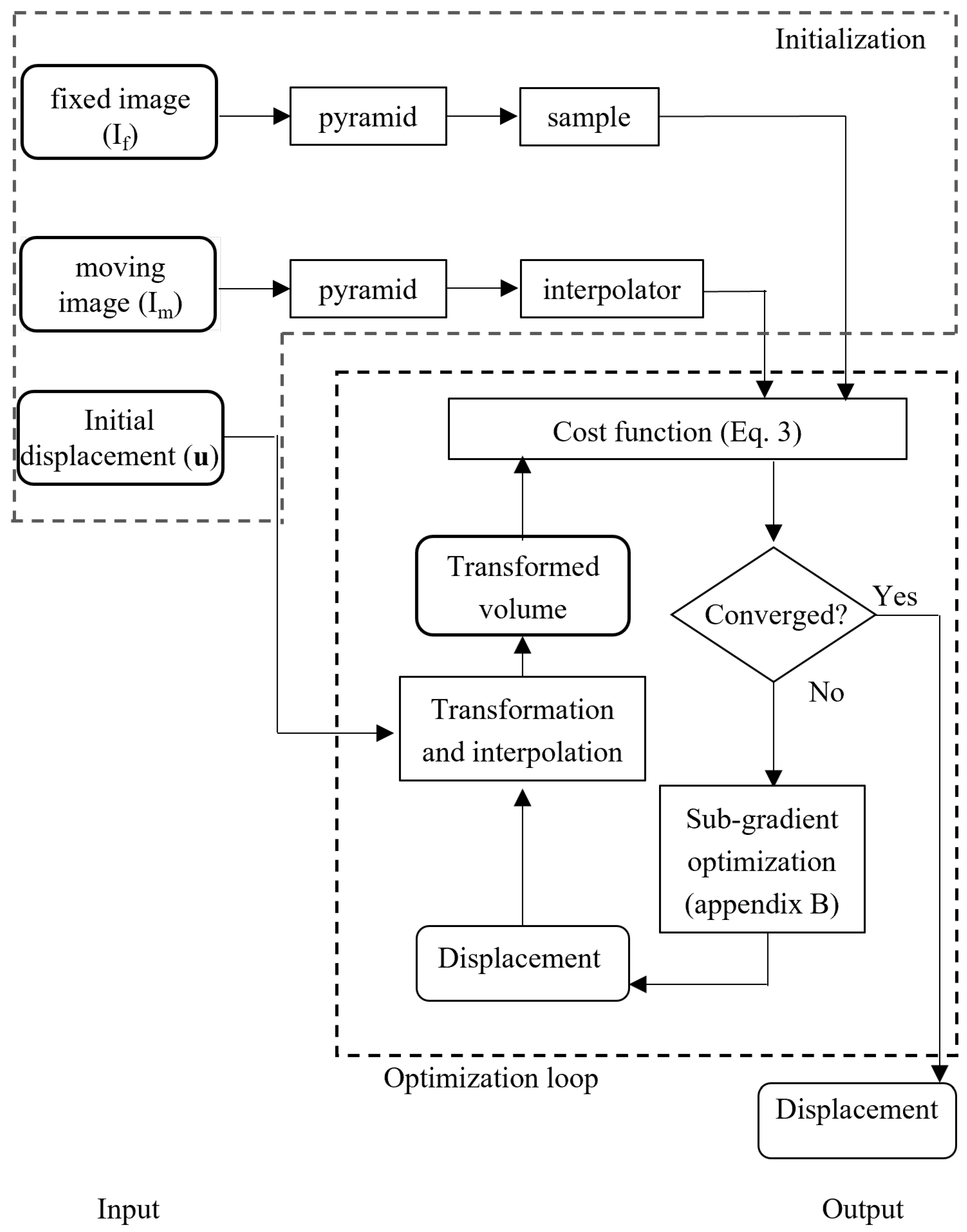
2.5. Implementation Details

The proposed DVC method takes as input the reference and the moving volume and the initial approximation of the displacement field (u). The initial displacement field, for the applications covered in this paper, is set to zero. In this work, a multi-resolution approach (i.e., pyramid approach) has been used. Such a method performs the registration at multiple resolution levels, in a coarse-to-fine sequence. Each level is defined by a different image resolution. The successive application of smoothing and subsampling operations helps to eliminate unnecessary details and mitigate aperture problems to disambiguate the motion’s direction. Besides the operation of smoothing and subsampling there is a reduction of the B-spline nodes spacing resolution. The number of pyramid levels and the relative grid spacing can be chosen based on the complexity of the motion to be described and on the structure’s size inside the material [42]. The grid spacing is usually not defined below 4 × 4 × 4 voxels, otherwise it is possible to incur in the folding effect, because the transformation has too much freedom.

For the applications reported in this paper, we used a Gaussian pyramid approach; at each level the image is smoothed (Gaussian blur) and subsampled by a factor of 2 in every direction. A schematic overview of the implemented DVC method is provided in Figure 2.

3. Datasets

As highlighted in Section 1, accurately characterizing cracks and interfaces in materials often necessitates modelling a high-resolution strain field with minimal noise [10,20]. Hence, the proposed method was employed to measure the strain near the cracks, and the obtained results were compared against those achieved through conventional smoothing techniques.

Specifically, two datasets were utilized in this study: one simulated and one experimental.

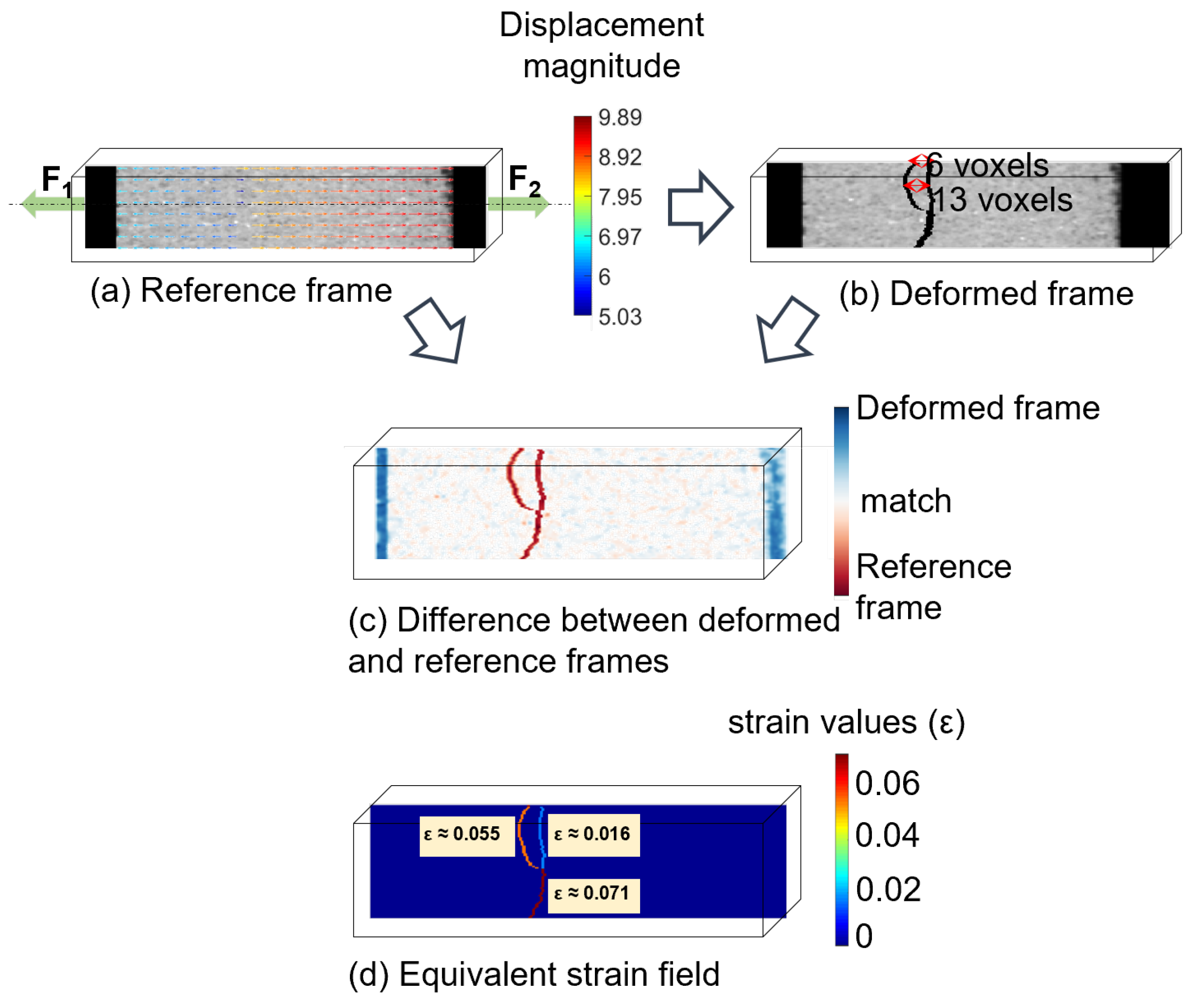
By utilizing a simulated dataset, our intention was to recreate the experimental configuration of cracks proposed in [10], which consists of a crack with two closely positioned branches, Figure 3.

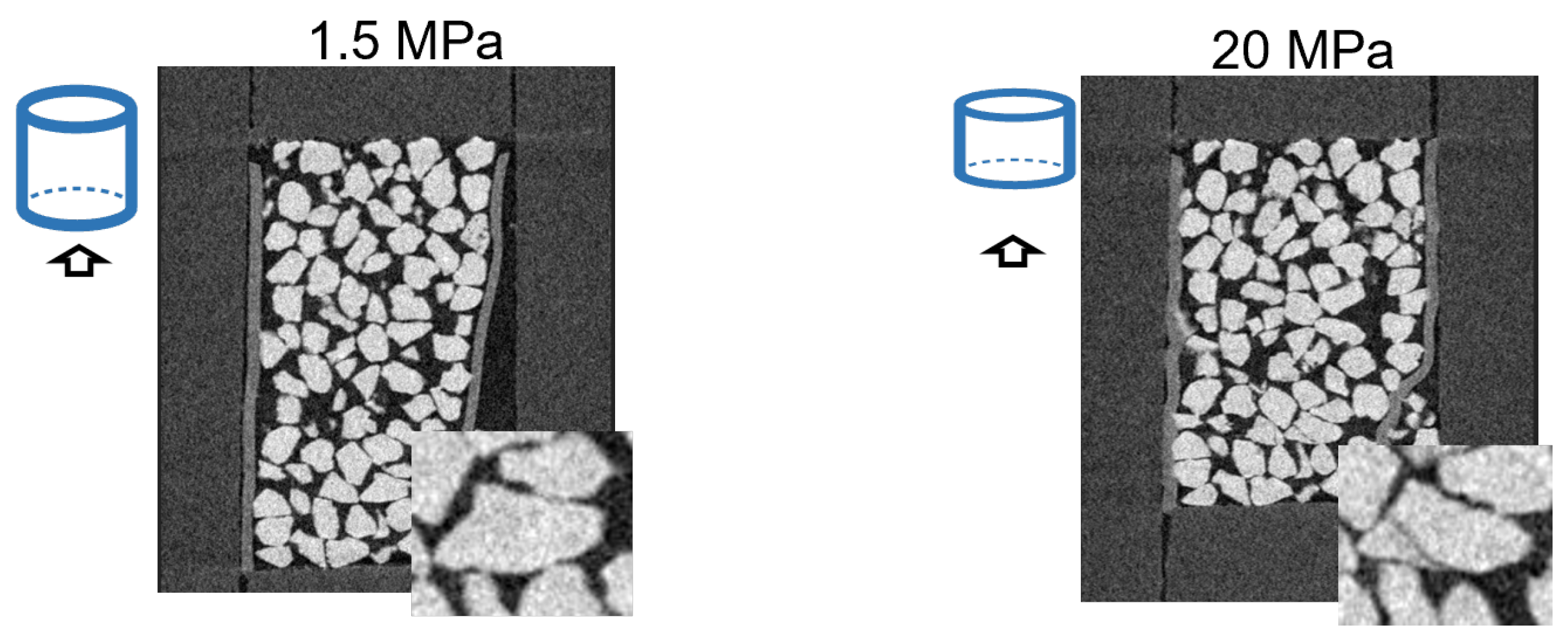
The experimental dataset was obtained through the compaction of an aggregate quartz grain sample, resulting in the presence of numerous cracks within the quartz grains due to the applied compression, Figure 4.

Further details regarding both datasets will be provided in the following subsections.

3.1. Simulated Data

The simulation involved generating a crack with two close branches induced by two forces pulling the two short lateral faces of the sample (Figure 3). The displacement field of a material that breaks is characterized by abrupt variations in magnitude and direction in the region around the crack [43]. Thus, we did not consider the material’s mechanical properties but instead simulated a displacement field that is compatible with crack formation, characterized by abrupt changes in the displacement field and resulting in peaks within the strain field (see Figure 3c).

The simulated dataset has a dimension of $230\times 100\times 50$ voxels, and the strain field contains very localized discontinuities associated with peaks. To perform the DVC process, we used a multi-resolution approach with four levels of a Gaussian pyramid, with the top-level B-spline node spacing equal to 8 voxels (×2 at each higher pyramid level). We set the value of the regularization parameter ${\lambda }_{TV}$ to 0.1.

3.2. Experimental Data: Aggregate Grain Sample

We utilized a 4D quartz sand dynamic dataset acquired during a uni-axial compaction experiment [44] (Figure 4). The dataset is available through the Yoda portal of Utrecht University [45] and was acquired using the Environmental Micro CT scanner (EM-CT) [46]. During the $\mu$-CT scans, 800 projections were taken over 360° at 120 KV acceleration voltage and 8 W output power. The voxel size was set to $5^3$ $\mathsf{\mu }$m, and volume reconstruction was performed using the Octupus software [47]. The sample had a diameter of 2 mm, with initial length varying between 1.4–2.5 mm. A compression was performed at different loads between 1.5 MPa and 50 MPa, resulting in ten scans. The first measured quartz grain breakage occurred at 20 MPa.

4. Results

In the results section, we aim to assess two key aspects of the proposed method: the increased accuracy of the computed strain field in the areas with cracks, compared to the classical techniques, and the algorithm’s performance as a crack detector.

Since the experiment with the quartz dataset is a real and non-destructive one, we lack a ground truth to directly compare the strain field with. Unlike the simulated dataset, where we have access to a reference measurement, this comparison is not possible in the case of the quartz dataset. The accuracy analysis for the simulated dataset has been carried out by calculating the mean absolute strain error (MAE). The numerical results can be found in the Section 4.2.

In the case of the real experiment, our only prior knowledge about the strain field is that areas with cracks exhibit high strain. Therefore, the only quantitative evaluation we can perform is to assess the strain within the crack areas. To accomplish this, we compare the number of voxels belonging to the cracks with the number of voxels corresponding to the high-strain area in the strain field.

The evaluation of a crack detector’s effectiveness typically involves comparing its output to the actual crack pattern obtained through manual or automatic segmentation of the cracks [10]. This allows for the estimation of true positive, true negative, false positive, and false negative detections, which in turn provides an assessment of the algorithm’s sensitivity.

4.1. Crack-Detection Methodology

The crack points are identified by detecting peaks in the strain field. Provided that the signal-to-noise ratio is sufficiently high, cracks can be detected by setting a strain threshold ($T_{ϵ}$) above the maximum elastic strain characteristic of the material. Additionally, the strain threshold must be higher than the strain noise level to ensure accurate crack detection [10]. However, it should be noted that the computed strain values are not equivalent to actual physical strain, which is zero in the crack area. Instead, the strain values are relative to the displacement of the crack lips, which can be used to identify cracks by applying a strain threshold.

In the crack-detection experiments (simulated dataset and aggregate grain sample), the equivalent von Mises strain was computed from the strain field obtained as by-product of the DVC algorithm. The equivalent strain takes into account all the strain components and simplifies the strain to a single scalar value

$$\begin{array}{cc}{ϵ}_{Mises}\hfill & =\frac{2}{3}[{ϵ}_{xx}^2+{ϵ}_{yy}^2+{ϵ}_{zz}^2-{ϵ}_{xx}^2{ϵ}_{yy}^2-{ϵ}_{xx}^2{ϵ}_{zz}^2-{ϵ}_{zz}^2{ϵ}_{yy}^2+\hfill \\ & +\frac{3}{4}({({ϵ}_{xy}+{ϵ}_{yx})}^2+{({ϵ}_{xz}+{ϵ}_{zx})}^2+{({ϵ}_{zy}+{ϵ}_{yz})}^2){]}^{\frac{1}{2}}\hfill \end{array}$$

(6)

4.2. Numerical Experiment Results

As an initial outcome, we will present a comparison between the accuracy of the strain field computed using our method and the median filter method. To the best of our knowledge, the utilization of median filters is a widely employed technique for noise removal in strain fields involving cracks, both in commercial and open-source software. This method is preferred due to its ability to preserve edges, unlike many other approaches. Additionally, since we aimed to replicate the crack configuration achieved by [10] and they specifically utilized the median filter technique, outlining its limitations, we sought to conduct a direct comparison between the two methods.

In order to examine the impact of the median filter window size, three distinct window sizes were investigated (w = $7,15,31$). The computed strain fields were compared with the simulated ground truth through both qualitative assessment using images and profile inspection (Figure 5), as well as quantitative evaluation using the mean absolute strain error (MAE) calculation. It has been found that the error obtained by applying TV-reg is much lower than the error obtained by using any other analyzed method. Based on the MAE values, the strain field that exhibits the highest deviation from the simulated one is the one obtaining after filtering the displacement field using a median filter with a window size of 31. The improvement in MAE obtained with TV-reg is $75.5\%$ compared to the DVC without regularization and $51.2\%$, $55.45\%$, and $83.10\%$ compared respectively to smooth-reg with window size equal to 7, 15, and 31.

When evaluating crack detection, the presence of noise poses a challenge in determining an optimal threshold that can accurately identify cracks while excluding noise. This difficulty becomes evident when working with the raw strain field without any regularization or filtering. In Figure 5b, the effect of three different threshold levels is reported. $T{1}_{ϵ}={10}^{-3}$ is evidently under the level of the noise; $T{2}_{ϵ}=2.2\times {10}^{-3}$, instead, highlights clearly the cracks location, but residual noise, that might lead to a misinterpreted crack detection, is still visible; $T{3}_{ϵ}=4\times {10}^{-3}$, instead, is likely to be too high to properly detect the crack location.

If we examine the strain field obtained after applying the median filter, we can observe that imposing a threshold value of $T1$ for window sizes of 7 and 15 leads to the detection of noise as an additional branch of the crack (see Figure 5c). On the other hand, when using a window size of 31, the two branches of the crack are not detected as separate branches. Applying a threshold of $T3$, only one of the two branches is detected in all cases (w = $7,15,31$). The only solution to accurately detect the cracks is by setting the threshold value to $T2$.

In the case of the strain field computed using TV regularization, the accuracy of crack detection is independent of the chosen threshold.

4.3. Aggregate Grain Compaction Experiment Results

TV-regularization has been used to detect cracks in $\mu$-CT images of an aggregate grain sample, formed as result of a compaction experiment. Moreover, in this case, the results have been compared to the performances of DVC without regularization and filtering operation and with smooth filtering. In order to detect cracks from the strain field a threshold value has been set ($T_{ϵ}=2\%$): the peaks of the strain field above $T_{ϵ}$ are considered to be caused by a crack in the grain. In Figure 6, one slice of the strain field computed without regularization (a), one with smooth regularization (b) and one with TV regularization (c) are shown.

In this application, the presence of noise in the strain field leads to numerous false positive detections. The noise peaks not only have similar amplitude to the actual strain, but they also exhibit similar crack openings (5–12 voxels). For instance, the crack labeled as number 1 has an opening of nine voxels, as indicated by the dashed rectangle in Figure 6e. That makes it impossible to distinguish a real crack from the noise. To enhance the sensitivity of the detection, we also evaluated a commonly employed median filtering technique [48,49] called smooth-reg. For this specific application, a window size of five voxels was chosen for the filter. However, it is important to note that this window size is still insufficient to completely eliminate all noise-induced peaks, and simultaneously compromises the spatial resolution, as it is visible from the strain profile (Figure 6e). The strain field computed using TV regularization demonstrates reduced variations around zero in the crack-free area compared to the strain field computed using the median filtering technique. In Figure 6c, four distinct peaks of high strain are visible, corresponding to the presence of four cracks.

Table 2. The range of the number of voxels attributed to the 28 cracks within the aggregate quartz grain sample.

Segmented	TV-Reg	Smooth-Reg
336–11 550	420–15 129	660–23 250

displays a comparative analysis of the number of voxels representing cracks segmented from the images and the corresponding number of voxels representing high strain areas in the strain field, as computed using the two methods.

TV-Reg Sensitivity Analysis

The impact of the threshold on the sensitivity of TV-reg for crack detection has been evaluated, Figure 6g. Such an analysis has been carried out based on a limited amount of annotated data. The ground truth has been created by manually annotating the grains with cracks. The labelling process has been performed by using the Image Labeler MATLAB app; we counted 73 quartz grains and 28 of them with cracks. The performances in terms of accuracy and sensitivity of TV-reg method have been compared with the results obtained by using smooth filtering and no strain field regularization and filtering. Eight levels of $T_{ϵ}$ have been analyzed, starting from 1.040 (left side of the graph in Figure 6g) to 1.005 (right side of the graph in Figure 6g) with an interval of 0.005. The noise in the solution without regularization plays an important role at every $T_{ϵ}$, resulting in the false positive rate (FPR) values that are for each $T_{ϵ}$ worse that in the smooth-reg and TV-reg. The sensitivity of TV-reg and smooth-reg is comparable at high levels of threshold (initial part of the curve). The smoothing process indeed reduces the noise level and thus limits false positive detections. However, in such a range the true positive rate (TPR) for smooth-reg and TV-reg is still too low for automatic crack detection. For higher values of TPR, the TV-reg is able to maintain a lower FPR compared to smooth-reg. The false positive detections with TV-reg are due to regions with high nominal strain, such as in a region where two grains are moving apart very quickly.

5. Discussion

In the previous section, a comparison was made between the results obtained using the proposed method and those obtained using the median filtering technique to reduce noise in the displacement field and, consequently, in the computed strain field. For the simulated dataset, which provided a strain field ground truth, a more comprehensive analysis was conducted. This analysis focused on a typical scenario where the requirements of high strain field resolution and low noise are crucial, particularly in the detection of cracks with multiple branches [10]. Specifically, the investigation encompassed various aspects, including the accuracy of the obtained strain field with and without additional noise in the input images, the data-fit accuracy at different values of lambda ($\lambda$), and the accuracy of crack detection.

• strain field and crack detection accuracy: The accuracy of the strain field and the effectiveness of the algorithm as a crack detector are interconnected.
  As anticipated, the strain field computed without regularization and without filtering exhibits high levels of noise. In this case, the noise amplitude is comparable to the strain associated with actual cracks, posing a challenge in determining an appropriate threshold level. The objective is to retain the high strain signal resulting from cracks while excluding high strain values caused by noise. It is noteworthy from the results obtained using the TV-reg method that the impact of noise on crack detection is limited, irrespective of the threshold level employed, Figure 5d,g. Using the median filter, accurate crack detection was achieved only with $T2$. A similar crack configuration was analyzed by [10], where the authors emphasized the impact of median filter window size on the detection of small crack spacings. Smaller filter sizes lead to a greater ability to detect smaller gaps between cracks. In our experiment, the reduction in detectable crack spacing becomes evident when using a small filter size (w = 7), particularly in the upper section of the image where the distance between the two branches is approximately six voxels, as shown in Figure 3 and Figure 5c. The filtered output with w = 7 produces unrealistic results, including the appearance of additional false branches caused by noise. Decreasing w from 7 to 5, which is smaller than the distance between the two branches, would prevent the two branches from connecting at the top. However, the increased noise would result in even less accuracy compared to w = 7.
  Additionally, the application of filtering operations alters the magnitude of the strain field, leading to a loss of valuable information regarding the real strain magnitude. Two factors contribute to the degradation of the MAE (

  Table 3. MAE of the strain values computed with TV-reg and smooth-reg (median filtering [10]).

  TV-Reg	Smooth-Reg (w = 7)	Smooth-Reg (w = 15)	Smooth-Reg (w = 31)
  $0.002$	$0.011$	$0.011$	$0.029$

  ) when median filtering is employed instead of the TV-reg method. Firstly, the presence of noise in the background. Secondly, the actual cracks area appears blurred. This implies that the median filter tends to include some voxels from the background in the crack area. The influence of these two factors varies based on the chosen window size. When the window size is smaller, the noise has a greater impact on the degradation of the MAE. Conversely, with a larger window size, the influence of the noise diminishes, while the impact of blurring becomes more significant (Figure 5, as shown in Table 3).
• data-fit: The optimization of the cost function, which consists of a similarity metric and the TV regularization term, involves finding a balance between data fit (measured by the similarity metric) and strain discontinuity. This balance is controlled by the parameter $\lambda$. The significant improvement in MAE (Figure 5h) justifies the choice of using TV regularization with lambda set to 0.1 instead of no regularization. Although the NCC metric, used to assess registration quality, shows a slightly higher value ($0.15\%$) in this case, Figure 7a. When $\lambda$ exceeds 0.1, the NCC (Normalized Cross-Correlation) value decreases significantly and becomes unreliable, making it unsuitable for consideration.

In the second experiment, due to the unavailability of a ground truth strain field, our main objective was to investigate the accuracy of crack detection. This was achieved by comparing the volumes of detected cracks using the two methods and assessing the sensitivity of crack detection. However, both the measurements of cracks volume and crack detection sensitivity serve as indicators of the accuracy of the computed displacement field. The observed shift towards higher values in the volume range of the smooth-reg method (Table 2) indicates the blurring effect and the resulting loss of information caused by classical smoothing techniques.

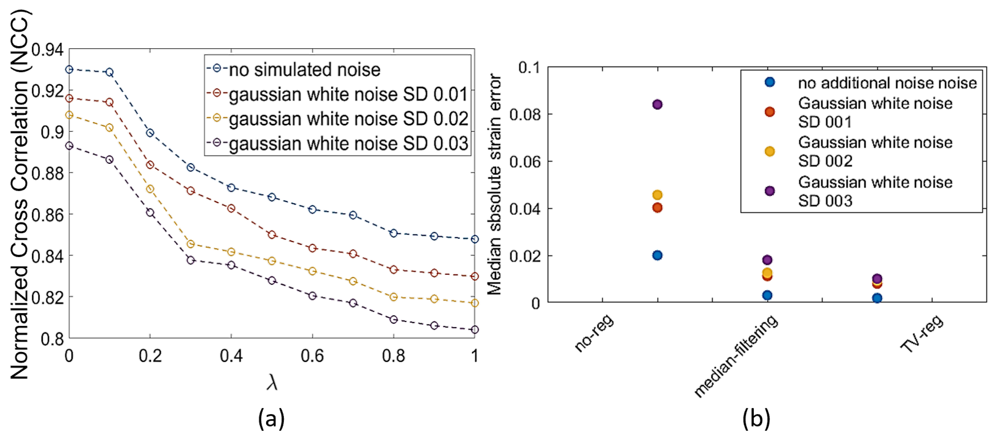
TV-reg has also been tested with noisy simulated input images. Indeed, together with the correlation errors, the causes of the noise in the displacement field is the quality of the input images [17]. Therefore, a degradation of the input images was simulated by adding Gaussian white noise with standard deviation (SD) ranging from 0.01 to 0.03. With an increase in the noise the performance of DVC decreases (Figure 7a) with and without regularization. In the case of the strain field computed with TV-reg, there is a substantial improvement in MAE, as shown in Figure 7b. When the strain field is derived from input images corrupted by Gaussian white noise with standard deviations of $0.01$, $0.02$, and $0.03$, the improvements in MAE are $71.46\%$, $74.60\%$, and $56.11\%$, respectively. These values are calculated by taking the average of five measurements. The noise on the input images has less impact if the strain field is computed using TV-reg instead of smooth-reg. This is because, with increased noise in the input images, more aggressive filters are required to mitigate the noise in the strain field. However, employing such filters comes at the expense of reduced spatial resolution, ultimately resulting in information loss.

6. Conclusions

In this study, we propose a novel regularization technique for DVC that utilizes the total variation of the strain field to estimate a sharp strain field capable of accurately describing abrupt deformations. Unlike classical denoising techniques that impose unrealistic assumptions on the dynamic behavior of materials, such as spatial smoothness in proximity to fractures, our proposed method does not require the use of post-processing noise-reduction techniques. The high signal-to-noise ratio of the computed strain field using our approach represents a significant advancement in crack detection. We demonstrate that the proposed TV-reg method is highly robust, as it reduces the risk of false crack detections, regardless of the chosen threshold. Furthermore, our method enhances the accuracy of the computed strain field, even in the presence of noisy input data, as depicted in Figure 7. These results were obtained following only a comparison with the widely recognized median filter technique, which, unlike other methods mentioned in Section 1, is available in open-source DVC software.

Although the proposed method was demonstrated to be highly robust, it is important to note that the method, due to its inherent design, is not universally applicable to all DVC problems. Its primary purpose is to measure the strain field in scenarios involving abrupt deformations. The key characteristic of this method lies in its definition of a piecewise constant strain and its utilization of trilinear B-spline transformation. However, the restricted degree of the B-spline function limits its suitability for applications requiring the estimation of smooth displacement and strain fields. Therefore, prior knowledge about the nature of the deformation is essential before applying this method. Furthermore, the proposed regularization technique for DVC is based on the assumption that the strain remains constant within the different structures of the material under a constant external stress. While this approximation is well-suited for the applications described in this paper, it may not always hold true in other scenarios. Thus, our method is most effective when the geometry of the material under stress is regular or can be approximated as such. To address this limitation, future developments of the algorithm could incorporate the geometric properties of objects to enhance its applicability in a wider range of scenarios.