Hyperspectral Anomaly Detection Based on Multi-Feature Joint Trilateral Filtering and Cooperative Representation

Abstract

The hyperspectral anomaly detection algorithm based on collaborative representation does not fully utilize the two-dimensional spatial features in hyperspectral images. It also has the problem that anomalous pixels will pollute the background dictionary and induce bad detection performance. Based on these, this paper proposes a hyperspectral anomaly detection algorithm based on multiple feature joint trilateral filtering and collaborative representation. The algorithm first introduces an improved trilateral filtering algorithm, which utilizes the spatial features of hyperspectral images. The preliminary positions of possible abnormal objects are determined. On this basis, abnormal removal and background filling are performed to obtain a purified background. Finally, the purified background and the original hyperspectral image are used for joint collaborative representation to complete the detection. Experimental results show that the detection accuracy of the algorithm proposed in this paper was efficiently improved by introducing multiple feature joint trilateral filtering, where multiple spatial spectrum features are utilized.

1. Introduction

As an important research direction in the field of remote sensing detection, hyperspectral image object detection has broad application prospects in environmental pollution monitoring, geological exploration, agriculture, forestry monitoring, etc. [1,2]. Hyperspectral detection can be divided into hyperspectral object detection and anomaly detection according to whether prior spectral knowledge of the object is required or not. In the actual situation, it is very difficult to obtain prior information due to the difficulty in obtaining accurate reflection spectrum of ground objects and the lack of a complete spectrum library. Commonly, the reflection spectrum of the anomaly objects is very different from that of the backgrounds, and the anomaly objects are small in the images. Therefore, the anomaly detection algorithm based on these features, without prior information, has much more application prospects in practice and attracts more attention compared to hyperspectral object detection. Thus, more and more attention is paid to the anomaly detection algorithms.

Among the hyperspectral anomaly detection algorithms, one of the most representative is the Reed–Xiaoli (RX) algorithm [3]. Based on the premise that the background part of the hyperspectral images is subject to a multivariate Gaussian distribution, the reference background mean vector and covariance matrix parameters are estimated by using the spectral vector mean of the hyperspectral image. Finally, the Markov distance between a single pixel and the statistical features of the reference background are calculated as the basis for the final judgment. The RX algorithm shows good detection performance in the hyperspectral images with a relatively simple background. However, it is difficult to correctly describe the various ground features of a complex hyperspectral dataset and noise interference. In view of the shortcomings of the RX algorithm, relevant researchers have also proposed correspondingly improved methods in different aspects [4,5,6,7,8]. Matteoli et al. effectively combined the kurtosis-driven binary hypothesis test with the RX algorithm to reduce the impact of the local covariance matrix calculation problem in the RX algorithm on the detection accuracy [4]. Gao et al. improved the RX algorithm by introducing an adaptive threshold to separate abnormal objects, which also effectively improved the detection performance [5]. Other improved algorithms with better effects include the fast RX detection algorithm based on heterogeneous clustering [6,7,8], the multi-window RX anomaly detection algorithm that uses windows of different sizes to describe different size anomaly objects to solve the problem of window size sensitivity in local anomaly detection [7], and the detection algorithm that further uses RX to effectively fuse spatial spectral features after expanding the multi-attribute profile to extract spatial features [8].

In 2015, the collaborative representation method was applied to the field of hyperspectral image anomaly detection (CRD) for the first time by Li et al. [9]. Compared with the RX algorithm, this algorithm does not make a Gaussian assumption for the background. It proposes that the background pixel can be approximately represented by the surrounding pixel, while the abnormal pixel cannot. Thus, the center pixel can be reconstructed by using the adjacent pixels. The algorithm uses the sliding double windows to obtain the background dictionary. Thus, the background dictionary is composed of some representative background pixels around the central pixel. The approximate value of the central pixel can be obtained through the linear combination of the background dictionary atoms. The distance between the central pixel and its approximate value is used to determine whether the central pixel is abnormal or not. The CRD algorithm usually shows excellent anomaly detection performance. However, its detection performance is limited to a certain extent because it only considers the spectral features of the hyperspectral images and does not make use of the spatial features of the hyperspectral images. At the same time, there is also the pollution problem of abnormal pixels in the background dictionary. Thus, the algorithm based on collaborative representation and other methods was also optimized to some extent by relevant researchers in later works [10,11,12,13,14,15,16,17].

The anomaly detection algorithm based on cooperative representation has the problem of insufficient utilization of the spatial features of the hyperspectral images, and the abnormal pixels also cause great interference to the background reconstruction. Therefore, an anomaly detection algorithm based on multi-feature joint trilateral filtering and cooperative representation (MFTFCR) was proposed in this paper. Firstly, an improved trilateral filter was introduced to obtain the abnormal points in the image by utilizing the spatial features of hyperspectral images. Then, the background purification of the hyperspectral image was completed. The purified image data and the original hyperspectral data are used for collaborative representation to complete the reconstruction of the hyperspectral image. Finally, the anomaly detection is completed according to the corresponding reconstruction error. The comparative experiment with other classical anomaly detection algorithms under different experimental data show that the algorithm in this paper has good anomaly detection ability. The algorithm proposed in this paper shows improved performance by introducing the multiple spatial spectral features of the hyperspectral images into collaborative representation.

2. Materials and Methods

2.1. Data

In order to accurately verify the performance of the algorithm, three hyperspectral image datasets are used for simulation experiments: Beach_Plane, Saliens_Synthetic, and Road_Vehicle. The Beach_Plane dataset is collected by an airborne visible/infrared spectral imager (AVIRIS), as shown in Figure 1. They are taken from the Cat Island beach, Australia, with a spatial resolution of 17.2 m/pixel. The 188 spectral bands are reserved, and the size of the spatial part is 140 × 140 after interception. The image mainly includes surface objects such as the sea surface, beach, and island, among which the abnormal objects are aircraft on the sea surface. The Saliens_Synthetic dataset is the synthetic experimental data shown in Figure 2. The real background image was taken by AVIRIS in the Salinas region, CA, USA, with a spatial resolution of 3.7 m/pixel. Its original hyperspectral image data size is 512 × 217, including 224 bands. The backgrounds are vegetable garden, land, vineyard, and other different types. In the experiment, a total of 204 bands, including 1~107, 113~153, and 168~223, were reserved. The 120 × 140 sized area was selected and embedded with 12 abnormal objects. The Road_Vehicle experimental dataset is taken by AVIRIS, and the suburban roads imaging scene is shown in Figure 3. The space size of this data after being intercepted from the original hyperspectral data is 100 × 100. The number of spectral bands is 186. The Road_Vehicle experimental dataset mainly includes road, grass, trees, and other ground objects. The abnormal objects are three vehicles on the road.

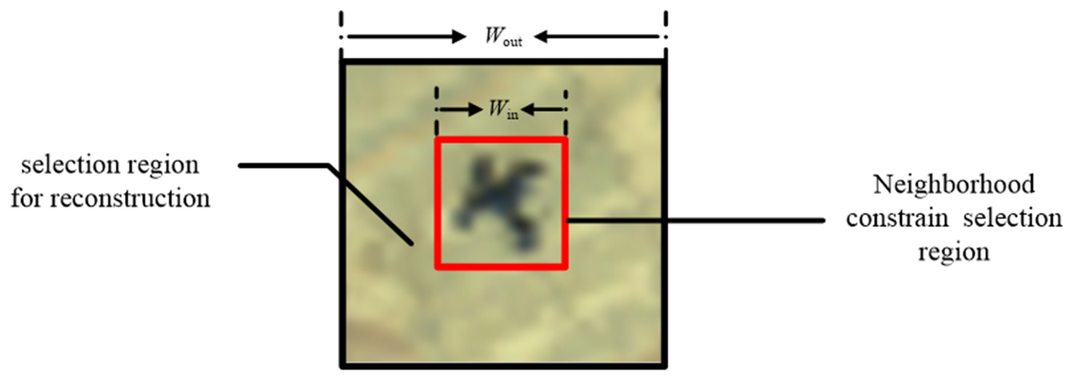
2.2. Anomaly Detection Algorithm Based on Cooperative Representation

Similar to the anomaly detection based on sparse representation, the background was reconstructed through the background dictionary for the anomaly detection algorithm based on cooperative representation. Then, the error was determined between the reconstruction and the original image. The anomaly detection method based on cooperative representation considers that the local background in the hyperspectral image has certain similarities. Thus, the background can be approximately replaced by the surrounding background components. By introducing the double-window structure (Figure 4), the pixels between the two windows are formed into the background dictionary to reconstruct the central image. The size of the inner window is W_in and the size of the outer window is W_out. The number of pixels between the inner and outer windows is num_{_b} = W_out × W_out − W_in × W_in. It is assumed that the pixels between the inner and outer windows belong to the background pixels, which construct the background dictionary A^b. The corresponding weight coefficient of the dictionary is x, and the central pixel based on the dictionary A^b can be expressed as A^bx. The reconstruction error can be defined as Equation (1).

$$\mathit{E}(\mathit{y})={‖\mathit{y}-{\mathbf{A}}^b\mathit{x}‖}_2$$

(1)

where E(y) is the error between the central pixel and the approximate value based on the dictionary representation. When the error is less than the threshold value, it is regarded that the central point to be measured is the background. Otherwise, it is the abnormal object.

For the cooperation-based anomaly detection method, the key problem to be solved is to find the optimal weight coefficient x, which can minimize the error E(y) under the constraint of the $\Vert \mathit{x}{\Vert }_2$ minimum. The mathematical description is Equation (2):

$$\underset{\mathit{x}}{\arg \min } {‖\mathit{y}-{\mathbf{A}}^b\mathit{x}‖}_2^2+\lambda {‖\mathit{x}‖}_2^2$$

(2)

where λ is the Lagrange multiplier. Furthermore, the equation can be expressed in Equation (3).

$$\underset{\mathit{x}}{\arg \min } \left[{\mathit{x}}^T\left({\left({\mathbf{A}}^b\right)}^T{\mathbf{A}}^b+\lambda \mathbf{I}\right)\mathit{x}-2{\mathit{x}}^T{\left({\mathbf{A}}^b\right)}^T\mathit{y}\right]$$

(3)

Take the derivative of the weight coefficient x and make the derivative 0. Then, x can be expressed in Equation (4).

$$\mathit{x}=\left({\left({\mathbf{A}}^b\right)}^T{\mathbf{A}}^b+\lambda \mathbf{I}\right){\left({\mathbf{A}}^b\right)}^T\mathit{y}$$

(4)

where I expresses the identity matrix.

When reconstructing the central pixel, it is considered that the weight coefficients can be different for various atoms of the background dictionary, to approach the central point value to be measured as close as possible. When the atoms in the dictionary are close to the point to be measured, a large weight coefficient is hoped. Otherwise, a small coefficient should be given. Thus, the dictionary is expressed in Equation (5).

$${\Gamma }_y=\left[\begin{array}{ccc}{‖\mathit{y}-{\mathit{a}}_1‖}_2& & 0\\ & \ddots & \\ 0& & {‖\mathit{y}-{\mathit{a}}_{num\_b}‖}_2\end{array}\right]$$

(5)

where a₁, a₂, …, a_{num_b} are the column vectors of the dictionary A^b, ${\Vert \mathit{y}-{\mathit{a}}_i\Vert }_2$ is the Euclidean distance between the point to be measured and the dictionary atom. Let y = [y; 1] and A^b = [A^b; 1]. Then, “1” is the length of the horizontal quantity of num_b. All the vector elements are 1. The sum of x is set to 1 to enhance the stability of the algorithm. Then, there will be Equation (6).

$$\underset{}{\arg \underset{x_1}{\min }{‖\mathit{y}-{\mathbf{A}}^b{\mathit{x}}_1‖}_2^2+\lambda {‖{\mathsf{\Gamma }}_{\mathit{y}}{\mathit{x}}_1‖}_2^2}$$

(6)

x can be expressed in Equation (7) by further solving Equation (6).

$${\mathit{x}}_1={\left({\left({\mathbf{A}}^b\right)}^T{\mathbf{A}}^b+\lambda {\mathsf{\Gamma }}_{\mathit{y}}{}^T{\mathsf{\Gamma }}_{\mathit{y}}\right)}^{-1}{\left({\mathbf{A}}^b\right)}^T\mathit{y}$$

(7)

After the above solution is obtained, the reconstruction error can be calculated according to Equation (1). Compared with the threshold th, the anomaly detection based on cooperative representation can be completed. The judgment process is expressed in Equation (8).

$$\mathit{E}(\mathit{y})={‖\mathit{y}-{\mathbf{A}}^b{\mathit{x}}_1‖}_2\left\{\begin{array}{l}\ge th Abnormal pixel\\ <th Background\end{array}\right.$$

(8)

2.3. Proposed Method

As discussed above, the anomaly detection algorithm based on cooperative representation has the problem of insufficient utilization of the spatial features of the hyperspectral images. Therefore, an anomaly detection algorithm based on multi-feature joint trilateral filtering and cooperative representation, i.e., MFTFCR, was proposed in this paper. With the help of an improved trilateral filter, the spatial features of hyperspectral images can be utilized, and the abnormal pixels are obtained in the image in advance. Then, the background purification of the hyperspectral image was completed. The purified image data and the original hyperspectral data are used for collaborative representation to complete the reconstruction of the hyperspectral image. Finally, the anomaly detection is completed according to the corresponding reconstruction error. Here, the multi-feature joint trilateral filtering and the background purification were expounded in detail.

2.3.1. Improved Trilateral Filtering Algorithm Based on Multi-Feature Combination

The trilateral filtering algorithm is widely used in the fields of noise suppression and image enhancement [18]. Compared with bilateral filtering, trilateral filtering takes into account the local structure features of the image, and better noise suppression or image enhancement effects can be achieved. Based on this, the trilateral filtering algorithm is introduced in this paper to reduce the algorithm pollution effect caused by anomalies in a collaborative representation by taking advantage of the spatial features of hyperspectral images.

As the spatial distribution of hyperspectral images also has a certain continuity, there is a certain similarity between the adjacent pixels. The closer the distance between two points, the greater the possibility of similar attributes. Therefore, it can be considered that the neighborhood pixels that are close to the center should also have greater weight coefficients in the representation process. The first term for improved trilateral filtering is given based on the spatial Euclidean distance weight (SEDW). It is expressed in Equation (9).

$$SEDW(x,\epsilon )=\exp \left(-\frac{1}{2}{\left(\frac{d_{sedw}(x,\epsilon )}{{\sigma }_{sedw}}\right)}^2\right)$$

(9)

where the coordinate of the center point x is (i, j), ε is the coordinates of the neighborhood point (i₁, j₁); σ_sedw is a parameter used to control the contribution of spatial Euclidean distance weight coefficient; and d_sedw represents the Euclidean distance between two points, which is expressed in Equation (10).

$$d_{sedw}(x,\epsilon )=\sqrt{{(i-i_1)}^2+{(j-j_1)}^2}$$

(10)

In the field of digital image processing, it is considered that the closer the gray magnitude of the neighborhood pixel and the center pixel, the more similar the two points are. Thus, a high weight coefficient should also be given in the reconstruction process. However, in hyperspectral images, the spectral curve vector is more important for each pixel point in space. The spectral curve reflects the true attribution of the object, and the difference between spectral curves can more reflect the difference between different points in hyperspectral images. Therefore, the second term in the improved trilateral filtering is given based on the spectral vector difference weight (SVDW), expressed in Equation (11).

$$SVDW(x,\epsilon )=\exp \left(-\frac{1}{2}{\left(\frac{d_{svdw}(x,\epsilon )}{{\sigma }_{svdw}}\right)}^2\right)$$

(11)

where σ_svdw is a parameter used to control the contribution of spectral vector difference weight coefficients; and d_svdw represents the spectral vector difference between two points. The expression is in Equation (12).

$$\begin{array}{c}{d}_{svdw}(x,\epsilon )=\frac{1}{\pi }\times \arccos \left({\displaystyle \sum _{i=1}^n\frac{{(x_i)}^T{\epsilon }_i}{\sqrt{{(x_i)}^T{x}_i}\sqrt{{({\epsilon }_i)}^T{\epsilon }_i}}}\right)\\ +\frac{1}{2}\times \left(1-\frac{{\displaystyle \sum _{i=1}^n(x_i-\overline{x})({\epsilon }_i-\overline{\epsilon })}}{\sqrt{{\displaystyle \sum _{i=1}^n{(x_i-\overline{x})}^2}}\sqrt{{\displaystyle \sum _{i=1}^n{({\epsilon }_i-\overline{\epsilon })}^2}}}\right)\end{array}$$

(12)

where, ε_I and x_i are the i-th elements in the corresponding spectral curve for the neighborhood points ε and the center point x and n is the number of spectral bands.

For hyperspectral image processing, the effective use of spatial features is also an essential part. The gradient feature is one of the most important features in two-dimensional space. In hyperspectral images, the gradient feature effectively represents the shape and smoothness of different types of objects. Therefore, the third term of the improved trilateral filtering is given, which is based on the local gradient difference (LGD), and it is expressed in Equation (13).

$$LGD(x,\epsilon )=\exp \left(-\frac{1}{2}{\left(\frac{d_{lgd}(x,\epsilon )}{{\sigma }_{lgd}}\right)}^2\right)$$

(13)

where σ_Lgd is a parameter used to control the contribution of the local gradient difference to the weight coefficient and d_lgd represents the local gradient value difference between two points. It is expressed in Equation (14).

$$d_{lgd}(x,\epsilon )=\mathbf{G}(x)-\mathbf{G}(\epsilon )$$

(14)

where G is the gradient value at position (i, j), and it is expressed in Equation (15).

$$\mathbf{G}\left(\mathbf{F}(i,j)\right)=\sqrt{{\left(\frac{\mathbf{F}(i,j+1)-\mathbf{F}(i,j-1)}{2}\right)}^2+{\left(\frac{\mathbf{F}(i+1,j)-\mathbf{F}(i-1,j)}{2}\right)}^2}$$

(15)

where F is the image used to calculate the gradient. In this paper, the principal component corresponding to the largest value of the hyperspectral image after PCA dimensionality reduction is used as the original two-dimensional image F.

In the above, combined with the features of hyperspectral image data, three weighting factors based on spatial Euclidean distance, spectral vector difference and two-dimensional spatial local gradient difference are given, respectively, from the joint perspective of spatial and spectral features. Based on these three weight calculation methods, the mathematical expression of improved trilateral filtering combined with multiple features is expressed in Equation (16).

$$\mathbf{R}(x)=\frac{1}{k(x)}\left({\displaystyle \sum _{i=1}^n\mathbf{O}({\epsilon }_i)SEDW(x,{\epsilon }_i)SVDW(x,{\epsilon }_i)LGD(x,{\epsilon }_i)}\right)$$

(16)

where x is the center pixel, ε_I is the neighborhood point, n is the number of neighborhood points of x, O is the image before reconstruction, and R is the image after filtering. k(x) is the regularization parameter and is expressed in Equation (17).

$$k(x)={\displaystyle \sum _{i=1}^{n}SEDW(x,{\epsilon }_i)}SVDW(x,{\epsilon }_i)LGD(x,{\epsilon }_i)$$

(17)

2.3.2. Background Purification

The improved trilateral filter can be helpful in the reconstruction of the background part. A large reconstruction error will be expected while using the neighborhood background atom to represent the abnormal part. Based on this principle, the preliminary abnormal information distribution can be obtained. When the central pixel is the background component, the weight coefficient for the similar background components will be large when reconstructing the representation, and the reconstruction error is small. However, when the central pixel is an abnormal pixel, the weight coefficient for the background component will be small, and that for the abnormal pixels will be large, resulting in a smaller reconstruction error. In this situation, the preliminary extraction of anomaly information cannot be obtained according to the above principles. Many studies were carried out to solve similar problems [7,8,9,10,11]. The internal and external double-window structure was introduced to restrict the selection of reconstructed atoms. As shown in Figure 4, the abnormal pixel occupies a small part of the hyperspectral image, and also has a certain degree of aggregation. Thus, the influence of the abnormal neighborhood pixels on the reconstruction results is greatly reduced by adding the inner frame limit area and selecting the corresponding pixels between the inner and outer windows for reconstruction.

After adding the area limit, the size of the inner window may be set to W_in, and the size of the outer window may be set to W_out. Equation (16) can be updated to Equation (18):

$$\mathbf{R}(x)=\frac{1}{k(x)}\left({\displaystyle \sum _{i=1}^N\mathbf{O}({\epsilon }_i)SEDW(x,{\epsilon }_i)SVDW(x,{\epsilon }_i)LGD(x,{\epsilon }_i)}\right)$$

(18)

where O is the initial feature image, R is the background image after filtering and reconstruction, x is the central pixel, ε_i represents the i-th pixel of the reconstructed selection region between the inner and outer windows, and k(x) is the corresponding regularization parameter, which can be updated to Equation (19).

$$k(x)={\displaystyle \sum _{i=1}^{N}SEDW(x,{\epsilon }_i)}SVDW(x,{\epsilon }_i)LGD(x,{\epsilon }_i)$$

(19)

where N is the number of reconstructed pixels between the inner and outer windows, and the calculation formula is expressed in Equation (20).

$$N=W_{out}\times W_{out}-W_{in}\times W_{in}$$

(20)

After the background reconstruction of the initial feature image is completed by sliding through the whole image with two windows, further operations are performed on the initial feature image and the filtered background image to obtain the reconstruction representation error. It is expressed in Equation (21).

$$\mathbf{E}(x)=\mathbf{I}(x)-\mathbf{R}(x)$$

(21)

when E(x) is greater than a certain threshold, the pixel can be considered as a possible abnormal point, and when it is lower than the threshold, the pixel can be considered the background point. After traversing the whole image, the coordinates of all possible abnormal points should be recorded. Then, the spectral curve at the corresponding coordinates of the possible abnormal points will be set to zero in the original hyperspectral image and replaced by the mean vector of all possible background pixels in the neighborhood. In order to ensure the effectiveness of the filling vector, the size of the filling neighborhood is consistent with the size of the previous internal window (W_in) to complete the background purification. Then, the purified background and the original image are used to complete the joint collaborative representation. The background parts between the two windows in the purified background image are used as dictionary atoms to reconstruct the central pixel. Finally, the final detection result is obtained according to the reconstruction error between the pixel to be measured and the reconstructed spectral curve.

3. Results and Discussion

For a comparison, seven classic hyperspectral anomaly detection algorithms, RX [3], local RX(LRX) [19], CRD [9], Whitening Special Correlation Filtering (WSCF) [20], Robust Principal Component Analysis Based on Reed-Xiaoli (RPCA-RX) [21], Low-Rank and Sparse Representation (LRASR) [22], and Kernel Isolation Forest-based hyperspectral anomaly Detection(KIFD) [23] are selected. The advantages and disadvantages of the algorithms of this paper are further analyzed by comparing the detection results of different algorithms. The experimental simulation was carried out on the Windows10 operating system with MATLAB R2018b software and i3 8300 processor (Intel, Santa Clara, CA, USA).

3.1. Beach Analysis of the Plane Image Experiment Results

(1)

Parameter setting

This experimental data include the sea surface, beach, island, aircraft, and other objects. One aircraft on the sea surface is the abnormal object and the rest is the background. For the algorithm of this paper, the main parameters involved are the parameters σ_sedw, σ_svdw, and σ_Lgd that control the corresponding output sensitivity in the improved trilateral filtering. There is also the threshold th for possible exception objects, which cooperatively represent regularization parameters λ, and the corresponding size of the inner (W_in) and outer windows (W_out). It is verified by experiments that it has little effect on the final result, and it is uniformly set to 10⁻⁶ for the regularization parameter λ in the collaborative representation. The parameters in the improved trilateral filtering σ_sedw, σ_svdw, and σ_Lgd are set to be 5, 5, and 1. The size of the inner and outer windows, W_in and W_out, are 13 and 17, and the threshold th is set to 0.9.

(2)

Results and discussion

The experimental simulation results of each algorithm on the Beach_Plane images are shown in Figure 5. Figure 5a shows the true value of the abnormal objects corresponding to the dataset, and Figure 5b–i shows the abnormal detection results of each comparison algorithm and the algorithm of this paper. In Figure 5, all algorithms can detect abnormal objects. However, the shape contour of abnormal objects in the detection results of the LRX algorithm is not as clear as other algorithms. In terms of background suppression, the algorithms of this paper, the LRX algorithm and CRD algorithm, have good background suppression effects, while the LRASR and KIFD algorithms have poor background suppression effects on this dataset, with a large number of obvious background residues. This indicates that there will be obvious false alarms for the LRASR and KIFD algorithms while not for the proposed algorithm.

In order to observe the test results more clearly, the three-dimensional display of the test results is further analyzed subjectively on the basis of Figure 5. Figure 6 shows the corresponding 3D display of the test results. Figure 6a shows the three-dimensional distribution of real abnormal objects, and Figure 6b–i shows the three-dimensional grid corresponding to the detection results of all the algorithms. In the 3D grid of the experimental results in Figure 6, it can be seen clearly that the LRX algorithm has the best background suppression effect. However, the amplitude of some abnormal objects is small for this algorithm, and the degree of abnormal object retention is slightly worse than other algorithms. The serious background residue can be observed by the LRASR algorithm on this dataset. The object detection property of the KIFD algorithm is the best, but there are still many island background residues. In the detection results of the RX, CRD, WSCF, RPCA-RX, and the algorithms of this paper, the detection of abnormal objects is obvious. The amplitude in the background region of the CRD algorithm and the algorithm of this paper is relatively small, which indicates a good background suppression effect. The amplitude in the background region of other comparison algorithms is relatively large, and thus the background suppression effect of them is not as good as that of the CRD algorithm and the algorithm of this paper. Compared with the contrast algorithm, the algorithm of this paper has better subjective visual effects on object detection and background suppression in this experimental dataset.

Further quantitative parameter analysis and evaluation was carried out on the detection results of the algorithms of this paper and comparison algorithms. The corresponding subject feature curves (ROC curves) of all algorithms on the Beach_Plane experimental dataset are shown in Figure 7, and the AUC values of the area under the corresponding curve are shown in

Table 1. AUC values for Beach_Plane dataset.

Algorithm	RX	LRX	CRD	WSCF	RPCA-RX	LRASR	KIFD	Ours
AUC	0.9852	0.9971	0.9943	0.9840	0.9787	0.9621	0.9910	0.9981

.

In the ROC curve result diagram in Figure 7, when the false alarm rate is less than 0.05, the difference between the algorithms, except the LRASR algorithm, is small. When the false alarm rate is close to 0.05, the detection probability of the algorithm of this paper is rapidly improved. The detection probability is larger than that of other comparison algorithms under the fixed false alarm rate. At the same time, the algorithm of this paper reaches the detection probability of one at the earliest time. Based on the summary of AUC values in Table 1, it can be seen that the AUC value of the algorithm of this paper is obviously higher than those of the RX, WSCF, RPCA-RX, and LRASR algorithms. LRX, CRD, KIFD and the algorithm of this paper show good detection performance, with AUC values above 0.99.

3.2. Experiment Results of the Saliens_Synthetic Image

(1)

Parameter setting

In this experimental dataset, the scene includes vegetable garden, land, vineyard, and other ground object categories, including 12 synthetic anomaly objects. λ is set to be 10⁻⁶ for the regularization parameter in the collaborative representation. The parameters in the improved trilateral filtering σ_sedw, σ_svdw, and σ_Lgd are set to be 3, 3, and 3. The size of the inner and outer windows, W_in and W_out, are 13 and 15, and the threshold th is set to 0.3.

(2)

Results and discussion

The experimental results on this experimental dataset are shown in Figure 8. Figure 8a shows the true value of the abnormal object, and Figure 8b–i shows the abnormal detection results corresponding to all algorithms. As can be seen from Figure 8, the LRX and CRD algorithms can only detect part of the objects in the experimental data, and the detected object contour size and other information are seriously lost. In the detection results of the RX, WSCF, and RPCA-RX algorithms, the object detection degree is poor, and some smaller objects are not obvious. The LRASR and KIFD algorithms can detect all objects, and the brightness of the detected objects is large, which indicates good detection properties. However, there are obvious background residues in the detection results of these two algorithms, indicating the false alarm detected by these algorithms. Compared to other contrast algorithms, the residual background was greatly reduced for the algorithm of this paper, and at the same time the relevant information such as the contour of the object is preserved while detecting all the objects.

Figure 9a shows the 3D map of the real abnormal object, and Figure 9b–i shows the 3D grid map corresponding to the detection results of all algorithms. In Figure 9, the amplitude of each part can be clearly observed. In this experimental dataset, the LRX and CRD algorithms have a good background suppression effect, while there are missing cases of some objects. In the detection results of RX, WSCF, and RPCA-RX algorithms, the peak value at each object location is small, indicating that the object detection is not obvious. The LRASR and KIFD algorithms still have large numerical peaks outside of the object, and there are many background residues. The amplitude at each object location is large, and there is no large numerical peak residue outside of the object location for the algorithm of this paper, indicating good object detection and background suppression performance in comparison with other algorithms.

The results of each algorithm are further analyzed and evaluated quantitatively. The corresponding ROC curves are shown in Figure 10, and the corresponding AUC values are shown in

Table 2. AUC values of the Saliens_Synthetic dataset for all algorithms.

Algorithm	RX	LRX	CRD	WSCF	RPCA-RX	LRASR	KIFD	Ours
AUC	0.9858	0.9541	0.9363	0.9869	0.9925	0.9713	0.9965	0.9998

. In Figure 10, compared to other comparison algorithms, the ROC curve of the algorithm of this paper is closer to the upper left corner of the coordinate axis, indicating that the detection probability of the algorithm of this paper is better than that of the comparison algorithms under various false alarm rates. At the same time, the AUC values of RPCA-RX, KIFD, and the algorithm of this paper, are greater than the AUC values of other comparison algorithms in Table 2. The LRX, CRD, and LRASR algorithms show relatively poor detection performance.

3.3. Road_Analysis of Vehicle Image Experiment Results

(1)

Parameter setting

In this dataset, the image mainly includes road, grass, trees, soil, cars, and other ground objects, of which three smaller objects on the road are abnormal objects, and the rest are background components. Λ is set to 10⁻⁶ for the regularization parameter in the collaborative representation. The parameters in the improved trilateral filtering σ_sedw, σ_svdw, and σ_Lgd are set to be 5, 5, and 5. The size of the inner and outer windows, W_in and W_out, are 7 and 9, and the threshold th is set to be 0.3.

(2)

Results and discussion

The experimental results on this dataset are shown in Figure 11. The true value diagram of the abnormal object is shown in Figure 11a, and the detection results of the comparison algorithms and the algorithm of this paper are shown in Figure 11b–i. In Figure 11, all algorithms do not miss the abnormal detection. In the detection diagram of the RX and RPCA-RX algorithms, the detection effect of the abnormal objects in the middle is not obvious. At the same time, the RX, LRX, WSCF, RPCA-RX, and KIFD algorithms have more obvious yellow highlights on the right side of the image, indicating the obvious false alarm. The object detection effect of the LRASR algorithm is good, but there are some background residues on the left side of the image. The background suppression effect of the KIFD algorithm is poor, and the object detection is not obvious. In the detection results of the CRD algorithm and the algorithm of this paper, the obvious false alarm phenomenon on the right side of the image and the background residual phenomenon on the left side are better than other algorithms. The object shape in the CRD algorithm is significantly different from the real object, and the contour shape of the object detected by the algorithm of this paper is closer to the contour shape of the real object in the truth map.

Figure 12a–i shows the 3D grid corresponding to the real abnormal object and the detection results of all the algorithms. In Figure 12, it can be clearly seen that the amplitude of the abnormal object position in the middle is small in the detection results of the RX and RPCA-RX algorithms, indicating that the detection effect is not good. In the detection results of the RX, WSCF, and RPCA-RX algorithms, the residual parts of the road near the abnormal object are obvious. The LRASR algorithm can detect three abnormal objects well, but there are some background residues at the edge of the image. The overall amplitude of the KIFD algorithm detection result is large, indicating poor background suppression. The right part of the detection results of the RX, LRX, and WSCF algorithms has a large numerical peak, corresponding to the relatively significant false alarm. The amplitude of the three objects is large for the algorithm of this paper. The false alarm and background residues are relatively small.

The results of all the algorithms are further analyzed and evaluated quantitatively. The corresponding ROC curves are shown in Figure 13, and the corresponding AUC values are shown in

Table 3. AUC values of the Road_Vehicle dataset for all algorithms.

Algorithm	RX	LRX	CRD	WSCF	RPCA-RX	LRASR	KIFD	Ours
AUC	0.9909	0.9992	0.9946	0.9988	0.9902	0.9997	0.8908	0.9997

. It can be seen from the enlarged part in the upper left corner of Figure 13 that the detection probability of the algorithm of this paper and LRASR algorithm is higher than that of other comparison algorithms under certain false alarm rates. The detection probability of the proposed algorithm reaches one at the earliest time. Based on Table 3, we can see that the algorithm of this paper and the comparison algorithms (except KIFD) have a large AUC value of more than 0.99. The algorithm of this paper and the LRASR algorithm have the highest value of 0.9997, indicating a good detection effect compared to other algorithms.

3.4. Overall Evaluation of the Experimental Results

Combined with the experimental results of three different real hyperspectral images, the algorithm of this paper has relatively good results in object detection, background suppression, and other aspects, compared to the seven algorithms for comparison in subjective evaluation. It shows fewer false alarms and no large area of false detection. In terms of objective evaluation, the summary of AUC values of different algorithms in three datasets is shown in

Table 4. AUC values of all algorithms for three experimental sets of data.

	Beach_Plane	Saliens_Synthetic	Road_Vehicle
RX	0.9852	0.9858	0.9909
LRX	0.9971	0.9541	0.9992
CRD	0.9943	0.9363	0.9946
WSCF	0.9840	0.9869	0.9988
RPCA-RX	0.9787	0.9925	0.9902
LRASR	0.9621	0.9713	0.9997
KIFD	0.9910	0.9965	0.8908
Ours	0.9981	0.9998	0.9997

. It can be seen from the table that the final detection parameters of RX, WSCF, and the proposed algorithm of this paper, show relatively excellent performance in different datasets. The other five algorithms can usually perform well on two datasets. As the proposed algorithm of this manuscript is based on CRD, the comparison between CRD and the proposed algorithm would be more significant. As can be seen from the table, obvious progress is obtained on the Saliens_Synthetic dataset and the AUC value increases from 0.9363 (CRD) to 0.9998 (ours). The above subjective and objective evaluation results verify the effectiveness of the algorithm of this paper.

3.5. Experiment on Another Dataset

Another experiment on the California_Airport dataset is provided. This dataset is collected by an airborne visible/infrared spectral imager from California’s Moffett Airport, with a wavelength range of 0.4–2.5 μm. Figure 14 shows the pseudo-color image of the experimental data and the true distribution position image of the abnormal targets. The spatial resolution is 3.5 m/pixel. The original hyperspectral image data size is 1924 × 753, including 224 bands. After removing some bands in the simulation, 178 bands, including 1–98, 113–114, 129–153, and 172–224, were used. A 192 × 48 sized area was selected for detection. The figure includes types of ground objects such as roads, soil, grasslands, airports, etc. Aircraft and maintenance vehicles at the airport are considered abnormal targets.

The experimental simulation results of each algorithm on the California_Airport dataset are shown in Figure 15. Figure 15a shows the true value of the abnormal objects corresponding to the dataset, and Figure 5b–i shows the abnormal detection results of each comparison algorithm and the algorithm of this manuscript. The AUC values of all the algorithms are shown in

Table 5. AUC values for California_Airport dataset detection.

Algorithm	RX	LRX	CRD	WSCF	RPCA-RX	LRASR	KIFD	Ours
AUC	0.9526	0.9821	0.9570	0.9427	0.9655	0.9081	0.9800	0.9667

. From Figure 15 and Table 5, it can be seen that LRX and KIFD show relatively good performance. They can detect all abnormal objects. Compared to these two algorithms, RX, WSCF, and the proposed algorithm in this manuscript, will miss some abnormal objects, which are circled in Figure 15i. In addition, there are also some false alarms for the proposed algorithm. These indicate that the proposed algorithm does not show a good detection performance, especially compared to LRX and KIFD in this dataset.

4. Conclusions

A hyperspectral anomaly detection algorithm based on multiple feature joint trilateral filtering and collaborative representation was proposed in this paper. With the help of an improved trilateral filter, the spatial features of hyperspectral images can be fully utilized, and the abnormal pixels are obtained in the image in advance. This helps to reduce the bad effect of abnormal pixels on the background reconstruction. Experiments were carried out on three hyperspectral images and seven detection algorithms were selected for comparison. The above subjective and objective evaluation results verify that some progress was achieved by introducing an improved trilateral filter based on cooperative representation, indicating the effectiveness of the algorithm in this paper.

References

1. Yuan, Y.; Wang, Q.; Zhu, G. Fast hyperspectral anomaly detection via high-order 2-D crossing filter. IEEE Trans. Geosci. Remote Sens. 2015, 53, 620–630. [Google Scholar] [CrossRef]
2. Wang, X.Y.; Wang, L.G.; Wang, J.W.; Sun, K.P.; Wang, Q.M. Hyperspectral Anomaly Detection via Background Purification and Spatial Difference Enhancement. IEEE Trans. Geosci. Remote Sens. 2022, 19, 6006005. [Google Scholar] [CrossRef]
3. Reed, I.S.; Yu, X. Adaptive multiple-band CFAR detection of an optical pattern with unknown spectral distribution. IEEE Int. Conf. Acoust. Speech Signal Process. 1990, 38, 1760–1770. [Google Scholar] [CrossRef]
4. Matteoli, S.; Diani, M.; Corsini, G. Hyperspectral anomaly detection with kurtosis-driven local convarience matrix corruption mitigation. IEEE Geosci. Remote Sens. Lett. 2011, 8, 532–536. [Google Scholar] [CrossRef]
5. Gao, L.; Guo, Q.; Plaza, A.; Li, J.; Zhang, B. Probabilistic anomaly detector for remotely sensed hyperspectral data. J. Appl. Remote Sens. 2014, 8, 083538. [Google Scholar] [CrossRef]
6. Melero, J.M.; Paz, A.; Garzon, E.M.; Martinez, J.A.; Plaza, A.; Garcia, I. Fast anomaly detection in hyperspectral images with RX method on heterogeneous clusters. J. Supercom. 2011, 58, 411–419. [Google Scholar] [CrossRef]
7. Liu, W.; Chang, C. Multiple-window anomaly detection for hyperspectral imagery. IEEE J. Sel. Topics Appl. Earth Observ. Remote Sens. 2013, 6, 644–658. [Google Scholar] [CrossRef]
8. Zhang, Y.; Hua, W.S.; Huang, F.Y.; Wang, Q.H.; Suo, W.K. Space-Spectrum Joint Anomaly Degree for Hyperspectral Anomaly Target Detection. Sectrosc. Spect. Anal. 2020, 40, 1902–1908. [Google Scholar]
9. Li, W.; Du, Q. Collaborative representation for hyperspectral anomaly detection. IEEE Trans. Geosci. Remote Sens. 2015, 53, 1463–1474. [Google Scholar] [CrossRef]
10. Xiang, P.; Zhou, H.X.; Li, H.; Song, S.Z.; Tan, W.; Song, J.L.Q.; Gu, L. Hyperspectral anomaly detection by local joint subspace process and support vector machine. Int. J. Remote Sens. 2020, 41, 3798–3819. [Google Scholar] [CrossRef]
11. Xie, W.Y.; Li, Y.S.; Lei, J.; Yang, J.; Chang, C.I.; Li, Z. Hyperspectral band selection for spectral-spatial anomaly detection. IEEE Trans. Geosci. Remote Sens. 2020, 58, 3426–3436. [Google Scholar] [CrossRef]
12. Qu, Y.; Wang, W.; Guo, R.; Ayhan, B.; Kwan, C.; Vance, S.; Qi, H.R. Hyperspectral anomaly detection through spectral unmixing and dictionary-based low-rank decomposition. IEEE Trans. Geosci. Remote Sens. 2018, 56, 4391–4405. [Google Scholar] [CrossRef]
13. Kang, X.; Li, S.; Benediktsson, J.A. Spectral-spatial hyperspectral image classification with edge-preserving filtering. IEEE Trans. Geosci. Remote Sens. 2014, 52, 2666–2667. [Google Scholar] [CrossRef]
14. Zhang, Y.; Fan, Y.; Xu, M.; Xu, M.M.; Li, W.; Zhang, G.Y.; Liu, L.; Yu, D.F. An improved low rank and sparse matrix decomposition-based anomaly target detection algorithm for hyperspectral imagery. IEEE J. Sel. Topics Appl. Earth Observ. Remote Sens. 2020, 13, 2663–2672. [Google Scholar] [CrossRef]
15. Ma, Y.; Fan, G.; Jin, Q.W.; Huang, J.; Mei, X.G.; Ma, J.Y. Hyperspectral anomaly detection via integration of feature extraction and background purification. IEEE Geosci. Remote Sens. Lett. 2021, 18, 1436–1440. [Google Scholar] [CrossRef]
16. Zhuang, L.; Gao, L.; Zhang, B.; Fu, X.Y.; Bioucas-Dias, J.M. Hyperspectral image denoising and anomaly detection based on low-rank and sparse representations. IEEE Trans. Geosci. Remote Sens. 2020, 60, 1–17. [Google Scholar]
17. Verdoja, F.; Grangetto, M. Graph Laplacian for image anomaly detection. Mach. Vision. Appl. 2020, 31, 11. [Google Scholar] [CrossRef] [Green Version]
18. Gao, Z.; Gu, C.; Yang, J.; Gao, S.S.; Zhong, Y.M. Random weighting based nonlinear gaussian filtering. IEEE Access. 2020, 8, 19590–19605. [Google Scholar] [CrossRef]
19. Matteoil, S.; Veracini, T.; Diani, M.; Corsini, G. A locally adaptive background density estimator: An evolution for RX-based anomaly detection. IEEE Geosci. Remote Sens. Lett. 2014, 11, 323–327. [Google Scholar] [CrossRef]
20. Gaucel, J.M.; Guillaume, M.; Bourennane, S. Whitening spatial correlation filtering for hysperspectral anomaly detection. In Proceedings of the IEEE International Conference on Acoustics, Speech, and Signal Processing, Philadelphia, PA, USA, 18–23 March 2005; pp. 333–336. [Google Scholar]
21. Wright, J.; Peng, Y.G.; Ma, Y. Robust principal component analysis: Exact recovery of corrupted low-rank matrices via convex optimization. Adv. Neural Inf. Process. Syst. 2009, 87, 3–56. [Google Scholar]
22. Yang, X.; Wu, Z.; Li, J.; Plaza, A.; Wei, Z.H. Anomaly detection in hyperspectral images based on low-rank and sparse representation. IEEE Trans. Geosci. Remote Sens. 2016, 54, 1990–2000. [Google Scholar]
23. Li, S.; Zhang, K.; Duan, P.; Kang, X.D. Hyperspectral Anomaly Detection with Kernel Isolation Forest. IEEE Trans. Geosci. Remote Sens. 2020, 58, 319–328. [Google Scholar] [CrossRef]
Figure 1. Beach_Plane experimental dataset. Pseudo-color image (a). Graph of true anomaly objects (b).
Applsci 13 06943 g001
Figure 2. Saliens_Synthetic experimental dataset. Pseudo-color image (a). Graph of true anomaly objects (b).
Applsci 13 06943 g002
Figure 3. Road_Vehicle experimental dataset. Pseudo-color image (a). Graph of true anomaly objects (b).
Applsci 13 06943 g003
Figure 4. Selected area for the reconstruction.
Applsci 13 06943 g004
Figure 5. Beach_Plane dataset detection results. Graph of true abnormal object (a); RX (b); LRX (c); CRD (d); WSCF (e); RPCA-RX (f); LRASR (g); KIFD (h); ours (i).
Applsci 13 06943 g005
Figure 6. Three-dimensional grid detection results of the Beach_Plane dataset. Graph of true abnormal object (a); RX (b); LRX (c); CRD (d); WSCF (e); RPCA-RX (f); LRASR (g); KIFD (h); ours (i).
Applsci 13 06943 g006
Figure 7. ROC curves of the Beach_Plane dataset detection results. ROC curves (a); Enlarged view of the upper left corner of ROC (b).
Applsci 13 06943 g007
Figure 8. Experiment results of the Saliens_Synthetic dataset. Graph of true abnormal object (a); RX (b); LRX (c); CRD (d); WSCF (e); RPCA-RX (f); LRASR (g); KIFD (h); ours (i).
Applsci 13 06943 g008
Figure 9. Three-dimensional grid detection results of the Saliens_Synthetic dataset. Graph of true abnormal object (a); RX (b); LRX (c); CRD (d); WSCF (e); RPCA-RX (f); LRASR (g); KIFD (h); 0urs (i).
Applsci 13 06943 g009
Figure 10. ROC curve of the Saliens_Synthetic dataset. ROC curves (a); Enlarged image of the top left of ROC curves (b).
Applsci 13 06943 g010
Figure 11. Detection results of the Road_Vehicle dataset. Graph of true abnormal object (a); RX (b); LRX (c); CRD (d); WSCF (e); RPCA-RX (f); LRASR (g); KIFD (h); ours (i).
Applsci 13 06943 g011
Figure 12. Three-dimensional grid detection results of the Road_Vehicle dataset. Graph of true abnormal object (a); RX (b); LRX (c); CRD (d); WSCF (e); RPCA-RX (f); LRASR (g); KIFD (h); ours (i).
Applsci 13 06943 g012
Figure 13. ROC curve of the Road_Vehicle dataset. ROC curves (a); Enlarged image of the top left of ROC curves (b).
Applsci 13 06943 g013
Figure 14. California_Airport experimental dataset. (a) Pseudo-color image; (b) Graph of true anomaly objects.
Applsci 13 06943 g014
Figure 15. California_Airport dataset detection results. Graph of true abnormal object (a); RX (b); LRX (c); CRD (d); WSCF (e); RPCA-RX (f); LRASR (g); KIFD (h); ours (i).
Applsci 13 06943 g015aApplsci 13 06943 g015b