Electromagnetic Imaging for Buried Conductors Using Deep Convolutional Neural Networks

Featured Application

Electromagnetic imaging. Featured applications include military measurements, medical imaging, industrial applications, underground gas pipe and electrical high-voltage cable detection, etc.

Abstract

In the past, many conventional algorithms, such as self-adaptive dynamic differential evolution and asynchronous particle swarm optimization, were used to reconstruct buried objects in the frequency domain; these were unfortunately time-consuming during the iterative, repeated computing process of the scattered field. Consequently, we propose an innovative deep convolutional neural network approach to solve the electromagnetic inverse scattering problem for buried conductors in this paper. Different shapes of conductors are buried in one half-space and the electromagnetic wave from the other half-space is incident. The shape of the conductor can be reconstructed promptly by inputting the received scattered fields measured from the upper half-space into the deep convolutional neural network module, which avoids the computational complexity of Green’s function for training. Numerical results show that the root mean square error for differently shaped—circular, elliptical, arrow, peanut, four-petal, and three-petal—reconstructed images are, respectively, 2.95%, 3.11%, 17.81%, 15.10%, 14.14%, and 15.24%. Briefly speaking, not only can circular and elliptical buried conductors be reconstructed; some irregular shapes can be reconstructed well. On the contrary, the reconstruction result by U-Net for buried objects is worse since it is not able to obtain a good preliminary image by processing only the upper scattered field—that is, rather than the full space. In other words, our proposed deep convolutional neural network can efficiently solve the electromagnetic inverse scattering problem of buried conductors and provide a novel method for the microwave imaging of the buried conductors. This is the first successful attempt at using deep convolutional neural networks for buried conductors in the frequency domain, which may be useful for practical applications in various fields such as the medical, military, or industrial fields, including magnetic resonance imaging, mine detection and clearance, non-destructive testing, gas or wire pipeline detection, etc.

1. Introduction

Electromagnetic inverse scattering (EMIS) is an important research subject, involving the physical phenomenology and mathematical modeling of electromagnetic wave signals reflected, scattered, and transmitted from the surface of a target object. The uncertainty of electromagnetic inverse scattering could be a major issue since the accurate description of the targeted shapes is essential for object identification and localization. However, in actual practice, target shapes are often unknown, uncertain, or even composed of multiple sub-targets. In order to overcome this barrier, more sophisticated techniques had to be introduced; the object was located wither in free space or half-space. The methods for solving inverse problems in free space can further be categorized into conventional iterative algorithms and deep learning (DL) methods. In the iterative algorithms method, Zheng proposed discrete dipole approximation to solve the inverse scattering problem for conductors according to the equivalence principle. The equivalent surface currents comprised numerous discrete dipole moments. The simulation results indicated that better imaging results, a circularly polarized wave was superior [1]. In 2022, Ye proposed an Iterative multiscaling approach, a subspace-based optimization method, and an inversion method for buried conductors’ image reconstruction. Note that he had considered both synthetic and experimental data in assessing the reconstruction accuracy [2].

In recent years, deep learning neural networks have developed rapidly in various fields. In 2015, Ronneberger proposed U-Net, which consists of a contracting path to capture context and a symmetric expanding path to enable precise localization on biomedical image segmentation applications [3]. There have been many successful applications, including electromagnetic calculations. To overcome the shortcut in nonlinear electromagnetic inverse scattering problems for dielectric objects in free space, in 2019, Wei proposed three training schemes, including direct inversion, backpropagation, and dominant current schemes, to calculate the initial image and then input it to U-Net to reconstruct the image [4]. In 2020, Guo applied an image translation network, named the complex-valued pix2pix, which included two parts: a generator and a discriminator. Results show that the complex-valued pix2pix could learn the mapping from the initial contrast to the real contrast in microwave imaging models [5]. In 2021, end-to-end scalable cascaded convolutional neural networks were proposed to solve ISP. High-resolution images could be obtained directly from the scattered field with the guiding of the multiresolution labels in the cascaded blocks [6]. In 2022, Chiu proposed the dominant current scheme and backpropagation scheme to calculate the preliminary permittivity distribution and then combine with U-Net to reconstruct the uniaxial objects [7]. However, these methods need the preliminary image; the reconstruction result by U-Net for buried objects is worse since it is not able to obtain good preliminary images by processing only the upper scattered field—that is, rather than the full space.

For buried objects under the frequency domain, most researchers applied conventional algorithms to solve the electromagnetic inverse scattering problems. In 2015, Lee proposed to use asynchronous particle swarm optimization to reconstruct permittivity of the two-dimensional inhomogeneous dielectric cylinder [8]. In 2019, Chiu proposed to use a self-adaptive dynamic differential evolution method to reconstruct the periodic homogeneous dielectric object buried in rough surfaces [9]. However, these methods will spend a lot of time in iterative calculation of the complex Green’s function. In 2020, Fan proposed an accurate and robust method to reconstruct buried objects for half-space scenarios. First, the linear sampling method (LSM) was employed to estimate the targets. A relaxed error threshold was defined for LSM to ensure all real targets had been included. Second, differential evolution optimization was used to refine the LSM results [10]. In 2022, Ren proposed a method for reconstructing media objects buried in three layers of media by using 2D projection as well as the shadow projections of 3D images. The proposed method could reconstruct the size and dimension of uniform objects significantly but could not identify the material of the object [11]. For neural network mechanisms, in 2021, Wan provided a robust and efficient data-based strategy for underground metal target detection on portable devices with limited computing capability and energy supply applications. This cross-combination strategy of dimensionality reduction methods and machine learning models provided a means to find the optimal machine learning model for underground target detection [12]. Nevertheless, it could not reconstruct the shape of the object.

One of the studies in half-space is using ground penetrating radar (GPR) to detect buried objects and earth layers by transmitting the electromagnetic wave time domain pulses of different frequencies. This also demonstrates that electromagnetic backscattering can be used in a wide range of applications such as military surveys, medical imaging, and industrial applications such as underground gas or electrical pipelines. In GPR, Lameri proposed a pipeline for buried landmine detection based on the convolutional neural network (CNN) and GPR images. The validation of the presented system was carried out on real GPR acquisitions, and it was possible to reach 95% of detection accuracy in 2017 [13]. In 2018, Sonoda and Kimoto developed a method for identifying subsurface objects from GPR images using deep neural networks in the time domain. In this study, features of subsurface objects were extracted and learned from generated GPR images by a 9-layer convolutional neural network. The results showed that the CNN could identify different materials with approximately 80% accuracy in heterogeneous subsurface media [14]. Ozkaya proposed a novel multilevel deep learning-based algorithm for GPR B-scan by buried object detection. An efficient layer-by-layer training approach was formulated to learn the deep dictionaries and different classifiers of types of shapes of buried objects [15]. However, it could not reconstruct the arbitrary shape of metal. In 2021, Ambrosanio investigated the recovery performance of a specific and unconventional contactless multistatic GPR system for the subsurface imaging of antitank and antipersonnel plastic mines [16]. In GPR application, Barkataki proposed a CNN model for predicting the size of buried objects from the GPR B-Scan. This method demonstrated good performance in predicting buried object sizes in 2022 [17]. In the above articles, only the position or size of the objects were being reconstructed, not the shape of the objects. In brief, GPR transmits time domain pulses of electromagnetic waves at various frequencies for buried objects and soil layers. Compared with GPR, we apply the time-harmonic field, which has only a single frequency, to transmit the electromagnetic waves. This implies that it would be more difficult to reconstruct the object in the frequency domain.

In this paper, we propose a seep convolutional neural network (DCNN) to solve the buried conductor in the frequency domain. We use the measured scattered fields as the input data to the DCNN for training. Different shapes of conductors are buried in one half-space and the electromagnetic is incident from the other half-space is incident. By inputting the received scattered fields measured from the upper half-space into the deep convolutional neural network module for training, the shape of the conductor can be reconstructed promptly. Most of the published articles in free-space apply U-Net, which requires an initial guess in the training process to reconstruct the image. However, since the object is buried in half-space, the performance of U-Net is poor because the lower part of the object cannot be measured. Numerical results present that our proposed method is efficient as well as timely compared with conventional methods. Since DCNN can avoid the computational complexity of the Green’s function, real-time imaging can be achieved in time as soon as the module is trained. To the best of our knowledge, DCNN implementation on buried conductors in the frequency domain is the first to be rolled out. In addition, we believe that it would have various beneficial practical applications in medical and military or industrial fields, including magnetic resonance imaging, mine detection and clearance, non-destructive testing, gas or wire pipeline detection, etc.

2. Forward Problem

Consider a perfect conductor buried in a lossy half-space, as shown in Figure 1. The permittivity and conductivity in Region I and Region II are $\left({\epsilon }_1,{\sigma }_1\right)$ and $\left({\epsilon }_2,{\sigma }_2\right)$, respectively. In each region, the permeability of free space is set to ${\mu }_0$; that is, only non-magnetic substances are considered. Let the scatterer be a cylindrical conductor extending infinitely in the z-axis. Its cross-sectional area in the $xy$-plane can be expressed by the equation $\rho =F\left(\theta \right)$. The time-varying relation of the incident wave is set to $e^{j\omega t}$ and its incident angle is ${\varnothing }_1$, as depicted in Figure 1.

For simplicity, the direction of the incident electric field is assumed to be parallel to the z-axis, which is the TM polarization wave direction. Using $E_i$ to represent the electric field distribution when the conductor is not present, $E_i$ can then be expressed as follows:

$${\overrightarrow{E}}_i\left(\overrightarrow{r}\right)=E_i\left(x,y\right)\widehat{z},$$

(1)

where

$$E_i\left(x,y\right)=\left\{\begin{array}{cc}{E}_1\left(x,y\right)=e^{-j{k}_1[xsin{\varnothing }_1+\left(y+A\right)cos{\varnothing }_1]}+R_1{e}^{-j{k}_1[xsin{\varnothing }_1-\left(y+A\right)cos{\varnothing }_1]}& ,y\le -A\hfill \\ E_2\left(x,y\right)=T{e}^{-j{k}_2[xsin{\varnothing }_2+\left(y+A\right)cos{\varnothing }_2]}& ,y>-A\hfill \end{array}\right.$$

(2)

$$R_1=\frac{1-n}{1+n} , T=\frac{2}{1+n} ,n=\frac{cos{\varnothing }_2}{cos{\varnothing }_1}\sqrt{\frac{{\epsilon }_2-j{\sigma }_2/\omega }{{\epsilon }_1-j{\sigma }_1/\omega }}$$

(3)

$$k_{1}sin{\varnothing }_1=k_{2}sin{\varnothing }_2$$

(4)

$$k_i^2={\omega }^2{\epsilon }_1{\mu }_0-jw{\mu }_0{\sigma }_i, i=1,2 Im\left(k_i\right)\le 0.$$

(5)

The first term, $E_1\left(x,y\right)$, is the so-called incident field $E^{inc}$. If Region I and Region II are the lossless media, then ${\varnothing }_1$ and ${\varnothing }_2$ represent the angle of incidence and refraction, respectively. On the contrary, if Region I and Region II are the lossy media, then ${\varnothing }_1$ and ${\varnothing }_2$ become more complex. The wave form will be very complicated. Its propagation direction will be different with the decay direction. The total electric field at any point in the space can be tabulated as follows:

$$E\left(x,y\right)=\left\{\begin{array}{c}{E}_1\left(x,y\right)+E_s\left(x,y\right)\hspace{1em},y\le -A\\ E_2\left(x,y\right)+E_s\left(x,y\right)\hspace{1em},y>-A\end{array}\right.,$$

(6)

where $E_s\left(x,y\right)$ is the scattered field. Since the size of our interested object is about one wavelength (i.e., in the resonance region), the scattered field will have a severe diffraction effect. In order to solve for a correct scattered field, we must first carefully calculate the Green’s function $G\left(x,y;x\prime ,y\prime \right)$ for this half-space problem. This can be generated by a line current source at $\left(x\prime ,y\prime \right)$ and the scattered field at $\left(x,y\right)$. Via the Fourier transform technique, $G\left(x,y;x\prime ,y\prime \right)$ can be expressed as follows:

$$G\left(x,y;x^{\prime },y^{\prime }\right)=\left\{\begin{array}{cc}{G}_1\left(x,y;x^{\prime },y^{\prime }\right)& ,y\le -A\hfill \\ G_2\left(x,y;x^{\prime },y^{\prime }\right)=G_f\left(x,y;x^{\prime },y^{\prime }\right)+G_s\left(x,y;x^{\prime },y^{\prime }\right)& ,y>-A\hfill \end{array}\right.$$

(7)

$$G_1\left(x,y;x^{\prime },y^{\prime }\right)=\frac{1}{2\pi }{{\displaystyle \int }}_{-\infty }^{\infty }\frac{j}{{\gamma }_1+{\gamma }_2}{e}^{j{\gamma }_1\left(y+A\right)}{e}^{-j{\gamma }_2\left(y^{\prime }+A\right)}{e}^{-j\alpha \left(x-x^{\prime }\right)}d\alpha .$$

(8)

The Green’s function matrix can be expressed as follows:

$$G_f\left(x,y;x^{\prime },y^{\prime }\right)=\frac{j}{4}{H}_0^{\left(2\right)}\left[k_2\sqrt{{(x-x\prime )}^2+{(y-y\prime )}^2}\right]$$

(8a)

$$G_s\left(x,y;x^{\prime },y^{\prime }\right)=\frac{1}{2\pi }{{\displaystyle \int }}_{-\infty }^{\infty }\frac{j}{2{\gamma }_2}\left(\frac{{\gamma }_2-{\gamma }_1}{{\gamma }_2+{\gamma }_1}\right)e^{-j{\gamma }_2\left(y+2A+y^{\prime }\right)}{e}^{-j\alpha \left(x-x^{\prime }\right)}d\alpha$$

(8b)

$$\begin{array}{c}{\gamma }_i^2=k_i^2-{\alpha }^2,\hspace{1em}i=1,2,\hspace{1em}Im({\gamma }_i)\le 0,\hspace{1em}y\prime >A\end{array}.$$

(9)

Conceptually, the scattered field $E_S\left(x,y\right)$ can be regarded as the surface induced current $J_s$ on the conductor radiating in the half-space. By means of and the two-dimensional Green’s function, the scattered field outside the conductor can be expressed as follows:

$$E_s=\left\{\begin{array}{c}-{{\displaystyle \int }}_0^{2\pi }{G}_1\left(\stackrel{\rightharpoonup }{r};F\left({\theta }^{\prime }\right),\theta \right)J\left({\theta }^{\prime }\right)d{\theta }^{\prime }\hspace{1em},y\le -A\\ -{{\displaystyle \int }}_0^{2\pi }{G}_2\left(\stackrel{\rightharpoonup }{r};F\left({\theta }^{\prime }\right),\theta \right)J\left({\theta }^{\prime }\right)d{\theta }^{\prime }\hspace{1em},y>-A\end{array}\right.,$$

(10)

where

$$\stackrel{\rightharpoonup }{r}=\left(x,y\right), J\left(\theta \right)=-j\omega {\mu }_0\sqrt{F^2\left(\theta \right)+F^{\prime 2}\left(\theta \right)}{J}_s\left(\theta \right).$$

(11)

The boundary condition for a perfect conductor is that the total electric field in the tangential direction on the surface of the conductor is zero. According to this boundary condition, we can obtain the integral equation of $J\left(\theta \right)$:

$$E_2\left(F\left(\theta \right),\theta \right)={{\displaystyle \int }}_0^{2\pi }{G}_2\left(F\left(\theta \right),\theta ;F\left({\theta }^{\prime }\right),{\theta }^{\prime }\right)J\left({\theta }^{\prime }\right)d{\theta }^{\prime }.$$

(12)

The scattered field in Region I is as follows:

$$E_s\left(x,y\right)=-\begin{array}{c}{{\displaystyle \int }}_0^{2\pi }{G}_1\left(x,y;F\left({\theta }^{\prime }\right),{\theta }^{\prime }\right)J\left({\theta }^{\prime }\right)d{\theta }^{\prime },\hspace{1em}y\le -A\end{array}.$$

(13)

3. Deep Convolutional Neural Network (DCNN) and Inverse Problem

DCNN is a DL method in machine learning, as shown in Figure 2. By imitating the mathematical model of the biological nervous system, multiple calculations and trainings of different levels and structures are performed to seek the optimal and most effective DL model. In contract to the past, where rules must be pre-defined by human beings for machine learning, DCNN only requires the finetuning of the training data and parameters in the designed neural network. The machine is capable of learning by itself to discriminate the features and then calculate the best result. The key to develop DCNN is to continuously provide high-quality data and perform computational training to produce better DCNN models. In order to accelerate the training process, advanced hardware platforms, such as the GPU (graphics processing unit), and improved software have been introduced. DCNN training can be regarded as a “heterogeneous” process that transfers the measured scattered field into a preliminary contrast of the object domain. The input in the DCNN framework consists of the real and imaginary parts of the objective contrast. The convolutional layer is a special neural layer used to extract features in the image. It converts each part of the image into a smaller feature vector by sliding a small matrix called a convolutional kernel over the image. The main advantage of the convolutional layer is that it can capture local patterns and textures in the image and can classify objects in the image regardless of their location. The activation layer is a layer that performs non-linear transformation of the feature vectors extracted from the convolutional layer to increase the representational power of the neural network. It usually uses the ReLU (rectified linear unit) function, which sets the negative values to 0 and keeps the positive values. This choice is made because ReLU can effectively prevent the gradient disappearance problem while maintaining computational efficiency. Finally, these feature vectors are fed into a fully-connected layer for the final classification or regression operation. This layer usually consists of multiple neurons, each of which is connected to some feature vectors in the preceding convolutional and activation layers. Through this combination, the neural network can learn to make associations between the extracted features and the desired output classes or values for reconstructing the image. We also try to use the most popular U-Net to reconstruct our images. As U-Net requires a preliminary image, the direct sampling method is utilized. However, in our experience, the initial preliminary image obtained solely from the upper scattered field, i.e., rather than from the full space of U-Net, would be bad. This is why we propose DCNN to reconstruct the buried conductor in this research.

We employed the measured scattered fields $E_s$ as the input data and put it into the DCNN module for training. The $M_i$ × $M_r$ × 2 matrix comprises the input data transformed from the scattered fields using $E_s$. $M_i$ represents the number of incident fields, $M_r$ represents the number of receivers, and the real and imaginary parts of $E_s$ will be split into two channels, as shown in Figure 2. Briefly speaking, comparing with the past conventional methods, using $E_s$ as the input value for the DCNN can cope with the EMIS problem efficiently.

The mean square error (MSE) is used as a loss function for training the DCNN model; it is the mean of the square differences between our target and predicted values and is defined as follows:

$$Loss=0.5\times {\displaystyle {{\displaystyle \sum }}_{n=1}^{WHC}}{\left({\tilde{y}}_n-y_n\right)}^2,$$

(14)

where W, H, and C denote the width, height, and number of channels of the output, respectively, and n presents the transmit number indexing, linearly, into each element of ${\tilde{y}}_n$ and $y_n$.

If the activation function is not used in the neural network, the input linear combination of the upper layer will be used as the output of this layer. In addition, the output and input are still inseparable from the linear relationship. In this way, we use the activation function to solve the nonlinearity issue. $w_i$ and $b_i$ represent the weights and bias in the layer, while $\delta \left(x\right)$ represents the activation function, which is the rectified linear unit (ReLU) described as follows:

$$\delta \left(x\right)=\left\{\begin{array}{c}0\hspace{1em}\hspace{1em}\hspace{1em}for x<0\\ x\hspace{1em}\hspace{1em}\hspace{1em}for x\ge 0\end{array}\right..$$

(15)

Figure 3 presents the flowchart of the complete experimental process. First, we place the conductors in a simulated environment. Then, the electromagnetic wave illuminates the buried conductors. Scattered field information with training and test data is inputted into DCNN for training. Upon DCNN training, test data are put into the trained DCNN for image reconstruction.

4. Numerical Result

In this section, a simulation environment in half-space (Figure 1) is designed to numerically analyze the inverse scattering problem of perfect conductors. The frequency of the incident wave is 3 GHz. The buried depth, A, is set to a wavelength (0.1 m). The background substance in Region 1 is air with ${\epsilon }_1={\epsilon }_0$ and ${\sigma }_1=0$; while the background substance in Region 2 is the soil with ${\epsilon }_2=2.56$, ${\epsilon }_0$ and ${\sigma }_2=0$. TM-polarized plane waves are emitted to illuminate the scatterers. As much as 5% Gaussian noises are added to the environment, and 32 receivers from $\theta =$ ${195}^{°}$ to ${350}^{°}$, with radius 3 m, and 32 transmitters from ${\varnothing }_1=$ $-{80}^{°}$ to ${80}^{°}$ with $5^{°}$ intervals are deployed. In short, a total of 32 receivers and 32 transmitters are placed in our simulated environment. We aim to utilize the received scattered field collected from various incident angles and input it to the DCNN to reconstruct the object.

In our simulated environment, we place the scatterer in the 32 × 32 pixel area. We assume that the scatterer has different sizes which can be located at any places within the measurement area. We simulate different shapes for various random positions. We then illuminate each profile with 32 different incident angles. The total number of dataset images is about 2000. They are split into two parts, in which 80% of the data is used for training and 20% for testing.

The high computational performance of GPU parallelization is well suited for training because each training is independent during the process. In the training option, we choose adaptive moment estimation (Adam) because it is commonly used in practice. Intuitively, Adam is a fusion of the adaptive gradient algorithm (Adagrad) and momentum; it has the advantage of bias correction so as to limit the learning rate for each iteration, allowing the parameters to be updated more smoothly. Meanwhile, we set the initial learning rate at 10⁻⁵ and drop the learning rate by half at every 70 epochs. The momentum parameter is set at 0.99, the batch size is 32, and the max epoch is 200. We will shuffle the data upon each epoch trained in the DCNN training process. This is due to the strong fitting capability of DCNN. In other words, the order of the samples may be cached if the same combination of batches appears repeatedly, which could affect the generalization outcome.

In order to calculate the performance of each scheme, we define the root mean square error (RMSE) formula as follows:

$$RMSE=\frac{1}{M}{\displaystyle {{\displaystyle \sum }}_{i=1}^M}\Vert Y-Y^i{\Vert }_F/\Vert Y{\Vert }_F,$$

(16)

where Y and Yⁱ denote the true shape and the reconstructed shape, respectively, M is the total number of tests, and F is the Frobenius norm.

In order to compare the reconstruction results of each graph trained by the neural-like network, we define the structural similarity index measure (SSIM) as follows:

$$SSIM=\frac{\left(2{\mu }_{\tilde{y}}{\mu }_y+C_1\right)\left(2{\sigma }_{\tilde{y}y}+C_2\right)}{\left({\mu }_{\tilde{y}}^2+{\mu }_y^2+C_1\right)\left({\sigma }_{\tilde{y}}^2+{\sigma }_y^2+C_2\right)}.$$

(17)

For SSIM details, please refer to reference [7].

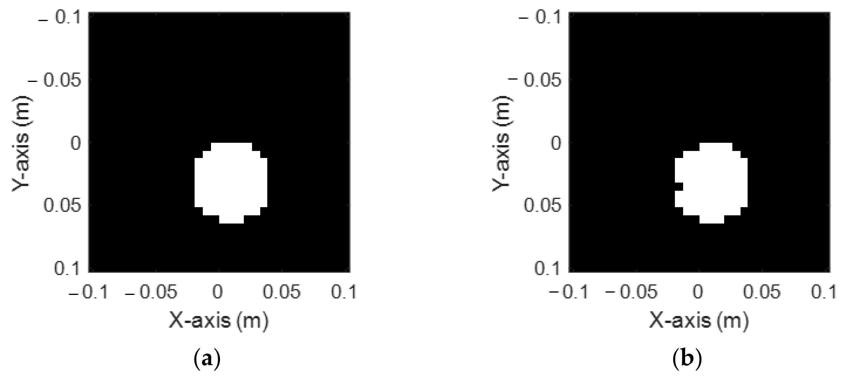
We reconstruct the images by using DCNN. As much as 5% noise is added to the scattered field to take care of the interference of external factors that may be encountered in reality and input the scattered field information into DCNN for training. Figure 4a,b shows the ground truth circular shape and the reconstructed shape by DCNN, respectively. It is seen that the reconstructed shape has a slight depression in the left half and a slight bulge in the upper half of the shape. In general, the reconstructed result is quite good. The RMSE and SSIM are 2.95% and 95.91%, respectively, as listed in

Table 1. RMSE and SSIM reconstructed images for case 1 to case 6.

	Method	RMSE	SSIM
Example
Case 1		2.95%	95.91%
Case 2		3.11%	94.18%
Case 3		17.81%	80.01%
Case 4		15.10%	83.82%
Case 5		14.14%	89.27%
Case 6		15.24%	86.73%

.

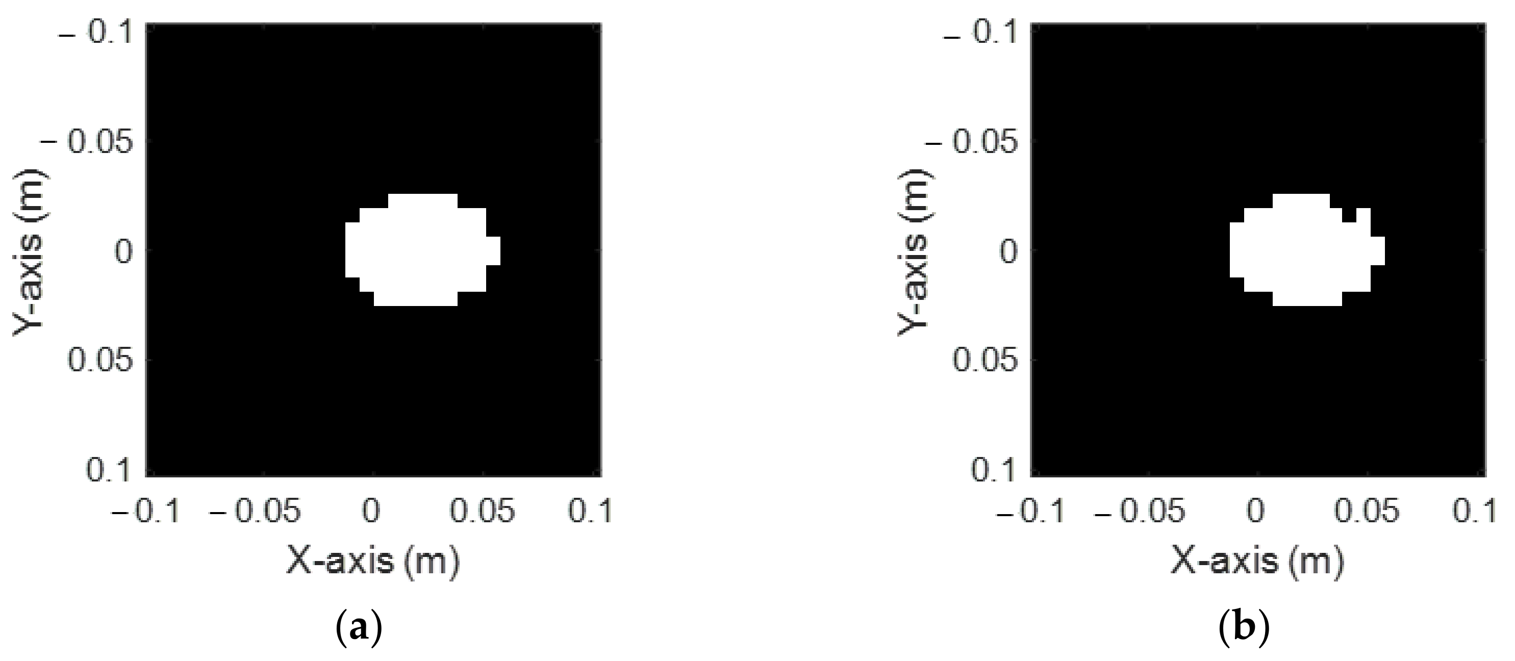
Figure 5a,b shows the ground truth elliptical shape and the reconstructed shape by DCNN, respectively. It is seen that the reconstructed shape has a slight depression in the upper right half and slightly protrudes in the upper half of the reconstructed shape. Generally, the reconstructed result is also perfect. The RMSE and SSIM are 3.11% and 94.18%, respectively, as listed in Table 1.

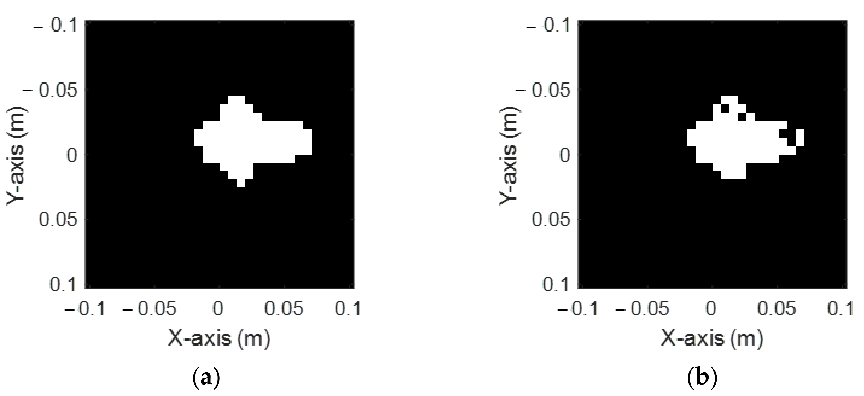
Figure 6a,b shows the ground truth arrow figure shape and the reconstructed shape by DCNN, respectively. It is seen that the reconstructed shape has some missing portions on the upper and right parts. In general, the reconstructed result is not perfect enough, though the size and position of the shape can still be recognized. The RMSE and SSIM are 17.81% and 80.01%, respectively, as listed in Table 1.

Figure 7a,b shows the ground truth peanut shape and the reconstructed shape by DCNN, respectively. It is seen that the reconstructed shape’s contour is slightly protruding. Generally, the reconstructed result is not good enough, though the size and position of the shape can still be recognized. The RMSE and SSIM are 15.10% and 83.82%, respectively, as listed in Table 1.

Figure 8a,b shows the ground truth four-petal shape and the reconstructed shape by DCNN, respectively. It is seen that the reconstructed shape’s petal appearance has little protrusions around it due to its relatively irregular shape, ensuring harder reconstruction. The RMSE and SSIM are 14.14% and 89.27%, respectively, as listed in Table 1.

Figure 9a,b shows the ground truth three-petal shape and the reconstructed shape by DCNN, respectively. It is seen that the reconstructed shape has a little protrusion on the upper part, but the size and position of the shape can still be recognized. The RMSE and SSIM are 15.24% and 86.73%, respectively, as listed in Table 1.

Above numerical results are given in Table 1. The average RMSE and SSIM of the entire testing set are 14.45% and 82.63%, respectively. Summarizing the above results, we can conclude that irregular conductor shapes, such as the arrow figure, peanut shape, and triple and quadruple petals, are more difficult to reconstruct than round and elliptical shapes.

Figure 10 highlights the effectiveness of the training process by plotting the loss results with respect to the number of epochs. In the beginning, the loss decreases very rapidly in the first 10 epochs. It decreases significantly between 10 and 20 epochs and decreases slowly between 20 and 80 epochs. It decreases very slowly between 80 and 140 epochs, and then slowly converges.

5. Conclusions

We have presented the two-dimensional inverse scattering reconstruction for perfect conductors buried in half-space via DCNN. We use the scattered field for the initial estimation. DCNN is employed in the frequency domain for reconstructing the accurate size and position of the shapes. According to our numerical simulation results, DCNN is highly reliable for reconstructing the perfect conductors. Based on our testing and training processes, the validation range of the DCNN could be determined. In addition, DCNN can recover better reconstruction results even when 5% noise is added to the scattered field. The method proposed here neither requires any regularization procedure such as direct methods or the traditional iterative method nor requires any initial guesses, which may be a big bottleneck for some algorithms, especially those that based on Newton iteration or backpropagation. Furthermore, the image can be reconstructed in just a few seconds once the training procedure is completed. It is also worth highlighting that the method is quite efficient, even under noise environments. Although simple images are being investigated in this paper, one future goal is to reconstruct images with complex dielectric distributions. Meanwhile, we will also try to innovate different neural network architectures simultaneously so that more accurate electromagnetic images can be reconstructed promptly.