Cascaded Convolutional Recurrent Neural Networks for EEG Emotion Recognition Based on Temporal–Frequency–Spatial Features

Featured Application

The proposed method can improve emotion recognition accuracy in human–computer interactions.

Abstract

Emotion recognition is a research area that spans multiple disciplines, including computational science, neuroscience, and cognitive psychology. The use of electroencephalogram (EEG) signals in emotion recognition is particularly promising due to their objective and nonartefactual nature. To effectively leverage the spatial information between electrodes, the temporal correlation of EEG sequences, and the various sub-bands of information corresponding to different emotions, we construct a 4D matrix comprising temporal–frequency–spatial features as the input to our proposed hybrid model. This model incorporates a residual network based on depthwise convolution (DC) and pointwise convolution (PC), which not only extracts the spatial–frequency information in the input signal, but also reduces the training parameters. To further improve performance, we apply frequency channel attention networks (FcaNet) to distribute weights to different channel features. Finally, we use a bidirectional long short-term memory network (Bi-LSTM) to learn the temporal information in the sequence in both directions. To highlight the temporal importance of the frame window in the sample, we choose the weighted sum of the hidden layer states at all frame moments as the input to softmax. Our experimental results demonstrate that the proposed method achieves excellent recognition performance. We experimentally validated all proposed methods on the DEAP dataset, which has authoritative status in the EEG emotion recognition domain. The average accuracy achieved was 97.84% for the four binary classifications of valence, arousal, dominance, and liking and 88.46% for the four classifications of high and low valence–arousal recognition.

1. Introduction

Emotion represents a complex psychological construct that encompasses an individual’s affective, cognitive, and behavioural responses to external stimuli, accompanied by corresponding physiological reactions [1]. In the modern era of intelligent technology, people’s daily lives are becoming increasingly intertwined with these advanced systems, underscoring the growing importance of accurate emotion recognition in human–computer interaction. Studies in neurological physiology [2] and social psychology [3] have revealed a strong correlation between EEG signals and numerous cognitive processes, including emotional responses, and can objectively reflect the real emotions of subjects, establishing EEG-based emotion recognition as a cutting-edge research area in cognitive science [4].

Owing to the nonlinear, unsmooth, low signal-to-noise ratio (SNR) and multichannel correlation characteristics of EEG data, which are inherently complex chaotic data, there are numerous data processing methods available in the research field [5], but the extraction of features that are highly relevant to emotions and the selection of a suitable classification model remain two obstacles for researchers. EEG signals have been demonstrated to contain emotion-related feature components in three dimensions: temporal, frequency, and spatial. Unfortunately, most of the literature considers only one or two of these three dimensions and performs pattern recognition by simple combinations, completely ignoring spatial information interactions across channels, prior knowledge across frequency bands, and information complementarity between different features. This not only fails to improve model accuracy, but also leads to feature redundancy and increased complexity. Therefore, it is important to improve emotion recognition accuracy by integrating information from different domains and adaptively capturing important temporal, frequency, and spatial features in subsequent classification models.

Recently, deep learning, the successor to machine learning, has made significant contributions to various fields, including computer vision (CV) and natural language processing (NLP). A wide range of deep models have been developed and have shown impressive results. The application of these models has also had a significant impact on EEG emotion recognition, including the use of autoencoders (AEs), graph convolutional neural networks (GCNs), transformers, and other related techniques. Although these approaches have yielded promising outcomes, challenges remain that need to be addressed. Specifically, how to construct a network that is suitable for EEG signal feature extraction represents a crucial issue that must be addressed.

Regarding the aforementioned challenges, a cascade network based on multidimensional features is proposed, which presents three main contributions:

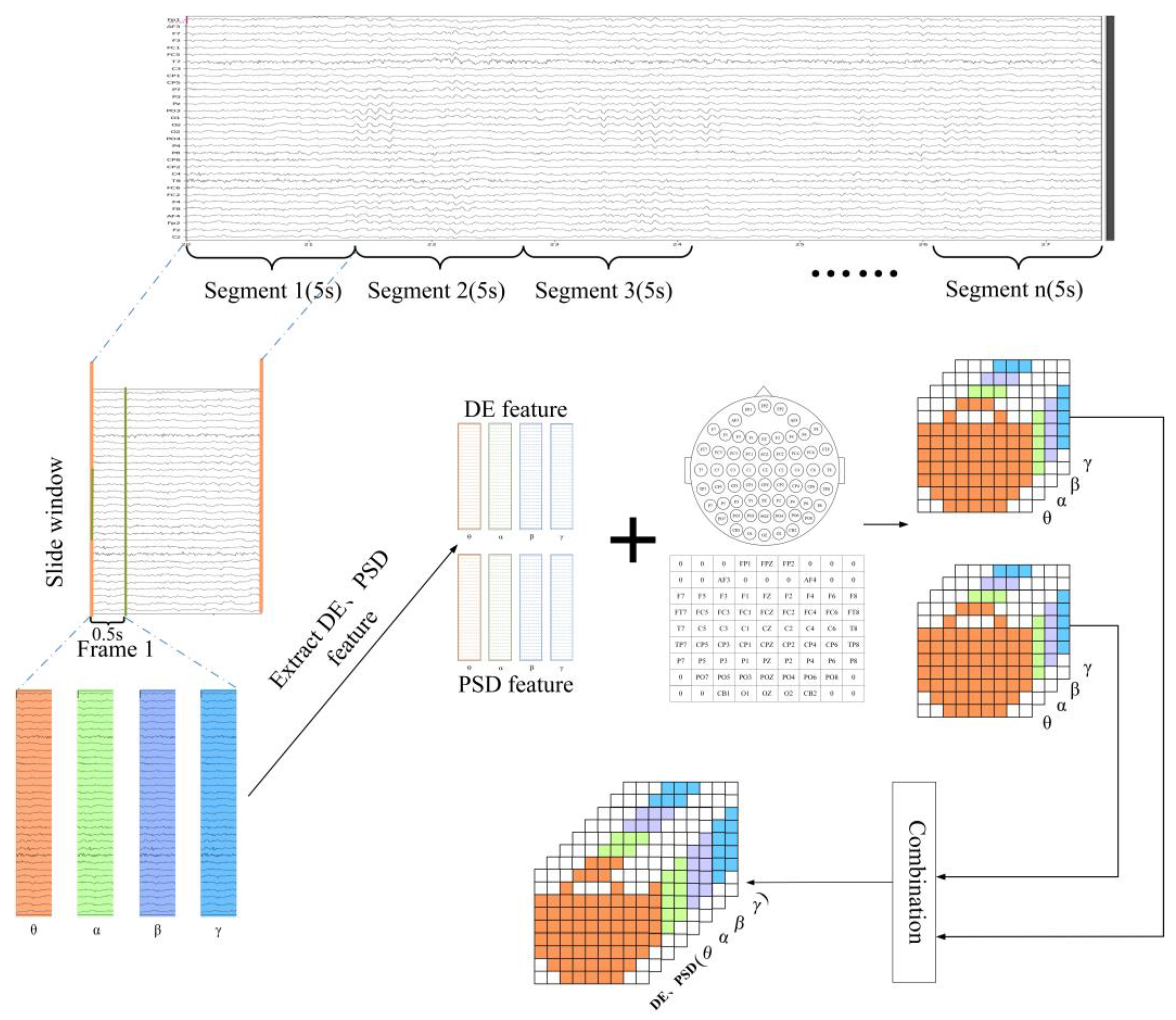
• EEG data are converted into a 4D matrix structure consisting of multiple frames, which contain information in three dimensions: temporal, frequency, and spatial, and can effectively represent the neural features of different emotions.
• In this paper, a novel attention module FcaNet is introduced. FcaNet redistributes the weights of different channels to obtain high-quality discrimination. FcaNet is found to be superior to traditional channel attention squeeze-and-excitation networks (SENet) while incurring no significant computational cost.
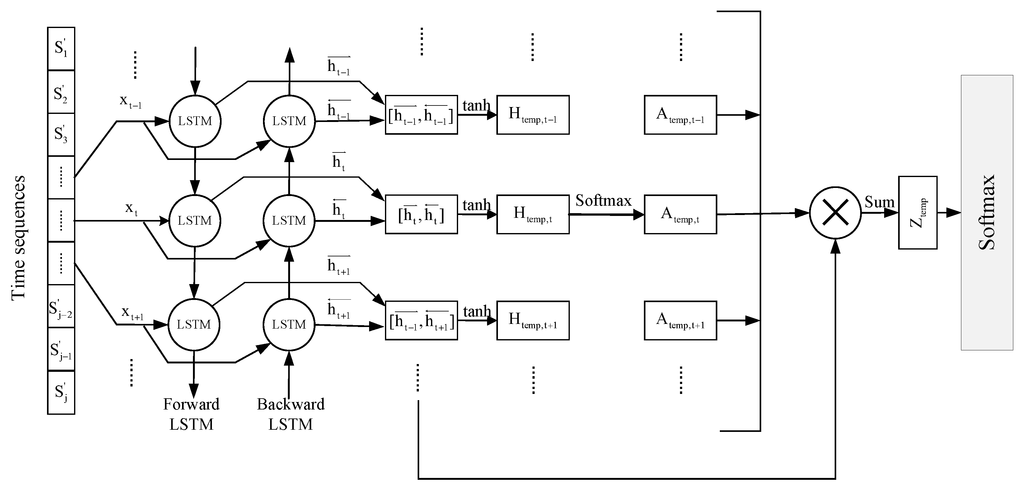
• To satisfy the real-time demands of the emotion recognition system, a residual network is devised, which comprises DC and PC to decrease the computational burden while utilizing the attributes of depth-separable convolution to segregate the spatial and channel mixing dimensions. Furthermore, the existence of a residual structure prevents overfitting. Ultimately, Bi-LSTM is employed to understand the temporal interdependence among different frames in the sample. The hidden layer states at each frame moment are allocated weights and then summed to serve as the input to softmax.

The experimental results show that the designed model achieves advanced performance on the DEAP dataset. The rest of the article is arranged as follows: Section 2: Related Work, Section 3: Methods, Section 4: Materials and Experimental Results, and Section 5: Conclusions.

2. Related Work

In the realm of emotion recognition, machine learning has traditionally been a popular approach for simple classification tasks [6]. Some prominent algorithms, including support vector machine (SVM), decision trees (DT), and k-nearest neighbour (KNN), have been successfully utilized in this field. Zubair [7] used the discrete wavelet transform (DWT) to extract temporal–frequency information and applied the maximum relevancy and minimum redundancy algorithm (mRMR) to select the most relevant features. In the literature [8,9], wavelet transform (WT) was applied for sub-band EEG signal decomposition, and the processed smooth feature information was then fed into SVM for classification. This method demonstrated promising improvement in accuracy for EEG emotion-state recognition in machine learning. However, machine learning techniques still face significant limitations when processing nonlinear and indistinguishable data, which restrict their capability for more complex classification tasks.

With the advent of deep learning, the machine learning limitations are gradually being overcome, and deep learning techniques are successfully moving in the direction of EEG emotions. Typically, deep-learning-based approaches focus on feature extraction from three dimensions: temporal, frequency, and spatial. For instance, in terms of the temporal information of EEG signals, Xing [10] proposed a framework combining a stacked autoencoder (SAE) and long short-term memory neural networks (LSTM). SAE is employed to simulate the mixing process in EEG and to separate the source signals. Then, the source signals are framed, and frequency features are extracted and combined into chained data, followed by discriminative classification using LSTM. Ma [11] designed the multimodal residual LSTM (MMResLSTM) network, using different LSTM layers to learn the temporal characteristics of different physiological signals and share parameters to achieve the information interaction of different modal data. References in the literature [12,13,14] introduced a temporal learning architecture that employs a 1D convolutional neural network (CNN) to extract temporal information from multichannel chained data.

Studies in neuroscience and psychology have proven that the $\mathrm{\delta }$-band (1–4 Hz), $\mathrm{\theta }$-band (4–8 Hz), $\mathrm{\alpha }$-band (8–13 Hz), $\mathrm{\beta }$-band (13–30 Hz), and $\mathrm{\gamma }$-band (30–50 Hz) of EEG [15] are associated with human emotions. Therefore, during the frequency domain feature extraction process, EEG signals are typically mapped onto these five frequency bands, and sub-band features are extracted. Zheng [16] extracted EEG signal differential entropy (DE) features on a sub-band and performed emotion recognition on a deep belief network (DBN). Zhang [17] extracted DE, power spectral density (PSD), differential asymmetry (DASM), and rational asymmetry (RASM) in four representative EEG datasets and trained them for classification by the proposed dynamic graph convolutional neural network (DGCNN). The results showed that the DE and PSD features could convey the most discriminative information.

Researchers have been interested in exploring physical models between electrode positions to characterize spatial features in EEG signals. Hwang [18] proposed a method to generate an image by performing a polar coordinate projection of the channel DE features and using different interpolation methods to fill the blank space after the projection, thus proving that the spatial topology based on electrode arrangement is effective. Song [19] utilized graph theoretic ideas to model multichannel EEG signals and used DGCNN to explore the depth spatial information of neighbouring channels. Other studies [20,21,22,23] constructed a connectivity matrix containing structural information of the brain to express features in different ways and then input the rearranged EEG signals into an end-to-end CNN model.

The researchers have also considered various feature information combinations. References from the literature [23,24] extracted the DE features of the four EEG signal sub-bands, which were mapped into a 3D matrix based on the electrode distribution to retain its channel information. Finally, the spatial–frequency information was extracted by different 2D convolutions. Researchers in [25,26,27,28] introduced a combined CNN and LSTM model that learns spatial–frequency and temporal features, respectively, from the input signal. Experimental findings reveal that the accuracy of combined multidimensional feature information surpasses that of a single dimension.

There exists a broad range of feature extraction methods; however, fully exploiting key features remains a significant challenge. Introducing an attention mechanism has greatly enhanced the capabilities of various classification models. Researchers in EEG emotion recognition have noted that attentional mechanisms can selectively focus on brain regions associated with emotional stimulation and have begun to explore their application to EEG emotion recognition to improve performance. Zhang [29] introduced band attention and temporal attention in a hybrid deep learning model to adaptively assign weights for different frequency bands and times, respectively. In [22,30], researchers constructed 3D data containing temporal–frequency information, introduced the channel attention module SENet to assign weights to frequency bands and channels, and obtained advanced results.

3. Methods

In this section, data preprocessing and the three components of the proposed model are explained in detail. A complete overview of the model framework is shown in Figure 1.

3.1. Data Preprocessing

In the original data acquisition, a few seconds of the steady state of the subject before the emotional stimulus is recorded. Most studies choose to remove this part of the data directly when recognizing the task and consider only the EEG signal in the stimulated state. Studies [25,30,31] demonstrated that preprocessing through the baseline signal is effective for improving experimental robustness. The difference between the signal of the subject under the emotional stimulus and the baseline signal was calculated as an indication that the segment’s emotional state data could yield the expected results. Assume that the dataset is sampled at a frequency of S. Consider the entire baseline clip ${\mathrm{X}}_{\mathrm{b}\mathrm{a}s\mathrm{e}}\in {\mathrm{R}}^{\mathrm{M}\mathrm{x}{\mathrm{N}}_1}$, where M is the number of electrodes: 32; and ${\mathrm{N}}_1$ is the sum of the sampling points for the entire baseline clip. First, ${\mathrm{X}}_{\mathrm{b}\mathrm{a}\mathrm{s}\mathrm{e}}$ is uniformly divided into 1 s periods to obtain $\{{\mathrm{X}}_{\mathrm{base}}^1,{\mathrm{X}}_{\mathrm{base}}^2,\dots ,{\mathrm{X}}_{\mathrm{base}}^{\mathrm{O}}\}$, ${\mathrm{X}}_{\mathrm{base}}^{\mathrm{i}}\in {\mathrm{R}}^{\mathrm{M}\mathrm{xS}}$$(\mathrm{i}=1,2,\dots ,\mathrm{O})$ denoting the i-th baseline segment, $\mathrm{O}=\frac{{\mathrm{N}}_1}{\mathrm{S}}$. Then, the average value ${\overline{\mathrm{X}}}_{\mathrm{b}\mathrm{a}\mathrm{s}\mathrm{e}}\in {\mathrm{R}}^{\mathrm{M}\mathrm{x}\mathrm{S}}$ of ${\mathrm{X}}_{\mathrm{b}\mathrm{a}\mathrm{s}\mathrm{e}}$ is calculated as follows:

$${\overline{\mathrm{X}}}_{\mathrm{b}\mathrm{a}\mathrm{s}\mathrm{e}}=\frac{{\displaystyle \sum _{\mathrm{i}=1}^{\mathrm{O}}{\mathrm{X}}_{\mathrm{base}}^{\mathrm{i}}}}{\mathrm{O}}$$

(1)

${\mathrm{X}}_{\mathrm{t}\mathrm{r}\mathrm{i}\mathrm{a}\mathrm{l}}\in {\mathrm{R}}^{\mathrm{M}\mathrm{x}{\mathrm{N}}_2}$ denotes the experimental EEG signal in the emotional stimulation condition, and ${\mathrm{N}}_2$ denotes the total number of sampling points of the experimental EEG signal. As in the above method, the experimental data were split into Q segments according to the length criterion of ${\overline{\mathrm{X}}}_{\mathrm{b}\mathrm{a}\mathrm{s}\mathrm{e}}$ to obtain $\{{\mathrm{X}}_{\mathrm{t}\mathrm{r}\mathrm{i}\mathrm{a}\mathrm{l}}^1,{\mathrm{X}}_{\mathrm{t}\mathrm{r}\mathrm{i}\mathrm{a}\mathrm{l}}^2,\dots ,{\mathrm{X}}_{\mathrm{t}\mathrm{r}\mathrm{i}\mathrm{a}\mathrm{l}}^{\mathrm{Q}}\}$, where ${\mathrm{X}}_{\mathrm{t}\mathrm{r}\mathrm{i}\mathrm{a}\mathrm{l}}^{\mathrm{i}}\in {\mathrm{R}}^{\mathrm{M}\mathrm{xS}}$ $(\mathrm{i}=1,2,\dots ,\mathrm{Q})$ denotes the i-th experimental segment, and $\mathrm{Q}=\frac{{\mathrm{N}}_2}{\mathrm{S}}$. Finally, the baseline removal data were obtained by subtracting the baseline mean ${\overline{\mathrm{X}}}_{\mathrm{b}\mathrm{a}\mathrm{s}\mathrm{e}}$ from each segment of the experimental data using the following equation:

$${\mathrm{X}}_{\mathrm{t}\mathrm{r}\mathrm{i}\mathrm{a}\mathrm{l}.\mathrm{r}\mathrm{m}\mathrm{o}\mathrm{v}}^{\mathrm{i}}={\mathrm{X}}_{\mathrm{t}\mathrm{r}\mathrm{i}\mathrm{a}\mathrm{l}}^{\mathrm{i}}-{\overline{\mathrm{X}}}_{\mathrm{b}\mathrm{a}\mathrm{s}\mathrm{e}},{\mathrm{X}}_{\mathrm{t}\mathrm{r}\mathrm{i}\mathrm{a}\mathrm{l}.\mathrm{r}\mathrm{m}\mathrm{o}\mathrm{v}}^{\mathrm{i}}\in {\mathrm{R}}^{\mathrm{M}\times \mathrm{S}}$$

(2)

where ${\mathrm{X}}_{\mathrm{t}\mathrm{r}\mathrm{i}\mathrm{a}\mathrm{l}.\mathrm{r}\mathrm{m}\mathrm{o}\mathrm{v}}^{\mathrm{i}}$$(\mathrm{i}=1,2,\dots ,\mathrm{Q})$ represents the contrast data from ${\mathrm{X}}_{\mathrm{t}\mathrm{r}\mathrm{i}\mathrm{a}\mathrm{l}}^{\mathrm{i}}$ and ${\overline{\mathrm{X}}}_{\mathrm{b}\mathrm{a}\mathrm{s}\mathrm{e}}$. Finally, the Q segment removed the baseline data to patch the complete data ${\mathrm{X}}_{\mathrm{t}\mathrm{r}\mathrm{i}\mathrm{a}\mathrm{l}.\mathrm{r}\mathrm{m}\mathrm{o}\mathrm{v}}=\{{\mathrm{X}}_{\mathrm{t}\mathrm{r}\mathrm{i}\mathrm{a}\mathrm{l}.\mathrm{r}\mathrm{m}\mathrm{o}\mathrm{v}}^1,{\mathrm{X}}_{\mathrm{t}\mathrm{r}\mathrm{i}\mathrm{a}\mathrm{l}.\mathrm{r}\mathrm{m}\mathrm{o}\mathrm{v}}^2,\dots ,{\mathrm{X}}_{\mathrm{t}\mathrm{r}\mathrm{i}\mathrm{a}\mathrm{l}.\mathrm{r}\mathrm{m}\mathrm{o}\mathrm{v}}^{\mathrm{Q}}\}$, ${\mathrm{X}}_{\mathrm{t}\mathrm{r}\mathrm{i}\mathrm{a}\mathrm{l}.\mathrm{r}\mathrm{m}\mathrm{o}\mathrm{v}}\in {\mathrm{R}}^{\mathrm{M}\mathrm{x}{\mathrm{N}}_2}$, which was performed on ${\mathrm{X}}_{\mathrm{t}\mathrm{r}\mathrm{i}\mathrm{a}\mathrm{l}.\mathrm{r}\mathrm{m}\mathrm{o}\mathrm{v}}$ in the subsequent feature extraction.

3.2. Multiband Four-Dimensional Feature Construction

In this section, the process of forming a 4D matrix based on the temporal–frequency–spatial is explained in detail, as shown in Figure 2.

Since the integration of temporal and frequency band information of all available channels requires a three-dimensional spatial representation, this requires the consideration of a matrix of filtered signals obtained from all channels. Take the DEAP dataset as an example, which includes a total of 1280 sample data points (32 subjects × 40 experiments). For the problem that a small quantity of data can cause overfitting when the network layers are deep, we reduce this effect by increasing the number of samples. Specifically, for the signal ${\mathrm{X}}_{\mathrm{t}\mathrm{r}\mathrm{i}\mathrm{a}\mathrm{l}.\mathrm{r}\mathrm{m}\mathrm{o}\mathrm{v}}\in {\mathrm{R}}^{\mathrm{M}\times {\mathrm{N}}_2}$ after baseline removal, a nonoverlapping windowing process with a time duration of u seconds (design in this paper with u = 5 s) is performed to obtain the divided data $\{{\mathrm{X}}_{\mathrm{S}}^1,{\mathrm{X}}_{\mathrm{S}}^2,\dots ,{\mathrm{X}}_{\mathrm{S}}^{\mathrm{n}}\}$, where the ith window segment ${\mathrm{X}}_{\mathrm{S}}^{\mathrm{i}}=\{{\mathrm{x}}_1,{\mathrm{x}}_2,\dots ,{\mathrm{x}}_{\mathrm{M}}\}\in {\mathrm{R}}^{\mathrm{M}\times \mathrm{R}}(\mathrm{i}=1,2,\dots ,\mathrm{n})$, ${\mathrm{x}}_{\mathrm{c}}\in {\mathrm{R}}^{\mathrm{R}}(\mathrm{c}=1,2,\dots ,\mathrm{M})$ denotes data from the c-th electrode channel in ${\mathrm{X}}_{\mathrm{S}}^{\mathrm{i}}$, and R is the sampling frequency of the whole window segment.

Different frequency band data in EEG reflect different emotional information, as detailed in

Table 1. Emotional states correspond to different frequency band information.

Frequency Band	Frequency Range	Brain States	Awareness
$\mathrm{\delta }$	1–4	Extreme fatigue and deep sleep states	Sleep mode
$\mathrm{\theta }$	4–8	Light sleep, frustrated state	Low
$\mathrm{\alpha }$	8–13	Awake, quiet, and eyes closed state	Medium
$\mathrm{\beta }$	13–30	Active thinking, mental tension, anxiety, concentration state	High
$\mathrm{\gamma }$	30–50	Multimodal sensory stimulation, mentally active state	High

[32]. While conducting directional research, the linear data phase is commonly required to be high. A finite impulse response filter (FIR) can obtain a rigorous linear phase with high stationarity and low interference power caused by operational errors. Therefore, we use FIR to have a sub-band division for each window segment ${\mathrm{X}}_{\mathrm{S}}^{\mathrm{i}}$. Qu [25] experimentally compared the EEG emotion recognition results under different band combinations and found that band combinations of $\mathrm{\alpha }$, $\mathrm{\beta }$, and $\mathrm{\gamma }$ had the highest accuracy in task recognition. In addition, Frantzidis [33] remarked that the $\mathrm{\theta }$-band features are closely correlated with arousal. Therefore, in this paper, the four bands $\mathrm{\theta },\mathrm{\alpha },\mathrm{\beta },\mathrm{\gamma }$ were chosen to study the emotional state features of EEG signals. Through the FIR filter, each window segment was decomposed into ${\mathrm{X}}_{\mathrm{S}}^{\mathrm{i}}=\left\{\right\{{\mathrm{f}}_1^{\mathrm{\theta }},{\mathrm{f}}_1^{\mathrm{\alpha }},{\mathrm{f}}_1^{\mathrm{\beta }},{\mathrm{f}}_1^{\mathrm{\gamma }}\},\dots ,\{{\mathrm{f}}_{\mathrm{M}}^{\mathrm{\theta }},{\mathrm{f}}_{\mathrm{M}}^{\mathrm{\alpha }},{\mathrm{f}}_{\mathrm{M}}^{\mathrm{\beta }},{\mathrm{f}}_{\mathrm{M}}^{\mathrm{\gamma }}\left\}\right\}$$(\mathrm{i}=1,2,\dots ,\mathrm{n})$. The specific realization formula is as follows:

$$\mathrm{h}(\mathrm{n})={\mathrm{h}}_{\mathrm{d}}(\mathrm{n})\cdot \mathrm{w}(\mathrm{n})=\frac{\sin [(\mathrm{M}-\mathrm{\tau })\cdot {\mathrm{W}}_{\mathrm{h}}]-\sin [(\mathrm{M}-\mathrm{\tau })\cdot {\mathrm{W}}_{\mathrm{l}}]}{\mathrm{\pi }\cdot (\mathrm{m}-\mathrm{\tau })}\cdot \mathrm{w}(\mathrm{n})$$

(3)

$${\mathrm{H}}_{\mathrm{d}}({\mathrm{e}}^{\mathrm{j}\mathrm{w}})={\displaystyle \sum _{\mathrm{n}=-\infty }^{\mathrm{n}=+\infty }{\mathrm{h}}_{\mathrm{d}}(\mathrm{n})}{\mathrm{e}}^{-\mathrm{j}\mathrm{w}\mathrm{n}}$$

(4)

$$\mathrm{H}(\mathrm{w})=|\mathrm{H}({\mathrm{e}}^{\mathrm{j}\mathrm{w}})|=|\frac{1}{2\mathrm{\pi }}{\displaystyle \underset{-\mathrm{\pi }}{\overset{\mathrm{\pi }}{\int }}({\mathrm{H}}_{\mathrm{d}}({\mathrm{e}}^{\mathrm{j}\mathrm{\theta }})}{\mathrm{e}}^{-\mathrm{j}\mathrm{\theta }\mathrm{M}/2})\mathrm{W}({\mathrm{e}}^{\mathrm{j}\mathrm{w}})\mathrm{d}\mathrm{\theta }|$$

(5)

where $\mathrm{h}(\mathrm{n})$ is the filter coefficient, ${\mathrm{H}}_{\mathrm{d}}({\mathrm{e}}^{\mathrm{j}\mathrm{w}})$ is the corresponding frequency response, $\mathrm{H}(\mathrm{w})$ is the amplitude–frequency response function, ${\mathrm{h}}_{\mathrm{d}}(\mathrm{n})$ is the unit impulse response, $\mathrm{w}(\mathrm{n})$ is the window function, ${\mathrm{W}}_{\mathrm{h}}$ and ${\mathrm{W}}_{\mathrm{l}}$ are the cut-off frequencies of the bandpass filter, $\mathrm{\tau }=\frac{\mathrm{M}-1}{2}$, and M is the number of filter steps.

Treating all channel data of a single frequency band as a whole, such that ${\mathrm{X}}_{\mathrm{S}}^{\mathrm{i}}$ is transformed into $\{{\mathrm{p}}_{\mathrm{i}}^{\mathrm{\theta }},{\mathrm{p}}_{\mathrm{i}}^{\mathrm{\alpha }},{\mathrm{p}}_{\mathrm{i}}^{\mathrm{\beta }},{\mathrm{p}}_{\mathrm{i}}^{\mathrm{\gamma }}\}$, where $\mathrm{p}=\{{\mathrm{p}}_1,{\mathrm{p}}_2,\dots ,{\mathrm{p}}_{\mathrm{M}}\}$ denotes all channel data of a single frequency band, the arrangement order is shown in Figure 3.

After data enhancement, our focus shifts to emotion recognition at the segmentation level, and considering that human emotion changes are temporally dynamic, the window segmented signal ${\mathrm{X}}_{\mathrm{S}}^{\mathrm{i}}$ is segmented into equal-length frames of 0.5 s. Using 0.5 s data per channel as the vector components that constitute a single frame window, ${\mathrm{X}}_{\mathrm{S}}^{\mathrm{i}}$ will be converted into a sequence containing 2u frame vectors, ${\mathrm{X}}_{\mathrm{S}}^{\mathrm{i}}=\left\{\right\{{\mathrm{p}}_{\mathrm{i}}^{1\mathrm{\theta }},{\mathrm{p}}_{\mathrm{i}}^{1\mathrm{\alpha }},{\mathrm{p}}_{\mathrm{i}}^{1\mathrm{\beta }},{\mathrm{p}}_{\mathrm{i}}^{1\mathrm{\gamma }}\},\dots ,\{{\mathrm{p}}_{\mathrm{i}}^{\mathrm{j}\mathrm{\theta }},{\mathrm{p}}_{\mathrm{i}}^{\mathrm{j}\mathrm{\alpha }},{\mathrm{p}}_{\mathrm{i}}^{\mathrm{j}\mathrm{\beta }},{\mathrm{p}}_{\mathrm{i}}^{\mathrm{j}\mathrm{\gamma }}\left\}\right\}$ $(\mathrm{i}=1,2,\dots ,\mathrm{n}.\mathrm{j}=1,2,\dots ,2\mathrm{u})$. Considering the information complementarity between different features, the DE and PSD features of all channels within each frame window are extracted in this paper [16].

DE is a derivative of Shannon’s concept of information entropy over a continuous probability distribution, which is a good method to describe internal EEG information. A specific length of EEG that approximately obeys the Gauss distribution $\mathrm{N}(\mathrm{\mu },{\mathrm{\sigma }}_{\mathrm{i}}^2)$ is calculated as:

$$\mathrm{D}\mathrm{E}=-{\displaystyle {\int }_{-\infty }^{+\infty }\frac{1}{\sqrt{2\mathrm{\pi }{\mathrm{\sigma }}_{\mathrm{i}}^2}}}{\mathrm{e}}^{-\frac{{(\mathrm{x}-\mathrm{\mu })}^2}{2{\mathrm{\sigma }}_{\mathrm{i}}^2}}\log (\frac{1}{\sqrt{2\mathrm{\pi }{\mathrm{\sigma }}_{\mathrm{i}}^2}}{\mathrm{e}}^{-\frac{{(\mathrm{x}-\mathrm{\mu })}^2}{2{\mathrm{\sigma }}_{\mathrm{i}}^2}})\mathrm{d}\mathrm{x}=\frac{1}{2}\log (2\mathrm{\pi }\mathrm{e}{\mathrm{\sigma }}_{\mathrm{i}}^2)$$

(6)

where $\mathrm{\sigma }$ is the variance in the sequence signal.

PSD is a physical quantity that characterizes the relationship between the power energy of a signal and its frequency and is often used to study random vibration signals, which can describe the activation level and emotional complexity of EEG signals. It is calculated as:

$$\mathrm{P}(\mathrm{w})=\frac{1}{\mathrm{M}\mathrm{U}}{\left|{\displaystyle \sum _{\mathrm{n}=0}^{\mathrm{M}-1}{\mathrm{x}}_{\mathrm{N}}^{\mathrm{i}}(\mathrm{n})\mathrm{d}(\mathrm{n}){\mathrm{e}}^{-\mathrm{j}\mathrm{w}\mathrm{n}}}\right|}^2$$

(7)

where ${\mathrm{x}}_{\mathrm{N}}^{\mathrm{i}}(\mathrm{n})$ is the sampled data in segment i, $\mathrm{d}(\mathrm{n})$ is the selected window function, M is the length of each segment, and U is the normalization factor.

The final two sets of features obtained both include a two-dimensional vector sequence of four frequency bands, where the frame vectors ${\mathrm{f}}_{\mathrm{i}}^{\mathrm{j}\mathrm{\gamma }}$ and ${\mathrm{g}}_{\mathrm{i}}^{\mathrm{j}\mathrm{\gamma }}$ retain the same arrangement as ${\mathrm{p}}_{\mathrm{i}}^{\mathrm{j}\mathrm{\gamma }}$. It can be described as:

$${\mathrm{F}}_{\mathrm{P}\mathrm{S}\mathrm{D}}=\mathrm{PSD}({\mathrm{X}}_{\mathrm{S}}^{\mathrm{i}})=\left\{\right\{{\mathrm{f}}_{\mathrm{i}}^{1\mathrm{\theta }},{\mathrm{f}}_{\mathrm{i}}^{1\mathrm{\alpha }},{\mathrm{f}}_{\mathrm{i}}^{1\mathrm{\beta }},{\mathrm{f}}_{\mathrm{i}}^{1\mathrm{\gamma }}\},\dots ,\{{\mathrm{f}}_{\mathrm{i}}^{\mathrm{j}\mathrm{\theta }},{\mathrm{f}}_{\mathrm{i}}^{\mathrm{j}\mathrm{\alpha }},{\mathrm{f}}_{\mathrm{i}}^{\mathrm{j}\mathrm{\beta }},{\mathrm{f}}_{\mathrm{i}}^{\mathrm{j}\mathrm{\gamma }}\left\}\right\}$$

(8)

$${\mathrm{F}}_{\mathrm{D}\mathrm{E}}=\mathrm{DE}({\mathrm{X}}_{\mathrm{S}}^{\mathrm{i}})=\left\{\right\{{\mathrm{g}}_{\mathrm{i}}^{1\mathrm{\theta }},{\mathrm{g}}_{\mathrm{i}}^{1\mathrm{\alpha }},{\mathrm{g}}_{\mathrm{i}}^{1\mathrm{\beta }},{\mathrm{g}}_{\mathrm{i}}^{1\mathrm{\gamma }}\},\dots ,\{{\mathrm{g}}_{\mathrm{i}}^{\mathrm{j}\mathrm{\theta }},{\mathrm{g}}_{\mathrm{i}}^{\mathrm{j}\mathrm{\alpha }},{\mathrm{g}}_{\mathrm{i}}^{\mathrm{j}\mathrm{\beta }},{\mathrm{g}}_{\mathrm{i}}^{\mathrm{j}\mathrm{\gamma }}\left\}\right\}$$

(9)

Nevertheless, frequency features can never fully characterize all the feature components of the entire signal. The EEG is obtained from electrodes placed in different regions for acquisition, and the positional relationships between these electrodes contain information about the spatial structure associated with emotions. Therefore, in this paper, a single frequency band frame vector is mapped into a two-dimensional matrix using spatial mapping. References [34,35,36] proposed the sparse transform, compact transform, and sensitive transform methods, respectively. The sparse transformation matrix is 19 × 19, which undoubtedly requires many computations [34]. The compact matrix of Shen [35] reduces the size to 8 × 9, which drastically reduces the computational effort, and the adjacent electrodes in the matrix are more strongly connected, but it is not sensitive to spatial information and does not work well experimentally. Therefore, here, we use the sensitive transformation method of Xu [36] to map it to 9 × 9 data. Compared with the first two methods, the connection relationship between electrode points is more in line with the “10/20” system while considering the computational effort. These three specific mapping methods are shown in Figure 4. Each frame vector ${\mathrm{f}}_{\mathrm{i}}^{\mathrm{j}\mathrm{\gamma }}$ of a single frequency band is further converted into a two-dimensional matrix. SEED and DEAP each contain 62 and 32 electrode channels, so here, 62 channels are used to map the electrode positions, the corresponding DE and PSD values are filled for the elements with position mapping, and the remaining positions are replaced by 0. In this way, the window segments transform into a two-dimensional matrix sequence from the perspective of a single frequency band. Taking the $\mathrm{\theta }$-band as an example, ${\mathrm{S}}^{\mathrm{\theta }}=\{{\mathrm{S}}_1^{\mathrm{\theta }},{\mathrm{S}}_2^{\mathrm{\theta }},\dots ,{\mathrm{S}}_{\mathrm{j}}^{\mathrm{\theta }}\}\in {\mathrm{R}}^{9\times 9\times 2\mathrm{u}}$$(\mathrm{j}=1,2,\dots ,2\mathrm{u})$, it is extended into 3 dimensions in dimensionality. The four-dimensional data of a single feature in the whole window fragment are obtained by fusing the four frequency bands. Taking the DE feature of the window fragment as an example, $\mathrm{S}=\{{\mathrm{S}}_{(\mathrm{D}\mathrm{E})1},{\mathrm{S}}_{(\mathrm{D}\mathrm{E})2},\dots ,{\mathrm{S}}_{(\mathrm{D}\mathrm{E})\mathrm{j}}\}\in {\mathrm{R}}^{9\times 9\times 8\times 2\mathrm{u}}$, considering the problem of information complementarity between different features, we place the same frequency band data of DE and PSD features together to construct the final four-dimensional data $\mathrm{S}=\{{\mathrm{S}}_1,{\mathrm{S}}_2,\dots ,{\mathrm{S}}_{\mathrm{j}}\}\in {\mathrm{R}}^{9\times 9\times 8\times 2\mathrm{u}}$.

After obtaining the mapping matrix of all frame window feature data, Equation (10) is used to normalize the data to a distribution with a mean of 0 and a variance of 1, attempting to avoid poles that may negatively affect the recognition results during gradient descent.

$${\mathrm{x}}_{\mathrm{s}\mathrm{c}\mathrm{a}\mathrm{l}\mathrm{e}}=\frac{(\mathrm{x}-{\mathrm{x}}_{\mathrm{m}\mathrm{e}\mathrm{a}\mathrm{n}})}{\mathrm{\sigma }}$$

(10)

where ${\mathrm{x}}_{\mathrm{m}\mathrm{e}\mathrm{a}\mathrm{n}}$ is the mean of the eigenvalue data, $\mathrm{\sigma }$ is the standard deviation of each set of features, $\mathrm{x}$ is the actual eigenvalue, and ${\mathrm{x}}_{\mathrm{s}\mathrm{c}\mathrm{a}\mathrm{l}\mathrm{e}}$ is the final normalized data.

3.3. Network Architecture

3.3.1. FcaNet

In this study, the aim is to obtain high-quality EEG feature information. To achieve this goal, we incorporated an attention module called FcaNet [37] into the backbone network, which is used to lower the weight of low-quality EEG information. FcaNet is a novel attention module based on SENet [38], which was initially used in target detection. Unlike the global average pooling (GAP) used in SENet to squeeze the feature map, FcaNet uses two-dimensional discrete cosine transformation (2D-DCT) for the same purpose. GAP corresponds only to the lowest frequency portion of the 2D-DCT, resulting in the loss of the remaining frequency portions in the channel. A comparison of SENet and FcaNet is shown in Figure 5.

Given an input X, it is divided into n parts along the channel dimension: $\left[{\mathrm{X}}^0,{\mathrm{X}}^1,{\mathrm{X}}^2,\dots ,{\mathrm{X}}^{\mathrm{n}-1}\right]$, where $\mathrm{i}\in \left\{0,1,2,\dots ,\mathrm{n}-1\right\}$, ${\mathrm{X}}^{\mathrm{i}}\in {\mathrm{R}}^{\mathrm{H}\times \mathrm{W}\times {\mathrm{C}}^{\prime }}$, ${\mathrm{C}}^{\prime }=\frac{\mathrm{C}}{\mathrm{n}}$. For each part, the corresponding 2D-DCT frequency portion is distributed, and the result of 2D-DCT is used as the compression result noted by the channel. The following equation shows 2D-DCT:

$$\mathrm{F}\mathrm{r}\mathrm{e}{\mathrm{q}}^{\mathrm{i}}=2\mathrm{D}\mathrm{D}\mathrm{C}{\mathrm{T}}^{{\mathrm{u}}_{\mathrm{i}},{\mathrm{v}}_{\mathrm{i}}}({\mathrm{X}}^{\mathrm{i}})={\displaystyle \sum _{\mathrm{h}=0}^{\mathrm{H}-1}{\displaystyle \sum _{\mathrm{w}=0}^{\mathrm{W}-1}{\mathrm{X}}_{:,\mathrm{h},\mathrm{w}}^{\mathrm{i}}{\mathrm{B}}_{\mathrm{h},\mathrm{w}}^{{\mathrm{u}}_{\mathrm{i}},{\mathrm{v}}_{\mathrm{i}}}}}$$

(11)

$${\mathrm{B}}_{\mathrm{h},\mathrm{w}}^{{\mathrm{u}}_{\mathrm{i}},{\mathrm{v}}_{\mathrm{i}}}=\cos (\frac{\mathrm{\pi }\mathrm{h}}{\mathrm{H}}({\mathrm{u}}_{\mathrm{i}}+\frac{1}{2}))\cos (\frac{\mathrm{\pi }\mathrm{w}}{\mathrm{W}}({\mathrm{v}}_{\mathrm{i}}+\frac{1}{2}))$$

(12)

$$\mathrm{s},\mathrm{t}.\mathrm{i}\in \{0,1,\dots ,\mathrm{n}-1\}$$

where H, W, and $({\mathrm{u}}_{\mathrm{i}},{\mathrm{v}}_{\mathrm{i}})$ are the height, width, and 2D index of ${\mathrm{X}}^{\mathrm{i}}$, respectively. The whole feature information compression vector can be represented by cascading as:

$$\mathrm{F}\mathrm{r}\mathrm{e}\mathrm{q}=\mathrm{c}\mathrm{o}\mathrm{m}\mathrm{p}\mathrm{r}\mathrm{e}\mathrm{s}\mathrm{s}(\mathrm{X})=\mathrm{c}\mathrm{a}\mathrm{t}([\mathrm{F}\mathrm{r}\mathrm{e}{\mathrm{q}}^0,\mathrm{F}\mathrm{r}\mathrm{e}{\mathrm{q}}^1,\dots ,\mathrm{F}\mathrm{r}\mathrm{e}{\mathrm{q}}^{\mathrm{n}-1}])$$

(13)

The complete FcaNet framework can be described as follows:

$$\mathrm{m}\mathrm{s}\_\mathrm{a}\mathrm{t}\mathrm{t}=\mathrm{s}\mathrm{i}\mathrm{g}\mathrm{m}\mathrm{o}\mathrm{i}\mathrm{d}(\mathrm{f}\mathrm{c}(\mathrm{F}\mathrm{r}\mathrm{e}\mathrm{q}))$$

(14)

3.3.2. Spatial–Frequency Feature Learning

Extracting spatial–frequency features is primarily accomplished through the use of the convolutional encoder and the attention module FcaNet discussed in Section 3.3.1, with the module structure illustrated in Figure 6.

Specifically, 2u frames ${\mathrm{S}}_{\mathrm{j}}$ in each segment are fed into the CNN module sequentially in time order, and the three-dimensional data structure of each frame is 9 × 9 × 8. To better retain information in the relatively small three-dimensional data structure, two convolutional layers are first implemented. The first layer employs a 1 × 1 convolution kernel with 64 kernels, and the second layer utilizes a 3 × 3 convolutional kernel with 128 kernels. These different convolutional kernels are utilized to extract deeper information from the three-dimensional data. Subsequently, the residual network is constructed using DC and PC. This combination reduces the number of training parameters while extracting internal features from expanded individual feature maps using DC and expressing cross-feature map relationships using PC. Moreover, the residual structure effectively avoids network degradation. ReLU is utilized as the activation function for each convolutional layer, and BatchNorm processing is performed. Padding operations are carried out for DC to maintain output size consistency for each layer of convolution. FcaNet assigns weights to different channel features to enhance model performance. The data are subjected to dimensionality reduction through the utilization of a 2 × 2 maximum pooling layer at the end of the cycle, followed by one-dimensional data transformation via flattened layer processing. Finally, each data frame is convolutionally encoded to obtain vector ${\mathrm{S}}_{\mathrm{j}}^{\prime }\in {\mathrm{R}}^{1152}$.

3.3.3. Temporal Feature Learning

Since emotion changes are temporally dynamic, changes between frames in four-dimensional data may hide emotion-related information. To explore the temporal correlation features in the whole window segment, we input the spatial–frequency features ${\mathrm{S}}^{\prime }=\{{\mathrm{S}}_1^{\prime },{\mathrm{S}}_2^{\prime },\dots ,{\mathrm{S}}_{\mathrm{j}}^{\prime }\}$ obtained after convolutional coding into the Bi-LSTM network in time order for coding.

LSTM solves the problem that its distant text information cannot be exploited and its close distance but not much semantic association is based on the traditional recurrent neural networks (RNN). It is a model for processing sequential signals that can mitigate the gradient disappearance that occurs with long sequence inputs in RNN. The computational equation of an LSTM cell is shown as:

$${\mathrm{f}}_{\mathrm{t}}=\mathrm{\sigma }({\mathrm{W}}_{\mathrm{f}}\cdot [{\mathrm{h}}_{\mathrm{t}-1},{\mathrm{x}}_{\mathrm{t}}])+{\mathrm{b}}_{\mathrm{f}}$$

(15)

$${\mathrm{i}}_{\mathrm{t}}=\mathrm{\sigma }({\mathrm{W}}_{\mathrm{i}}\cdot [{\mathrm{h}}_{\mathrm{t}-1},{\mathrm{x}}_{\mathrm{t}}])+{\mathrm{b}}_{\mathrm{i}}$$

(16)

$$\widetilde{{\mathrm{C}}_{\mathrm{t}}}=\tanh ({\mathrm{W}}_{\mathrm{C}}\cdot [{\mathrm{h}}_{\mathrm{t}-1},{\mathrm{x}}_{\mathrm{t}}])+{\mathrm{b}}_{\mathrm{c}}$$

(17)

$${\mathrm{C}}_{\mathrm{t}}={\mathrm{f}}_{\mathrm{t}}\times {\mathrm{C}}_{\mathrm{t}-1}+{\mathrm{i}}_{\mathrm{t}}\times \widetilde{{\mathrm{C}}_{\mathrm{t}}}$$

(18)

$${\mathrm{O}}_{\mathrm{t}}=\mathrm{\sigma }({\mathrm{W}}_{\mathrm{O}}\cdot [{\mathrm{h}}_{\mathrm{t}-1},{\mathrm{x}}_{\mathrm{t}}])+{\mathrm{b}}_{\mathrm{O}}$$

(19)

$${\mathrm{h}}_{\mathrm{t}}=\tanh ({\mathrm{C}}_{\mathrm{t}})\times {\mathrm{O}}_{\mathrm{t}}$$

(20)

where ${\mathrm{x}}_{\mathrm{t}}$ is the current input feature, $\mathrm{W}$ and $\mathrm{b}$ are the matrix and bias vector to be trained, respectively, ${\mathrm{i}}_{\mathrm{t}}$, ${\mathrm{f}}_{\mathrm{t}}$, and ${\mathrm{O}}_{\mathrm{t}}$ are the three gates introduced by LSTM, which are the input gate, forget gate, and output gate, respectively, and the three gates via the sigmoid function, so that the threshold range is controlled between 0 and 1. Cell state ${\mathrm{C}}_{\mathrm{t}}$ characterizes long-term memory. Candidate state $\widetilde{{\mathrm{C}}_{\mathrm{t}}}$ represents the new information to be deposited into ${\mathrm{C}}_{\mathrm{t}}$ by induction, and ${\mathrm{h}}_{\mathrm{t}}$ is the hidden state. In comparison, the output equation of the Bi-LSTM is shown below:

$${\mathrm{y}}_{\mathrm{t}}=\mathrm{\sigma }({\mathrm{W}}_{\mathrm{h}}\cdot [{\mathrm{h}}_{\mathrm{t}},{{\mathrm{h}}_{\mathrm{t}}}^{\prime }])+{\mathrm{b}}_{\mathrm{h}}$$

(21)

Bi-LSTM networks combine an LSTM network that moves from the beginning of the sequence and an LSTM network that moves from the end of the sequence, and the backward layer is an extension of the information of past emotions. It is worth mentioning that the parameters of the two LSTM neural networks in Bi-LSTM are mutually independent, and they share only the input vector sequence. This structure merges the gate control architecture and the bidirectional feature perfectly and experimentally proves to be more efficient than a single LSTM for feature extraction of sequences. The network architecture of Bi-LSTM is shown in Figure 7. The time sequences are input to the model, and the forward layer has the information at time t and the previous time, while the backward layer has the information at time t and the subsequent time. The hidden layer data of the two LSTM layers can be processed using summation, average, or connection. Equation (21) is the output value in the form of a connection.

To highlight the data at key frame moments, the output of Bi-LSTM is not used as the result of the whole temporal feature learning module in this paper. Instead, a nonlinear transformation is first performed for each frame moment hidden layer state with the following equation:

$${\mathrm{H}}_{\mathrm{temp},\mathrm{j}}=\tanh ({\mathrm{W}}_{\mathrm{temp},\mathrm{j}}{\mathrm{h}}_{\mathrm{j}}+{\mathrm{b}}_{\mathrm{temp},\mathrm{j}})$$

(22)

The amount of memory in each LSTM layer is $\frac{\mathrm{q}}{2}$. The hidden layer is processed in a connected form to obtain ${\mathrm{h}}_{\mathrm{j}}\in {\mathrm{R}}^{\mathrm{q}}$. ${\mathrm{H}}_{\mathrm{temp},\mathrm{j}}$ is the nonlinear expression of the hidden layer, while ${\mathrm{W}}_{\mathrm{temp},\mathrm{j}}\in {\mathrm{R}}^{\mathrm{d}\times \mathrm{q}}$ and ${\mathrm{b}}_{\mathrm{temp},\mathrm{j}}\in {\mathrm{R}}^{\mathrm{d}}$ are the weights and bias vectors of the tanh function, respectively, and d is set to 512. After obtaining ${\mathrm{H}}_{\mathrm{temp},\mathrm{j}}\in {\mathrm{R}}^{\mathrm{d}}$, the softmax function is used to calculate the weights for each frame moment to obtain ${\mathrm{A}}_{\mathrm{temp},\mathrm{j}}$. The specific equation is as follows:

$${\mathrm{A}}_{\mathrm{temp},\mathrm{j}}=\frac{\exp ({\mathrm{H}}_{\mathrm{temp},\mathrm{j}}{\mathrm{u}}_{\mathrm{temp},\mathrm{j}})}{{\displaystyle \sum _{\mathrm{j}}\exp ({\mathrm{H}}_{\mathrm{temp},\mathrm{j}}{\mathrm{u}}_{\mathrm{temp},\mathrm{j}})}}$$

(23)

where ${\mathrm{u}}_{\mathrm{temp},\mathrm{j}}\in {\mathrm{R}}^{\mathrm{d}}$ is a trainable parameter, and the greater the value of ${\mathrm{A}}_{\mathrm{temp},\mathrm{j}}$, the more important the corresponding frame is in the timing sequence. Multiplying the hidden layer states of all frame data with the weights and summing up, the equation is as follows:

$$Z_{\mathrm{temp}}={\displaystyle {\sum }_{\mathrm{j}=1}^{2\mathrm{u}}{\mathrm{A}}_{\mathrm{temp},\mathrm{j}}}{\mathrm{h}}_{\mathrm{j}}$$

(24)

where $Z_{\mathrm{temp}}$ is used as the output of the whole temporal feature learning model, which not only contains the temporal correlation of the whole window segment, but also enhances the important frame data and suppresses the irrelevant information. Finally, $Z_{\mathrm{temp}}$ is used to obtain the prediction result by the softmax classifier. The entire temporal information extraction structure is shown in Figure 8:

In the proposed method, we conducted ablation experiments on how many memory cells are set in the unidirectional LSTM layer, and the results are shown in

Table 2. Experimental comparison of different numbers of memories.

Number	Test Accuracy (%) (2-Class)	F1-Score	Test Accuracy (%) (4-Class)
64	95.09	93.47	86.33
128	95.42	94.35	87.27
256	97.84	96.61	88.46
512	96.57	94.66	87.65

. Therefore, the unidirectional LSTM layer is set up with 256 memory cells (512 in total) in the proposed method.

4. Materials and Experimental Results

4.1. Dataset

The DEAP dataset comprises EEG signals from 32 participants, and the acquisition process is illustrated in Figure 9. During data collection, the “10–20” international standard 32-lead electrode cap is used to record signals, and each participant watches 40 one-minute videos while EEG signals are recorded for 63 s (3 s baseline + 60 s of video stimulation) per sample. Thus, the entire dataset consists of 1280 (32 × 40) samples, with each sample containing 63 s of data from 32 channels. Following video viewing, participants subjectively evaluated the videos based on arousal, valence, dominance, and liking using a 1–9 scale. Two versions of the DEAP dataset are officially available: one is the raw signal containing noise such as electromyography (EMG) and electrooculogram (EOG); the other is the preprocessed data, which consists of downsampling the data to 128 Hz from 512 Hz, filtering and denoising using a 4–45 Hz bandpass filter. This study utilizes the preprocessed version of the DEAP dataset in Python to conduct the experiment. The downsampling operation considerably reduces the computational effort, and the resulting accuracy impact is minor.

Upon removing the baseline from the dataset’s signal, a single channel of 60 s will result in 60 × 128 samples, and the resulting ${\mathrm{X}}_{\mathrm{t}\mathrm{r}\mathrm{i}\mathrm{a}\mathrm{l}.\mathrm{r}\mathrm{m}\mathrm{o}\mathrm{v}}$ obtained from the 32 channels for a subject will be of the form 32 × 60 × 128. To create more samples, the data were segmented in this study into nonoverlapping windows with a duration of u = 5 s. Specifically, the data were partitioned into 12 windows of 5 s duration, and the data form of ${\mathrm{X}}_{\mathrm{S}}^{\mathrm{i}}$ was 32 × 5 × 128. The follow-ups were all performed with each window fragment ${\mathrm{X}}_{\mathrm{S}}^{\mathrm{i}}$ as a single experimental sample for emotion recognition. The data form is expanded to 32 × 5 × 128 × 4 by dividing ${\mathrm{X}}_{\mathrm{S}}^{\mathrm{i}}$ into frequency bands. To capture the hidden temporal messages of the sequence signal, the single-band data $\{{\mathrm{p}}_{\mathrm{i}}^{\mathrm{\theta }},{\mathrm{p}}_{\mathrm{i}}^{\mathrm{\alpha }},{\mathrm{p}}_{\mathrm{i}}^{\mathrm{\beta }},{\mathrm{p}}_{\mathrm{i}}^{\mathrm{\gamma }}\}$ in ${\mathrm{X}}_{\mathrm{S}}^{\mathrm{i}}$ are separated into frames of 0.5 s, and each frame has the data form 32 × 0.5 × 128 × 4. The vector data are converted into a two-dimensional matrix with a sensitive transformation on the basis of a frame, and the DE and PSD features of every 0.5 s frame data are used as matrix element data. Each frame of a single frequency band becomes a 9 × 9 matrix, combining two groups of features as well as four frequency bands with different features to obtain the final frame data in the form of 9 × 9 × 8. The whole sample ${\mathrm{X}}_{\mathrm{S}}^{\mathrm{i}}$ is transformed into a four-dimensional feature sequence of 9 × 9 × 8 × 10 when viewed from the perspective of the whole sample ${\mathrm{X}}_{\mathrm{S}}^{\mathrm{i}}$. Each subject has 40 (video) × 60 (seconds) of EEG data, and using 5 s as a sample, 480 copies (40 × 12) are generated. For 32 subjects, a total of 15,360 samples are generated.

4.2. Experimental Parameter Settings and Evaluation Indices

The code implementation in this article was partially performed on a CUDA 11.2, PyTorch version 1.11 framework, and the hardware module was a server with four Nvidia RTX2080Ti processors, manufactured by Lenovo, Beijing, China. The loss function utilized was cross-entropy, with L2 regularization applied to enhance generalization. The Adam optimizer was used, with a learning rate of 0.001 and a dropout rate of 0.5. A 10-fold cross-validation method was used. To determine the optimal number of iterations for subsequent experiments, a range of values was assessed, and epoch = 50 was chosen based on the achieved accuracy of the model. The outcomes of the comparative analysis are presented in

Table 3. Experimental comparison for different epoch cases.

Epoch	Test Accuracy (%) (2-Class)	F1-Score	Test Accuracy (%) (4-Class)
50	97.84	96.61	88.46
100	97.53	96.49	86.93
150	96.81	95.12	86.10
200	97.04	96.83	85.79

.

Various performance metrics can be employed to assess the performance of a system. Although accuracy is widely used as the evaluation criterion to indicate the percentage of correctly predicted samples, it is not always the most appropriate metric, particularly in the case of imbalanced data. In this regard, the F1-Score is used as an additional performance metric in this study. The F1-Score, which is the harmonic mean of precision and recall, is a statistical measure that assesses the accuracy of a binary classifier. Specifically, the equation for F1-Score is expressed as follows:

$$\mathrm{A}\mathrm{cc}=\frac{\mathrm{T}\mathrm{P}+\mathrm{T}\mathrm{N}}{\mathrm{T}\mathrm{P}+\mathrm{T}\mathrm{N}+\mathrm{F}\mathrm{P}+\mathrm{F}\mathrm{N}}$$

(25)

$$\mathrm{P}\mathrm{r}\mathrm{e}=\frac{\mathrm{T}\mathrm{P}}{\mathrm{T}\mathrm{P}+\mathrm{F}\mathrm{P}}$$

(26)

$$\mathrm{R}\mathrm{e}\mathrm{c}=\frac{\mathrm{T}\mathrm{P}}{\mathrm{T}\mathrm{P}+\mathrm{F}\mathrm{N}}$$

(27)

$$\mathrm{F}-\mathrm{s}\mathrm{c}\mathrm{o}\mathrm{r}\mathrm{e}=\frac{2\times \mathrm{P}\mathrm{r}\mathrm{e}\times \mathrm{R}\mathrm{e}\mathrm{c}}{\mathrm{R}\mathrm{e}\mathrm{c}+\mathrm{P}\mathrm{r}\mathrm{e}}$$

(28)

where TP and TN indicate that the data labels are positive and negative classes, respectively, and are consistent with the recognition results, and FP and FN indicate that the data labels are positive and negative classes, respectively, but are inconsistent with the recognition results.

4.3. Emotion Recognition Binary Classification Experiment

To verify the efficacy of the feature extraction method proposed in this article, we selected EEG features that lacked frequency feature extraction and spatial transformation and compared them to the method outlined in this paper. For each set of features, we performed two- and four-classification tasks on the dataset. The set of features lacking frequency feature extraction and spatial transformation is referred to as the “baseline features” throughout this study, the detailed extraction process is shown in Figure 10.

To ensure the maximum effectiveness of the proposed method, the same baseline removal, window segmentation, and frame-segmentation processes were applied to the baseline features. The resulting data form of ${\mathrm{X}}_{\mathrm{t}\mathrm{r}\mathrm{i}\mathrm{a}\mathrm{l}.\mathrm{r}\mathrm{m}\mathrm{o}\mathrm{v}}$ obtained from 32 channels of the subject is 32 × 60 × 128, and window segmentation generates the window fragment data ${\mathrm{X}}_{\mathrm{S}}^{\mathrm{i}}$. The data form of ${\mathrm{X}}_{\mathrm{S}}^{\mathrm{i}}$ is 32 × 5 × 128. Then, ${\mathrm{X}}_{\mathrm{S}}^{\mathrm{i}}$ is divided into five frequency bands, and its data form is expanded to 32 × 5 × 128 × 5. To extract complete sample timing information and then carry out the time-length 0.5 s framing process, the form is transformed to 32 × 0.5 × 128 × 5. The five data bands are superimposed in the dimension to convert them into a three-dimensional matrix sequence of size 5 × 32 with a sequence length of 64 (0.5 × 128) so that each frame enters the convolutional coding module proposed in this paper in the form of 5 × 32 × 64. The important temporal features of EEG bands in matrix sequence data are extracted by Bi-LSTM, and the results of the binary classification on the dataset are shown in Figure 11 below:

The average training and testing accuracies of binary classification for the four evaluation metrics were 98.99% and 94.43%, respectively.

To enhance the spatial representation of the EEG signal, this paper employs a detailed transformation technique that maps the frequency band’s sequential signal into a two-dimensional matrix. This approach rectifies the loss of spatial information in the baseline features. Additionally, the more indicative frequency features, namely, DE and PSD, are utilized as the matrix element values to substitute for the sub-band amplitudes in the baseline features. The results of the binary classification on the four DEAP dataset metrics are displayed in Figure 12 below.

It is evident that the average accuracy of the suggested feature extraction method in this article is 99.21% and 97.84% for training and testing in valence, arousal, dominance, and liking states, respectively. This is approximately a 3% improvement over the test accuracy of baseline features.

4.4. Experiment on Four Classes of Emotion Recognition

There were 32 subjects, 40 groups of affective experiments per subject, and 1280 data groups in total. They were labelled and categorized according to four modalities: LALV, LAHV, HALV, and HAHV. Among them, the baseline features have 88.92% and 84.70% training and testing accuracy on the four classifications, respectively, and the feature extraction approach proposed in this article has 90.15% and 88.46% training and testing accuracy, respectively, on the model. The test accuracy improved by nearly 4% compared to the baseline features. The results are shown in Figure 13.

4.5. Ablation Experiments

In Section 3.2, three forms of electrode mapping were proposed to determine the optimal mapping method for the deep learning model presented in this article. The performances of these mapping methods were experimentally compared, and the results are presented in

Table 4. Experimental comparison of different mapping methods.

	Shape	Valence		Arousal		Valence–Arousal
		Acc (%)	Time (s)	Acc (%)	Time (s)	Acc (%)	Time (s)
Compact Mapping	8 × 9	97.09	89 s	96.85	86 s	87.59	93 s
Sparse Mapping	19 × 19	97.32	255 s	97.06	247 s	88.07	262 s
(Ours)	9 × 9	98.12	95 s	97.72	91 s	88.46	103 s

. The sensitive transformation method, which includes more precise electrode locations and provides spatial information that is more consistent with emotional neural features, yielded the highest accuracy. Furthermore, the time consumption of this method was comparable to that of the compact mapping method and approximately one-third of that of the sparse mapping method. Therefore, considering both time and accuracy, the sensitive transformation method is the most suitable approach.

The present study focuses on the recognition task by employing window segments as samples, which depends on the interframe correlation to extract temporal features. The selection of an appropriate time window and frame length is crucial, and thus, this study conducts experiments to determine optimal values. The accuracy of the model is compared for different values of u and t, as presented in

Table 5. Experimental comparison of different time windows and frame lengths.

	DEAP–Valence			DEAP–Arousal			Valence–Arousal
	t = 0.25 s	t = 0.5 s	t = 1 s	t = 0.25 s	t = 0.5 s	t = 1 s	t = 0.25 s	t = 0.5 s	t = 1 s
u = 3 s	95.87%	96.62%	94.08%	95.85%	96.23%	93.83%	87.98%	88.11%	85.38%
u = 4 s	96.83%	97.53%	95.02%	97.15%	97.64%	94.58%	88.12%	88.20%	85.05%
u = 5 s	97.43%	98.12%	95.90%	97.30%	97.72%	95.82%	88.30%	88.46%	85.46%
u = 6 s	95.82%	96.72%	95.17%	96.57%	96.89%	94.53%	87.95%	88.14%	85.49%

.

Based on the results, it is apparent that the optimal classification performance for the DEAP dataset was achieved when u = 5 s and t = 0.5 s. Regarding binary valence and arousal, the maximum difference in accuracy was 4.04% and 3.89%, respectively, and the maximum difference in the four classifications was 3.41%. For window segments of different lengths, the increase in the number of frames enables Bi-LSTM to extract richer temporal information. t = 0.25 s/0.5 s will be higher than the accuracy of 1 s frame division for the same window segment. However, when t = 0.25 s, the doubling of the number of frame sequences does not bring a continuous increase in accuracy, and the overall accuracy is close to the experimental data for t = 0.5 s, but the computational effort of the network is greatly increased.

Furthermore, although the proposed model approach in this paper showed good performance for both binary and four classifications, the effectiveness of individual modules within the model remains unknown. To address this issue, we designed five models with different structures for ablation experiments, and their compositions and results are presented in

Table 6. Ablation experiments for different structural models.

Methods	Metrics	Accuracy (%) (avg)	Training Time (s)	Testing Time (s)
CNN-LSTM	Valence Arousal Dominance Liking	84.45	90.51	11.67
CNN-BiLSTM	Valence Arousal Dominance Liking	88.53	93.05	12.26
CNN-SENet-BiLSTM	Valence Arousal Dominance Liking	90.02	86.20	11.47
CNN-FcaNet-BiLSTM	Valence Arousal Dominance Liking	92.25	88.57	11.82
Ours	Valence Arousal Dominance Liking	94.58	89.43	11.87

. The task identification of all models is based on 4D features designed in this paper, and the baseline CNN is designed without an attention mechanism. The unspecifically labelled LSTM model takes the output of the last time step as the input to softmax. For the binary classification task, the combined CNN and LSTM model achieves an average accuracy of 84.45%, indicating that the combined model can integrate the temporal–frequency–spatial information of the multidimensional features well and produce good results. Bi-LSTM overcomes the limitation of LSTM in learning sequences only sequentially by learning sequences in both directions and combining the hidden layer states to determine the output results, which improves accuracy by approximately 4% compared to the CNN-LSTM model. SENet can focus on important channels in the feature matrix and improve model accuracy by assigning different weights. FcaNet uses two-dimensional discrete cosine variations to compress the feature map, avoiding the loss of frequency components caused by SENet and improving accuracy by 2% at a subtle computational cost. Additionally, to highlight the importance of different frame moments in the sample, the weighted sum of all time step hidden layer states is chosen as the output, achieving the best accuracy of 94.58%.

4.6. Experimental Comparison

In conclusion, the proposed approach is compared with models from other references in the literature, as shown in

Table 7. Comparison of different deep learning methods for binary classification.

Literature	Metrics	Dataset	Features	Test Accuracy (%)	F1-Score (%)	Methods
Wang Z [13]	Valence Arousal	DEAP	Temporal	83.97 83.72	N/A	Multiscale CNN
Singh K [14]	Valence Arousal H/M/L valence H/M/L arousal	DEAP	Temporal	91.31 (avg) --- 89.32 (avg)	N/A	1DCNN-Bi-LSTM
Bai Z [22]	Valence Arousal Negative/neutral/positive	DEAP --- SEED	Spatial Frequency	88.75 (avg) --- 90.04 (avg)	N/A	CNN (DC + PC + Residual)
Xu X [23]	Negative/neutral/positive	SEED	Spatial Frequency	96.01 (avg)	N/A	CNN (channel attention + Residual)
Meng M [26]	Valence Arousal Negative/neutral/positive	DEAP --- SEED	Frequency temporal spatial	94.85 94.43 --- 94.16 (avg)	N/A	VGG16-LSTM
Li Q [27]	Valence Arousal Negative/neutral/positive	DEAP --- SEED	Frequency temporal spatial	95.02 94.61 --- 95.49 (avg)	96.29 95.72 --- 95.57	CNN-ON-LSTM
Zhang Y [29]	Valence Arousal Negative/neutral/positive	DEAP --- SEED	Frequency temporal spatial	85.86 84.27 --- 92.47 (avg)	N/A	CNN-attention LSTM-attention
Saha O [30]	Valence Arousal	DEAP	Temporal Frequency	97.06 97.34	96.39	3DCNN-channel attention
Ours	Valence Arousal Dominance Liking	DEAP	Frequency temporal spatial	97.84 (avg)	97.22 97.02 97.17 97.11	CNN-BiLSTM-FcaNet

and

Table 8. Comparison of different deep learning methods for four classifications.

Literature	Metrics	Dataset	Test Accuracy (%)	Methods
Zubair [7]	H/L V-A	DEAP	45.40	mRMR
Guptal [8]	H/L V-A Negative/neutral/positive On beta gamma	DEAP --- SEED	71.43 --- 83.33 (avg)	FAWT-SVM
Aguiñaga [9]	Valence/arousal H/L V-A	DEAP	84.20 (avg) 80.90	WP-NN-SVM
Mei [21]	Valence Arousal H/L V-A Theta alpha gamma	DEAP	83.60 83.0 73.10	CNN
Sharma [39]	Valence Arousal H/L V-A	DEAP	84.16 85.21 82.01	PSO-BiLSTM
Chao [40]	Valence Arousal H/L V-A	DEAP	85.53 85.88 76.77	Multiscale CNN
Ours	H/L V-A	DEAP	88.46	CNN-BiLSTM-FcaNet

. In binary classification, some studies, such as [10,11], applied only 1D convolution to extract temporal information in EEG data, whereas Xu [20] constructed 3D spatial–frequency features of DE and selected a fully convolutional residual network recognition model, and Saha [27] used 3D convolutional kernels to extract and process the spatiotemporal features of EEG data. However, none of the above networks fully considered the feature information of the three dimensions, and their average accuracies were lower than the combined model of references [23,24,26], except for the studies where Xu [20] and Saha [27] used channel attention to augment the model accuracy. These findings demonstrate that attention mechanisms and consideration of multidimensional information are significant for the performance improvement of recognition systems. In this article, we employed Bi-LSTM based on LSTM to learn sequence signals for future sentiment information and used FcaNet to compensate for the shortcomings of SENet. Consequently, we achieved the best accuracy of 98.10% for binary classification.

In the context of the four-classification task, prior works such as those in [4,5,6] utilized wavelets to extract time–frequency features for emotion recognition using SVM and mRMR algorithms. However, these methods did not incorporate the spatial information and dynamic temporal features of EEG. Mei [18] and Chao [36] represented features by constructing a connectivity matrix of brain structures, followed by extracting spatial features using CNN. Similarly, PSO-BiLSTM [35] utilized DWT to decompose the signal, applied a third-order cumulant transformation to a high-dimensional space, and then reduced the dimension to eliminate redundancy. However, this approach also did not consider spatial feature learning. In contrast, the four-dimensional data used in this paper contain more information than the two- and three-dimensional data used in prior works. Furthermore, the proposed approach in this article constructs a combined network that can adapt to multidimensional features and extract spatial–frequency and temporal features. It also employs the more advanced FcaNet and fully considers information from all frame moments. These advantages make the proposed method more effective compared to those in prior examples in the literature.

5. Conclusions

This study proposes a cascaded convolutional recurrent neural network based on multidimensional features for emotion recognition. To address the limitations of the previous literature, a 4D matrix is constructed to incorporate emotional features of the signal in the temporal, frequency, and spatial dimensions. Additionally, a hybrid deep learning model is proposed to better fit the extracted feature matrix. The convolutional encoder is mainly used to extract spatial–frequency features from 4D input data, and the residual network composed of DC and PC improves the real-time performance of the recognition system. FcaNet assigns more accurate weights to different feature channels at a negligible computational cost, allowing useful feature information to be further highlighted. Finally, to emphasize the temporal significance of the frame windows in the sample, the weighted sum of the hidden layer states of the Bi-LSTM at all frame moments is utilized as input to the softmax layer. The experimental results demonstrate that the proposed method in this paper performs well compared to the rest of the literature, with an average accuracy of 97.84% in the two classification experiments and 88.46% in the four-classification experiments. In future work, we will explore a more expressive feature extraction method and apply a more streamlined network to the recognition task, making emotion recognition more rapid in the HCI domain.

References

1. Kim, M.-K.; Kim, M.; Oh, E.; Kim, S.-P. A review on the computational methods for emotional state estimation from the human EEG. Comput. Math. Methods Med. 2013, 2013, 573734. [Google Scholar] [CrossRef] [PubMed] [Green Version]
2. Li, Y.; Zheng, W.; Cui, Z.; Zhang, T.; Zong, Y. A Novel Neural Network Model Based on Cerebral Hemispheric Asymmetry for EEG Emotion Recognition. In Proceedings of the Twenty-Seventh International Joint Conference on Artificial Intelligence (IJCAI-18), Stockholm, Sweden, 13–19 July 2018; pp. 1561–1567. [Google Scholar]
3. Wang, F.; Wu, S.; Zhang, W.; Xu, Z.; Zhang, Y.; Wu, C.; Coleman, S. Emotion recognition with convolutional neural network and EEG-based EFDMs. Neuropsychologia 2020, 146, 107506. [Google Scholar] [CrossRef] [PubMed]
4. Bhise, P.R.; Kulkarni, S.B.; Aldhaheri, T.A. Brain computer interface based EEG for emotion recognition system: A systematic review. In Proceedings of the 2020 2nd International Conference on Innovative Mechanisms for Industry Applications (ICIMIA), Bangalore, India, 5–7 March 2020; IEEE: Piscataway, NJ, USA, 2020; pp. 327–334. [Google Scholar]
5. Prochazka, A.; Vysata, O.; Marik, V. Integrating the role of computational intelligence and digital signal processing in education: Emerging technologies and mathematical tools. IEEE Signal Process. Mag. 2021, 38, 154–162. [Google Scholar] [CrossRef]
6. Houssein, E.H.; Hammad, A.; Ali, A.A. Human emotion recognition from EEG-based brain–computer interface using machine learning: A comprehensive review. Neural Comput. Appl. 2022, 34, 12527–12557. [Google Scholar] [CrossRef]
7. Zubair, M.; Yoon, C. EEG based classification of human emotions using discrete wavelet transform. In IT Convergence and Security 2017; Springer: Berlin/Heidelberg, Germany, 2018; Volume 2, pp. 21–28. [Google Scholar]
8. Gupta, V.; Chopda, M.D.; Pachori, R.B. Cross-subject emotion recognition using flexible analytic wavelet transform from EEG signals. IEEE Sens. J. 2018, 19, 2266–2274. [Google Scholar] [CrossRef]
9. Aguiñaga, A.R.; Ramirez, M.A.L. Emotional states recognition, implementing a low computational complexity strategy. Health Inform. J. 2018, 24, 146–170. [Google Scholar] [CrossRef]
10. Xing, X.; Li, Z.; Xu, T.; Shu, L.; Hu, B.; Xu, X. SAE+ LSTM: A New framework for emotion recognition from multi-channel EEG. Front. Neurorobotics 2019, 13, 37. [Google Scholar] [CrossRef] [Green Version]
11. Ma, J.; Tang, H.; Zheng, W.-L.; Lu, B.-L. Emotion recognition using multimodal residual LSTM network. In Proceedings of the 27th ACM International Conference on Multimedia, Nice, France, 21–25 October 2019; pp. 176–183. [Google Scholar]
12. Ye, W.; Li, X.; Zhang, H.; Zhu, Z.; Li, D. Deep Spatio-Temporal Mutual Learning for EEG Emotion Recognition. In Proceedings of the 2022 International Joint Conference on Neural Networks (IJCNN), Padua, Italy, 18–23 July 2022; IEEE: Piscataway, NJ, USA, 2022; pp. 1–8. [Google Scholar]
13. Wang, Z. Emotion Recognition Based on Multi-scale Convolutional Neural Network. In Proceedings of the Data Mining and Big Data: 7th International Conference, DMBD 2022, Beijing, China, 21–24 November 2022; Proceedings, Part I. Springer: Berlin/Heidelberg, Germany, 2023; pp. 152–164. [Google Scholar]
14. Singh, K.; Ahirwal, M.K.; Pandey, M. Quaternary classification of emotions based on electroencephalogram signals using hybrid deep learning model. J. Ambient Intell. Humaniz. Comput. 2023, 14, 2429–2441. [Google Scholar] [CrossRef]
15. Catrambone, V.; Greco, A.; Scilingo, E.P.; Valenza, G. Functional linear and nonlinear brain–heart interplay during emotional video elicitation: A maximum information coefficient study. Entropy 2019, 21, 892. [Google Scholar] [CrossRef] [Green Version]
16. Zheng, W.-L.; Guo, H.-T.; Lu, B.-L. Revealing critical channels and frequency bands for emotion recognition from EEG with deep belief network. In Proceedings of the 2015 7th International IEEE/EMBS Conference on Neural Engineering (NER), Montpellier, France, 22–24 April 2015; IEEE: Piscataway, NJ, USA, 2015; pp. 154–157. [Google Scholar]
17. Zhang, G.; Yu, M.; Liu, Y.-J.; Zhao, G.; Zhang, D.; Zheng, W. SparseDGCNN: Recognizing emotion from multichannel EEG signals. IEEE Trans. Affect. Comput. 2021, 14, 537–548. [Google Scholar] [CrossRef]
18. Hwang, S.; Hong, K.; Son, G.; Byun, H. Learning CNN features from DE features for EEG-based emotion recognition. Pattern Anal. Appl. 2020, 23, 1323–1335. [Google Scholar] [CrossRef]
19. Song, T.; Zheng, W.; Song, P.; Cui, Z. EEG emotion recognition using dynamical graph convolutional neural networks. IEEE Trans. Affect. Comput. 2018, 11, 532–541. [Google Scholar] [CrossRef] [Green Version]
20. Cui, G.; Li, X.; Touyama, H. Emotion recognition based on group phase locking value using convolutional neural network. Sci. Rep. 2023, 13, 3769. [Google Scholar] [CrossRef] [PubMed]
21. Mei, H.; Xu, X. EEG-based emotion classification using convolutional neural network. In Proceedings of the 2017 International Conference on Security, Pattern Analysis, and Cybernetics (SPAC), Shenzhen, China, 15–17 December 2017; IEEE: Piscataway, NJ, USA, 2017; pp. 130–135. [Google Scholar]
22. Bai, Z.; Liu, J.; Hou, F.; Chen, Y.; Cheng, M.; Mao, Z.; Song, Y.; Gao, Q. Emotion recognition with residual network driven by spatial-frequency characteristics of EEG recorded from hearing-impaired adults in response to video clips. Comput. Biol. Med. 2023, 152, 106344. [Google Scholar] [CrossRef]
23. Xu, X.; Cheng, X.; Chen, C.; Fan, H.; Wang, M. Emotion Recognition from Multi-channel EEG via an Attention-Based CNN Model. In Advances in Natural Computation, Fuzzy Systems and Knowledge Discovery, Proceedings of the ICNC-FSKD 2022, Fuzhou, China, 30 July–1 August 2022; Springer: Berlin/Heidelberg, Germany, 2023; pp. 285–292. [Google Scholar]
24. Xuan, H.; Liu, J.; Yang, P.; Gu, G.; Cui, D. Emotion Recognition from EEG Using All-Convolution Residual Neural Network. In Proceedings of the Human Brain and Artificial Intelligence: Third International Workshop, HBAI 2022, Held in Conjunction with IJCAI-ECAI 2022, Vienna, Austria, 23 July 2022; Revised Selected Papers. Springer: Berlin/Heidelberg, Germany, 2022; pp. 73–85. [Google Scholar]
25. Qu, Z.; Zheng, X. EEG Emotion Recognition Based on Temporal and Spatial Features of Sensitive signals. J. Electr. Comput. Eng. 2022, 2022, 5130184. [Google Scholar] [CrossRef]
26. Meng, M.; Zhang, Y.; Ma, Y.; Gao, Y.; Kong, W. EEG-based emotion recognition with cascaded convolutional recurrent neural networks. Pattern Anal. Appl. 2023, 26, 783–795. [Google Scholar] [CrossRef]
27. Li, Q.; Liu, Y.; Liu, Q.; Zhang, Q.; Yan, F.; Ma, Y.; Zhang, X. Multidimensional Feature in Emotion Recognition Based on Multi-Channel EEG Signals. Entropy 2022, 24, 1830. [Google Scholar] [CrossRef] [PubMed]
28. Li, Q.; Liu, Y.; Shang, Y.; Zhang, Q.; Yan, F. Deep Sparse Autoencoder and Recursive Neural Network for EEG Emotion Recognition. Entropy 2022, 24, 1187. [Google Scholar] [CrossRef]
29. Zhang, Y.; Zhang, Y.; Wang, S. An attention-based hybrid deep learning model for EEG emotion recognition. Signal Image Video Process. 2022, 17, 2305–2313. [Google Scholar] [CrossRef]
30. Saha, O.; Mahmud, M.S.; Fattah, S.A.; Saquib, M. Automatic Emotion Recognition from Multi-Band EEG Data Based on a Deep Learning Scheme with Effective Channel Attention. IEEE Access 2022, 11, 2342–2350. [Google Scholar] [CrossRef]
31. Lv, Z.; Zhang, J.; Epota Oma, E. A Novel Method of Emotion Recognition from Multi-Band EEG Topology Maps Based on ERENet. Appl. Sci. 2022, 12, 10273. [Google Scholar] [CrossRef]
32. Kamble, K.; Sengupta, J. A comprehensive survey on emotion recognition based on electroencephalograph (EEG) signals. Multimed. Tools Appl. 2023, 46, 1–36. [Google Scholar] [CrossRef]
33. Frantzidis, C.A.; Lithari, C.D.; Vivas, A.B.; Papadelis, C.L.; Pappas, C.; Bamidis, P.D. Towards emotion aware computing: A study of arousal modulation with multichannel event-related potentials, delta oscillatory activity and skin conductivity responses. In Proceedings of the 2008 8th IEEE International Conference on BioInformatics and BioEngineering, Athens, Greece, 8–10 October 2008; IEEE: Piscataway, NJ, USA, 2008; pp. 1–6. [Google Scholar]
34. Li, J.; Zhang, Z.; He, H. Hierarchical convolutional neural networks for EEG-based emotion recognition. Cogn. Comput. 2018, 10, 368–380. [Google Scholar] [CrossRef]
35. Shen, F.; Dai, G.; Lin, G.; Zhang, J.; Kong, W.; Zeng, H. EEG-based emotion recognition using 4D convolutional recurrent neural network. Cogn. Neurodynamics 2020, 14, 815–828. [Google Scholar] [CrossRef]
36. Xu, W.; Liu, S.; Hou, X.; Yin, X. Sensitive Trans Formation and Multi-Level Spatiotemporal Awareness Based Eeg Emotion Recognition Model. Adv. Comput. Signals Syst. 2022, 6, 31–41. [Google Scholar]
37. Qin, Z.; Zhang, P.; Wu, F.; Li, X. Fcanet: Frequency channel attention networks. In Proceedings of the IEEE/CVF International Conference on Computer Vision, Montreal, BC, Canada, 11–17 October 2021; pp. 783–792. [Google Scholar]
38. Hu, J.; Shen, L.; Sun, G. Squeeze-and-excitation networks. In Proceedings of the IEEE Conference on Computer Vision and Pattern Recognition, Salt Lake City, UT, USA, 18–23 June 2018; pp. 7132–7141. [Google Scholar]
39. Sharma, R.; Pachori, R.B.; Sircar, P. Automated emotion recognition based on higher order statistics and deep learning algorithm. Biomed. Signal Process. Control 2020, 58, 101867. [Google Scholar] [CrossRef]
40. Chao, H.; Dong, L. Emotion recognition using three-dimensional feature and convolutional neural network from multichannel EEG signals. IEEE Sens. J. 2020, 21, 2024–2034. [Google Scholar] [CrossRef]
Figure 1. Overview of the identification framework.
Applsci 13 06761 g001
Figure 2. 4D feature extraction process.
Applsci 13 06761 g002
Figure 3. Channel alignment order.
Applsci 13 06761 g003
Figure 4. (a) EEG; (b) sparse transform; (c) compact transform; and (d) sensitive transform.
Applsci 13 06761 g004
Figure 5. Comparison of SENet and FcaNet.
Applsci 13 06761 g005
Figure 6. Spatial–frequency feature extraction module.
Applsci 13 06761 g006
Figure 7. Bi-LSTM structure information.
Applsci 13 06761 g007
Figure 8. Time feature extraction module.
Applsci 13 06761 g008
Figure 9. DEAP dataset acquisition process.
Applsci 13 06761 g009
Figure 10. Baseline feature extraction process.
Applsci 13 06761 g010
Figure 11. (a) Valence dimension recognition results; (b) arousal dimension recognition results; (c) dominance dimension recognition results; and (d) liking dimension recognition results.
Applsci 13 06761 g011aApplsci 13 06761 g011b
Figure 12. (a) Valence dimension recognition results; (b) arousal dimension recognition results; (c) dominance dimension recognition results; and (d) liking dimension recognition results.
Applsci 13 06761 g012aApplsci 13 06761 g012b
Figure 13. Comparison of valence/arousal four-classification experiments.
Applsci 13 06761 g013