Non-Linear Analytical Model for the Study of Double-Layer Supercapacitors in Different Industrial Uses

Abstract

It is generally considered that the representation of a double layer supercapacitor (DLSC) cannot be performed with the usual capacitance and resistance series connected, as it induces a relatively high level of inaccuracy in the results. In multiple previous studies, more advanced models have been developed with very different approaches: models with distributed parameter circuits, based on artificial neural networks (ANNs), fractional order, etc. A non-linear model, less complex than the previous ones and whose behavior adequately represents the DLSCs, is the one formed by a variable capacitance, dependent on its internal voltage. This paper presents a mathematical study to obtain analytical expressions of all the electrical variables of DLSCs, voltage, current, dissipated power and so on, by means of a previous model. This study is carried out considering that the DLSC is charged and discharged through a voltage source and also discharged through a resistor. In later sections, the operational conditions of the DLSC in numerous industrial applications are presented. Finally, a comparative analysis is made between the results produced by the conventional model, with constant capacitance, and the developed model. This analysis is finally followed by the conclusions.

1. Introduction

1.1. Summary of the Available Models for DLSCs

There are multiple models in scientific literature to represent SCs [1]. The most widely used is the RC model, with constant capacitance C connected in series to its equivalent resistance (ESR) [2,3,4,5,6]. This simple model has several advantages; on the one hand, both capacitance and ESR are provided by the manufacturers in the cell data specifications. In addition, both variables are obtained by standardized tests. On the other hand, this model allows relatively simple analytical expressions to be obtained when using SCs in practically all their operating modes, even when charging or discharging at constant power, something that can be much more difficult when working with other more complex models [7]. This electrical model is also used when studying the thermal behavior of the SC [8,9] or when sizing the capacity of an SC bank for a particular application [10,11].

Despite all the above advantages, this is not the most suitable model for the analysis of DLSCs, hence the existence of studies that develop more sophisticated models, based on different mathematical approaches. Depending on the application in which the DLSC is used, it may be necessary to include additional parameters. For example, the model developed by V. Musolino et al. [12] allows for a complete electrical study when the DLSC works with currents containing different frequency components. Furthermore, in order to improve the dynamic response of the final model, it is possible to emulate DLSCs with several RC branches connected in parallel, each one with a different time constant [13], and it is even possible to represent it as a transmission line, which fits excellently to the real physical structure of this type of cell, with good dynamic behavior and accurate results [14]. These very complex models provide good results, although they have some drawbacks which, on many occasions, force researchers to use simpler approaches. On the one hand, due to their complexity, it is difficult to obtain analytical expressions from them, so in most cases it is necessary to use numerical computation or simulation. In addition, the value of the variables needed to correctly build them are not provided by the manufacturers, so the only way to know them is by means of laboratory tests combined with complex estimation algorithms. Some of them are not even circuit models, which makes it difficult to use them with simulation tools, having to resort in many cases to numerical calculation methods.

The model of DLSC with variable capacitance, dependent on its internal voltage, has been used with excellent results [15,16,17,18]. This model is more accurate than the constant capacitance RC series model and does not present the complexity of other, much more sophisticated models. Due to their ease of use, one of these two models (constant capacitance or variable capacitance) is often chosen in numerous industrial applications. Using one or the other will depend on the precision needed in each particular case.

1.2. Main Modes of Operation of the DLSCs

When working with DLSCs, in most industrial applications, four modes of operation are usual: charging/discharging at a constant current, constant voltage, constant power, constant resistance or combinations of two or more of the above. A summary of the typical applications for each case, emphasizing the charging/discharging through a voltage source or discharging through a constant resistance, which is the most relevant to this study, are presented below.

Full charging of an SC, using only a voltage source, is not usually performed in industrial applications, since, if starting from zero voltage, the charging efficiency cannot exceed 50% [19]. However, the higher the initial voltage of the SC, the higher the efficiency when charging. In fact, if the SC starts charging from a voltage that is 50% of that which provides the source, the charging efficiency rises to 75%. It is therefore common to split the charge into two stages. The first stage is at a constant and high current, until the SC is close to full charge. In the second stage, a voltage source is used, whose unloaded voltage is the SC’s rated one. This ensures a full load up to the rated voltage of the SC with very high efficiency. This procedure is known as the constant current–constant voltage method (CC/CV) [20,21,22]. Constant current charging and discharging is also used by cell manufacturers to obtain the electrical parameters of the constant capacity RC series model, by applying standardized methods, and also to obtain the thermal parameters (resistance and thermal capacity).

Recent studies have raised the possibility of integrating SCs into photovoltaic panels, so that the panel itself includes an energy storage system [23,24,25]. This new concept can have many applications for off-grid systems, such as uninterruptible power supply systems, as a backup in case of power failure in mobile phone towers or as off-grid lighting systems. In these applications, where DLSCs are directly connected to solar panels, over a wide range of voltages, during the charging process of the SCs, the panel can be considered as a real current source or as a real voltage source and, in both cases, it can be reduced to the latter.

In many power conversion applications, both the load and the source can be modelled as a system operating at a constant power [26,27,28], for example, in emergency lighting systems and DC micro-grids. In other cases, the load can be represented as a constant value resistor [29,30,31]. N. Kularatna et al. [29] proposed an instantaneous water heating system for domestic use, based on SCs, where a low voltage storage accumulator is needed, for safety reasons, but with the capacity to deliver the stored energy in a very short time. The aim is to heat the cold water remaining in the pipes very quickly to avoid waste. In this case, the SCs are discharged through a heating resistance that can be considered constant. The material used in their manufacturing is usually nichrome, an alloy whose resistivity is practically invariant in a wide range of temperatures. In addition, the heat produced will be quickly transferred to the water, for a very short time, causing the maximum temperature of the material to remain not too high. As the resistance of the heating system is much higher than the internal resistance of the SC bank itself, this application has a very high efficiency; practically all the energy extracted from the SC is dissipated in the heating resistor.

A usual case where SCs can be considered to be discharged through a constant resistance appears when studying the phenomenon of self-discharge. The cells discharge their stored energy through their own leakage resistance, which can be considered constant and of a high value [32]. Another industrial application of SCs in which they are used as a capacitive voltage source is in welding guns [33,34], where a bank of SCs replaces transformers. In this case, the discharge can be considered to take place through a resistor that can be roughly modelled with a constant value.

In the last decade, SCs have started to be used in a very specific application called Supercapacitor Assistant Surge Absorb, SCASA, [35,36,37,38], where they are used to absorb transient overvoltage. The advantage they present in this case is their ability to withstand transient voltage peaks of several kV. To analyze the ability of the SCs to endure these transient surges, the voltage pulse is usually modelled as a high voltage constant source and very short duration.

As has been shown, the number of industrial applications where DLSCs are charged by a voltage source or discharged through a constant resistance is significant and growing.

1.3. Limitations of the Present Models

The existing models can be classified into three groups, depending on the possibility to calculate from them simple analytical expressions of the different electrical quantities (current, internal voltage, dissipated energy, etc.), for the four modes of operation described above. The first group would consist of the constant capacitance RC series model. This is the only model for which valid analytical expressions exist to study the four modes of operation. This is the reason why it is the most widely used, even if the results are less accurate than those obtained with more sophisticated approaches. In the second group would be the series RC model, with capacitance linearly varying with voltage and a single branch. For this model, only analytical studies of its operation at a constant current can be found. In fact, the methods for the estimation of its parameters are based on the analytical expressions for DLSC operation when discharged at a constant current. For this model, there are no published analytical expressions when operating at a constant power, nor is it possible to find studies when charging or discharging the cell through a voltage source or discharging at constant resistance. The third group would be formed by the rest of the models (models with several parallel RC branches, distributed parameter models, etc.), which are more accurate but much more complex, making it very difficult, if not impossible, to obtain simple analytical expressions that allow the calculation of the main electrical variables when operating in any of the four operational modes. Therefore, their use is usually restricted to numerical calculation or simulation.

Although numerical methods and the use of simulators are useful and, in certain cases, they are the only way to analyze the behavior of DLSCs, having analytical expressions is a great advantage, since they allow for a simple, fast and accurate analysis. Moreover, conclusions can be drawn much faster from them than with other methods, which imply multiple simulations and laboratory tests.

1.4. Objectives of the Study

Due to the interest of analyzing the behavior of a DLSC when it is charged or discharged through a voltage source (or discharged through a constant resistance) and the importance of having analytical expressions, the following section will develop the mathematical formulae needed to calculate all the electrical quantities, using the variable capacitance model. This will fill a small gap in the scientific literature on SCs.

So far, it has been most common to use the constant capacitance RC series model, due to its great simplicity. In this study, the analysis has been extended to a more accurate and complex case, by using the variable capacitance model, which, in addition, is transformed into the constant capacitance model by simply modifying only one parameter. It can be said that this study is an extension of those carried out to date. In addition, a comparison of the results produced by both models will be shown, so that researchers working in this field can select the option that most interests them, depending on what they intend to analyze and the precision they need.

The rest of this paper is arranged as follows: Section 2 will show the mathematical study to obtain the electrical variables of a DLSC connected to a voltage source. The equations obtained will be valid for both charging and discharging. In Section 3, several examples will be presented, where the DLSC will be charged by a voltage source and the solutions obtained will be compared with those of the RC series model and the variable capacitance model. Finally, Section 4 will summarize the conclusions of the whole study.

2. Materials and Methods

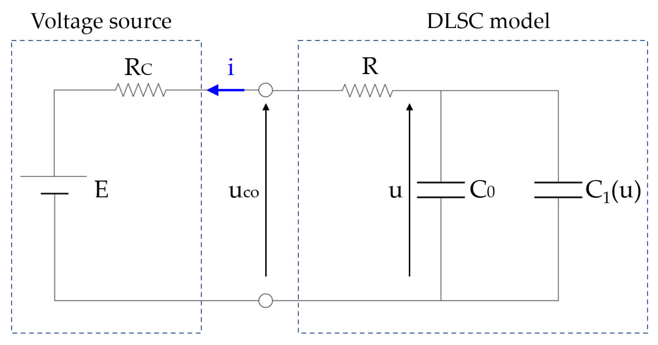
2.1. Electrical Analysis of a DLSC Charged or Discharged with a Voltage Source

This section will show how to express the different electrical variables of a DLSC when connected to a voltage source. The voltage source will be represented by a constant no load voltage, E, and a series connected resistor, R_C. As mentioned above, the supercapacitor model will be that of a capacitance linearly varying with its internal voltage. All the obtained functions will be valid for charging and discharging with a voltage source or discharging with a constant resistor. In the second case, it is sufficient to cancel the no-load voltage, E = 0 V, and the discharge resistance will be R_C. The internal resistance of the DLSC will be denoted as R and its capacitance will vary with the internal voltage called u. The external voltage of the DLSC is u_co and will obviously coincide with the terminal voltage of the voltage source (Figure 1).

The capacitance of the DLSC shall be modelled as the parallel association of two capacitances, one of constant value, C₀, called “Initial Capacitance”, which is the capacitance when the DLSC is fully discharged, and the other which is proportional to the internal voltage, C₁(u). The final capacitance of the cell, C(u), will be the parallel association of the two.

$$\mathrm{C}\left(\mathrm{u}\right)={\mathrm{C}}_0+{\mathrm{C}}_1\left(\mathrm{u}\right)={\mathrm{C}}_0+{\mathrm{k}}_{\mathrm{c}}·\mathrm{u}.$$

(1)

The values of C₀ and k_c are not specified in the datasheets of the cells provided by the manufacturers but can be expressed as a function of the rated capacitance, C_N, and the rated voltage, U_N. In this way, the capacitance can be expressed as a function of the internal voltage as follows:

$$\mathrm{C}\left(\mathrm{u}\right)={\mathrm{C}}_0+\frac{{\mathrm{C}}_{\mathrm{N}}}{{\mathrm{U}}_{\mathrm{N}}}·\left(1-\frac{{\mathrm{C}}_0}{{\mathrm{C}}_{\mathrm{N}}}\right)·\mathrm{u}={\mathrm{C}}_{\mathrm{N}}·{\mathrm{k}}_0+\frac{{\mathrm{C}}_{\mathrm{N}}}{{\mathrm{U}}_{\mathrm{N}}}·\left(1-{\mathrm{k}}_0\right)·\mathrm{u}.$$

(2)

The value of k₀ (dimensionless), which is the quotient of the initial capacitance and the nominal capacitance, is known as the “Normalized Initial Capacitance”. In a conventional capacitor, with constant capacitance, it is true that: k₀ = 1, k_c = 0 and C_N = C₀. The constant k₀ is also not usually specified in the datasheets, but in most families of SCs from different manufacturers, k₀ presents values between 0.7 and 0.8. Considering a discharge process, according to the definition of an electric current, this is equal to the time variation of charges experienced by the device, i.e.,

$$\mathrm{i}=-\frac{\mathrm{dq}}{\mathrm{dt}}=-\frac{\mathrm{dq}}{\mathrm{du}}·\frac{\mathrm{du}}{\mathrm{dt}}.$$

(3)

The negative sign indicates that the current represents a discharge. In both conventional SCs and DLSCs, the capacitance establishes the well-known relationship between electric charge and internal voltage:

$$\mathrm{q}=\mathrm{C}\left(\mathrm{u}\right)·\mathrm{u}.$$

(4)

Considering the capacitance value in (1), the stored charge can be expressed as a function of the internal voltage and the values of C₀ and k_c:

$$\mathrm{q}={\mathrm{C}}_0·\mathrm{u}+{\mathrm{k}}_{\mathrm{c}}·{\mathrm{u}}^2.$$

(5)

By deriving the charge q with respect to the internal voltage:

$$\frac{\mathrm{dq}}{\mathrm{du}}={\mathrm{C}}_0+2·{\mathrm{k}}_{\mathrm{c}}·\mathrm{u}.$$

(6)

If the value of the derivative calculated in (6) is substituted in the expression for the current, the relationship between the current and the internal voltage can be obtained:

$$\mathrm{i}=-\frac{\mathrm{dq}}{\mathrm{dt}}=-\underset{\mathrm{Virtual} \mathrm{Capacitance}}{\underbrace{\left({\mathrm{C}}_0+2·{\mathrm{k}}_{\mathrm{c}}·\mathrm{u}\right)}}·\frac{\mathrm{du}}{\mathrm{dt}}=-{ \mathrm{C}}_{\mathrm{v}}·\frac{\mathrm{du}}{\mathrm{dt}}.$$

(7)

The C_V value is called “Virtual Capacitance” or “Dynamic Capacitance”. When the DLSC is discharged through a voltage source, the following must also be fulfilled:

$${\mathrm{u}}_{\mathrm{co}}=\mathrm{E}+{\mathrm{R}}_{\mathrm{c}}·\mathrm{i}=\mathrm{u}-\mathrm{R}·\mathrm{i}.$$

(8)

Therefore, the value of the current will be the following:

$$\mathrm{i}=\frac{\mathrm{u}-\mathrm{E}}{{\mathrm{R}}_{\mathrm{c}}+\mathrm{R}}.$$

(9)

Substituting in (9) the value of the current obtained in (7) gives the following first-order differential equation of separate variables:

$$\frac{\mathrm{u}-\mathrm{E}}{{\mathrm{R}}_{\mathrm{c}}+\mathrm{R}}=-\left({\mathrm{C}}_0+2·{\mathrm{k}}_{\mathrm{c}}·\mathrm{u}\right)·\frac{\mathrm{du}}{\mathrm{dt}}.$$

(10)

Assuming that at t = 0, the DLSC starts from a known internal voltage of value u (t = 0) = U₀ (in the case of the discharge, it is satisfied that U₀ > E), and separating the two variables of (10), it is given that:

$${{\displaystyle \int }}_{{\mathrm{U}}_0}^{\mathrm{u}}\frac{{\mathrm{C}}_0+2·{\mathrm{k}}_{\mathrm{c}}·\mathrm{u}}{\mathrm{u}-\mathrm{E}}·\mathrm{du}={{\displaystyle \int }}_0^{\mathrm{t}}-\frac{\mathrm{dt}}{{\mathrm{R}}_{\mathrm{c}}+\mathrm{R}}.$$

(11)

By integrating (11), the following equality, where time is related to the value of internal voltage, is obtained:

$$\ln \left|\mathrm{u}-\mathrm{E}\right|+\frac{2·{\mathrm{k}}_{\mathrm{c}}·\mathrm{u}}{{\mathrm{C}}_0+2·{\mathrm{k}}_{\mathrm{c}}·\mathrm{E}}=\ln \left|{\mathrm{U}}_0-\mathrm{E}\right|+\frac{2·{\mathrm{k}}_{\mathrm{c}}·{\mathrm{U}}_0}{{\mathrm{C}}_0+2·{\mathrm{k}}_{\mathrm{c}}·\mathrm{E}}-\frac{\mathrm{t}}{\left({\mathrm{R}}_{\mathrm{c}}+\mathrm{R}\right)·\left({\mathrm{C}}_0+2·{\mathrm{k}}_{\mathrm{c}}·\mathrm{E}\right)}$$

(12)

During a charging process (E > U₀), it will also be true that E ≥ u, since the internal voltage can never exceed the value of the voltage source, and (12) would be equally valid. In order to simplify the mathematical development, two new constants, k₁ and k₂, will be defined:

$${\mathrm{k}}_1=\frac{2·{\mathrm{k}}_{\mathrm{c}}}{{\mathrm{C}}_0+2·{\mathrm{k}}_{\mathrm{c}}·\mathrm{E}},$$

(13)

$${\mathrm{k}}_2=\frac{1}{\left({\mathrm{R}}_{\mathrm{c}}+\mathrm{R}\right)·\left({\mathrm{C}}_0+2·{\mathrm{k}}_{\mathrm{c}}·\mathrm{E}\right)}.$$

(14)

k₁ is measured in V⁻¹ and k₂ in s⁻¹. Both constants shall be considered positive. The sign of the voltage source, E, cannot be negative since all SCs, such as electrolytic capacitors, only admit one polarity. If E were negative, the SC could reach an internal voltage of u < 0 which would irreversibly damage it.

By means of k₁ and k₂, (12) can be simplified as follows:

$$\ln \left|\mathrm{u}-\mathrm{E}\right|+{\mathrm{k}}_1·\mathrm{u}=\ln \left|{\mathrm{U}}_0-\mathrm{E}\right|+{\mathrm{k}}_1·{\mathrm{U}}_0-{\mathrm{k}}_2·\mathrm{t}.$$

(15)

The equality obtained in (15) shows the relationship between the internal voltage, u, and the time, t. From this equation, it is possible to obtain the internal voltage as a function of time, u(t):

$$\mathrm{u}\left(\mathrm{t}\right)=\mathrm{E}+\frac{1}{{\mathrm{k}}_1}·{\mathrm{W}}_0\left({\mathrm{k}}_1·\left({\mathrm{U}}_0-\mathrm{E}\right)·{\mathrm{e}}^{{\mathrm{k}}_1·\left({\mathrm{U}}_0-\mathrm{E}\right)-{\mathrm{k}}_2·\mathrm{t}}\right),$$

(16)

where W₀(x) represents the main or superior branch of the Lambert W function which will be used in both charging (E ≥ u) and discharging (E ≤ u), as will be latter explained. E, k₁ and U₀ make it possible to define a new constant, k₃:

$${\mathrm{k}}_3={\mathrm{k}}_1·\left({\mathrm{U}}_0-\mathrm{E}\right)·{\mathrm{e}}^{{\mathrm{k}}_1·\left({\mathrm{U}}_0-\mathrm{E}\right)}.$$

(17)

k₃ is dimensionless, positive at discharge (U₀ > E) and negative at charge (U₀ < E). The internal voltage, expressed as a function of this new constant, is as follows:

$$\mathrm{u}=\mathrm{E}+\frac{1}{{\mathrm{k}}_1}·{\mathrm{W}}_0\left({\mathrm{k}}_3·{\mathrm{e}}^{-{\mathrm{k}}_2·\mathrm{t}}\right).$$

(18)

In order to further simplify the rest of the mathematical analysis, a new function called g(t), measured in (V), will be defined with the following expression:

$$\mathrm{g}\left(\mathrm{t}\right)=\frac{1}{{\mathrm{k}}_1}·{\mathrm{W}}_0\left({\mathrm{k}}_3·{\mathrm{e}}^{-{\mathrm{k}}_2·\mathrm{t}}\right).$$

(19)

The internal voltage, u, expressed as a function of g, gives the following equation:

$$\mathrm{u}=\mathrm{E}+\mathrm{g}.$$

(20)

The expression of the variable g given in (19) is valid only for k_c > 0 (k₀ < 1). To model a conventional capacitor of constant capacity by using (20) and entering the value k₀ = 1 would lead to an indeterminacy. However, it can be shown that the same function would be obtained by using the classical formulas without more than taking into account that:

$$\underset{{\mathrm{k}}_0\to 1}{\lim }\mathrm{g}\left(\mathrm{t}\right)=\left({\mathrm{U}}_0-\mathrm{E}\right)·{\mathrm{e}}^{\frac{-\mathrm{t}}{\left({\mathrm{R}}_{\mathrm{c}}+\mathrm{R}\right)·{\mathrm{C}}_0}}$$

(21)

By means of (9) and (20), the discharge current as a function of g is also obtained:

$$\mathrm{i}=\frac{\mathrm{g}}{{\mathrm{R}}_{\mathrm{c}}+\mathrm{R}}$$

(22)

In the case of charging (E > u), it follows from (20) that the value of g will be negative, while during discharging, (u > E), g will always be positive. As in (22), the expression for the current supplied by the DLSC was presented, if E > u is satisfied, g will be negative, therefore the current will be absorbed by the DLSC.

As mentioned above, only the main branch of the Lambert W function, W₀(x), can be used. This restriction is caused by the fact that during a discharge, as time, t, increases, the argument x of the function W₀(x), presented in (19), is positive (k₃ > 0) and decreasing; for positive values of x, only the main branch of the function is defined (Figure 2). In this case, if time tends to infinity, the value of x will tend to zero; therefore, the value of g also tends to zero, so the internal voltage, u, will converge to the value of the voltage source E. During a charging process, since u < E, the argument of W₀(x) will be negative (k₃ < 0) and its absolute value will be decreasing. Consequently, as time increases, the absolute value |x| tends to zero, as do the functions W₀(–|x|) and g, and again, the internal voltage, u, will converge to the value of E, which is what must happen. If the secondary or lower branch of the Lambert W function, W_–1(–|x|), were taken as a solution, as |x| tends to zero, it would tend to –∞, as would the function g and hence the internal voltage of the DLSC, which would not make physical sense. Figure 2 shows the evolution of the variable g over time, both in the charging and discharging processes. In both cases, for very large values of time, t, the variable g will tend to zero, which will be its limiting value.

On the other hand, from Equations (8) and (22), it is easy to deduce the value of the external voltage as a function of the variable g:

$${\mathrm{u}}_{\mathrm{co}}=\mathrm{E}+\left(\frac{{\mathrm{R}}_{\mathrm{c}}}{{\mathrm{R}}_{\mathrm{c}}+\mathrm{R}}\right)·\mathrm{g}.$$

(23)

The power dissipated as heat in the internal resistance R of the DLSC, p_d, can also be expressed as a function of the variable g in the following way:

$${\mathrm{p}}_{\mathrm{d}}=\mathrm{R}·{\mathrm{i}}^2=\frac{\mathrm{R}}{{\left({\mathrm{R}}_{\mathrm{c}}+\mathrm{R}\right)}^2}·{\mathrm{g}}^2.$$

(24)

Similarly, the power dissipated in the internal resistance of the voltage source, R_c, presents the same function as p_d, changing R to R_c; that is:

$${\mathrm{p}}_{\mathrm{dRc}}=\frac{{\mathrm{R}}_{\mathrm{c}}}{{\left({\mathrm{R}}_{\mathrm{c}}+\mathrm{R}\right)}^2}·{\mathrm{g}}^2.$$

(25)

The power absorbed by the voltage source, E, representing the no-load voltage of the voltage source is:

$${\mathrm{p}}_{\mathrm{E}}=\mathrm{E}·\mathrm{i}=\left(\frac{\mathrm{E}}{{\mathrm{R}}_{\mathrm{c}}+\mathrm{R}}\right)·\mathrm{g}.$$

(26)

The output power of the DLSC, i.e., the power consumed by the voltage source, p_out, is obtained by simply multiplying the external voltage by the current; therefore:

$${\mathrm{p}}_{\mathrm{out}}={\mathrm{u}}_{\mathrm{co}}·\mathrm{i}=\left(\frac{\mathrm{E}}{{\mathrm{R}}_{\mathrm{c}}+\mathrm{R}}\right)·\mathrm{g}+\frac{{\mathrm{R}}_{\mathrm{c}}}{{\left({\mathrm{R}}_{\mathrm{c}}+\mathrm{R}\right)}^2}·{\mathrm{g}}^2.$$

(27)

The energy dissipated in the internal resistance, R, of the DLSC, e_d, is obtained by integrating the power loss, p_d, obtained in (24). In doing so, it is considered that:

$${\mathrm{p}}_{\mathrm{d}}=\frac{{\mathrm{de}}_{\mathrm{d}}}{\mathrm{dt}}=\frac{{\mathrm{de}}_{\mathrm{d}}}{\mathrm{dg}}·\frac{\mathrm{dg}}{\mathrm{dt}}.$$

(28)

Deriving g(t) as a function of time, as presented in (19), after some simplifications, it is obtained that:

$$\mathrm{g} \prime =\frac{\mathrm{dg}}{\mathrm{dt}}=\frac{-\mathrm{g}}{\left({\mathrm{R}}_{\mathrm{c}}+\mathrm{R}\right)·\left({\mathrm{C}}_0+2·{\mathrm{k}}_{\mathrm{c}}·\mathrm{E}+2·{\mathrm{k}}_{\mathrm{c}}·\mathrm{g}\right)}.$$

(29)

The expression for g’ in (29) is valid for both charging and discharging, without the need to change the sign. If the value g’ obtained in (29) and the value of p_d calculated in (24) are substituted into (28), integrating both members of the obtained equation, the result is the value of the energy dissipated in the resistance R, e_d, depending on the variable g:

$${\mathrm{e}}_{\mathrm{d}}=\frac{\mathrm{R}·\left({\mathrm{C}}_0+2·{\mathrm{k}}_{\mathrm{c}}·\mathrm{E}\right)}{2·\left({\mathrm{R}}_{\mathrm{c}}+\mathrm{R}\right)}·\left({{\mathrm{g}}_0}^2-{\mathrm{g}}^2\right)+\frac{2·{\mathrm{k}}_{\mathrm{c}}·\mathrm{R}}{3·\left({\mathrm{R}}_{\mathrm{c}}+\mathrm{R}\right)}·\left({{\mathrm{g}}_0}^3-{\mathrm{g}}^3\right).$$

(30)

In the expression given in (30), g₀ is the value of $\mathrm{g}$ evaluated in t = 0 that, according to (20), results in g₀ = U₀ − E. The energy dissipated in ${\mathrm{R}}_{\mathrm{c}}$, e_dRc, follows the same evolution as e_d, by only changing the value of R that appears in the numerators by R_c, i.e.,

$${\mathrm{e}}_{\mathrm{dRc}}=\frac{{\mathrm{R}}_{\mathrm{c}}·\left({\mathrm{C}}_0+2·{\mathrm{k}}_{\mathrm{c}}·\mathrm{E}\right)}{2·\left({\mathrm{R}}_{\mathrm{c}}+\mathrm{R}\right)}·\left({{\mathrm{g}}_0}^2-{\mathrm{g}}^2\right)+\frac{2·{\mathrm{k}}_{\mathrm{c}}·{\mathrm{R}}_{\mathrm{c}}}{3·\left({\mathrm{R}}_{\mathrm{c}}+\mathrm{R}\right)}·\left({{\mathrm{g}}_0}^3-{\mathrm{g}}^3\right).$$

(31)

Another variable that is important to consider is the instantaneous energy stored in the DLSC. This energy depends on the constants ${\mathrm{C}}_0$, ${\mathrm{k}}_{\mathrm{c}}$ and the internal voltage, u, according to the following equation:

$${\mathrm{e}}_{\mathrm{stored}}=\frac{1}{2}·\left({\mathrm{C}}_0+\frac{4}{3}·{\mathrm{k}}_{\mathrm{c}}·\mathrm{u}\right)·{\mathrm{u}}^2=\frac{1}{2}·{\mathrm{C}}_{\mathrm{E}}·{\mathrm{u}}^2.$$

(32)

The C_E value is called “Energetic Capacitance”, as it is used to obtain the energy stored in a variable capacitance DLSC, with an equation similar to that used in a conventional capacitor. This, as with the dynamic capacitance, also depends on the internal voltage. By substituting the former (20) in (32), the instantaneous stored energy as a function of g is finally obtained:

$${\mathrm{e}}_{\mathrm{stored}}=\frac{1}{2}·{\mathrm{C}}_0·{\left(\mathrm{E}+\mathrm{g}\right)}^2+\frac{2}{3}·{\mathrm{k}}_{\mathrm{c}}·{\left(\mathrm{E}+\mathrm{g}\right)}^3.$$

(33)

If the DLSC starts from an initial internal voltage, U₀, and after a time, t, reaches an internal voltage, u, the discharged energy, e_dch, will be:

$${\mathrm{e}}_{\mathrm{dch}}=\frac{1}{2}·{\mathrm{C}}_0·\left({\mathrm{U}}_0^2-{\left(\mathrm{E}+\mathrm{g}\right)}^2\right)+\frac{2}{3}·{\mathrm{k}}_{\mathrm{c}}·\left({\mathrm{U}}_0^3-{\left(\mathrm{E}+\mathrm{g}\right)}^3\right).$$

(34)

On the other hand, the energy consumed by the voltage source, E, e_E, can be also obtained by integration, bearing in mind that:

$${\mathrm{p}}_{\mathrm{E}}=\frac{{\mathrm{de}}_{\mathrm{E}}}{\mathrm{dt}}=\frac{{\mathrm{de}}_{\mathrm{E}}}{\mathrm{dg}}·\frac{\mathrm{dg}}{\mathrm{dt}}.$$

(35)

Replacing in (35) the value of p_E as a function of g, obtained in (26), and the value of the derivative of g(t) with respect to time, calculated in (29), and integrating the energy consumed or generated, depending on whether it is a charge or discharge of the DLSC can be obtained:

$${\mathrm{e}}_{\mathrm{E}}=\mathrm{E}·\left({\mathrm{C}}_0+2·{\mathrm{k}}_{\mathrm{c}}·\mathrm{E}\right)·\left({\mathrm{g}}_0-\mathrm{g}\right)+{\mathrm{k}}_{\mathrm{c}}·\mathrm{E}·\left({{\mathrm{g}}_0}^2-{\mathrm{g}}^2\right).$$

(36)

Finally, it is necessary to develop an equation that expresses time as a function of g. The variable g as a function of time was calculated earlier in (19). From the definition of the Lambert W function itself, it must be satisfied that:

$${\mathrm{k}}_1·\mathrm{g}·{\mathrm{e}}^{{\mathrm{k}}_1·\mathrm{g}}={\mathrm{k}}_3·{\mathrm{e}}^{-{\mathrm{k}}_2·\mathrm{t}}.$$

(37)

Taking neperian logarithms on both sides of (37), the function t(g) is obtained:

$$\mathrm{t}=\frac{1}{{\mathrm{k}}_2}·\ln \left(\frac{{\mathrm{k}}_3}{{\mathrm{k}}_1·\mathrm{g}}\right)-\frac{{\mathrm{k}}_1}{{\mathrm{k}}_2}·\mathrm{g}.$$

(38)

By replacing k₁, k₂ and k₃, previously and respectively calculated in (13), (14) and (17) in (38), the time, t, can be expressed as a function of g and other known variables:

$$\mathrm{t}=2·{\mathrm{k}}_{\mathrm{c}}·\left({\mathrm{R}}_{\mathrm{c}}+\mathrm{R}\right)·\left[\left(\frac{{\mathrm{C}}_0}{2·{\mathrm{k}}_{\mathrm{c}}}+\mathrm{E}\right)·\ln \left(\frac{{\mathrm{U}}_0-\mathrm{E}}{\mathrm{g}}\right)+{\mathrm{U}}_0-\mathrm{E}-\mathrm{g}\right].$$

(39)

As can be deduced from (39), for g to reach a zero value, the time, t, should tend to infinity. As in first-order circuits with conventional capacitors that are charged or discharged through a voltage source, the time constant, τ, can be defined as the elapsed time for the following equality to be satisfied, valid for both charging and discharging (e being the Euler’s number):

$$\mathrm{u}-\mathrm{E}=\left({\mathrm{U}}_0-\mathrm{E}\right)·{\mathrm{e}}^{-1}.$$

(40)

Considering the value of t obtained in (39) and the relationship between g, u and E from (20), the “time constant” of the circuit, τ, can be determined by the following equation:

$$\mathsf{\tau }=\left({\mathrm{R}}_{\mathrm{c}}+\mathrm{R}\right)·\left({\mathrm{C}}_0+2·{\mathrm{k}}_{\mathrm{c}}·\left({\mathrm{U}}_0+\frac{\mathrm{E}-{\mathrm{U}}_0}{\mathrm{e}}\right)\right).$$

(41)

In contrast to conventional capacitors, the time constant is not only dependent on the passive elements but is also a function of the initial voltage of the DLSC, U₀ and the no-load voltage, E, of the source. This result is congruent, since for this model, the capacitance of the DLSC is a function with linear dependence on its internal voltage, whereas in a conventional capacitor, the capacitance remains invariant.

2.2. Mathematical Expresión of g as a Function of the Electrical Variables

Once a set of equations has been obtained with the main electrical variables and time as a function of the variable g, the complementary equations of g, as a function of the current, voltage, power and so on, will be calculated. In this way, the development of analytical equations will be completed, obtaining a set of functions where any variable can be expressed as a function of the others. The variable g as a function of time has already been found in Equation (19). The calculation of g as a function of internal voltage is immediate if (20) is used:

$$\mathrm{g}=\mathrm{u}-\mathrm{E} .$$

(42)

The calculation of g as a function of the current is straightforward from (22):

$$\mathrm{g}=\mathrm{i}·\left({\mathrm{R}}_{\mathrm{c}}+\mathrm{R}\right).$$

(43)

Similarly, g can also be obtained as a function of the external voltage by simply using (23):

$$\mathrm{g}=\left(1+\frac{\mathrm{R}}{{\mathrm{R}}_{\mathrm{c}}}\right)·\left({\mathrm{u}}_{\mathrm{co}}-\mathrm{E}\right).$$

(44)

By means of (24), g can be expressed as a function of the power dissipated in the internal resistance of the DLSC, p_d.

$$\mathrm{g}=\left({\mathrm{R}}_{\mathrm{c}}+\mathrm{R}\right)·\sqrt{\frac{{\mathrm{p}}_{\mathrm{d}}}{\mathrm{R}}}.$$

(45)

As in (45), the value of g as a function of the power dissipated in the resistance of the voltage source R_c, p_dRc, has the same form but replaces the value of R by R_c; thus:

$$\mathrm{g}=\left({\mathrm{R}}_{\mathrm{c}}+\mathrm{R}\right)·\sqrt{\frac{{\mathrm{p}}_{\mathrm{dRc}}}{{\mathrm{R}}_{\mathrm{c}}}}.$$

(46)

The expression for g as a function of the power consumed by E, p_E, is also directly obtained from (26):

$$\mathrm{g}=\left({\mathrm{R}}_{\mathrm{c}}+\mathrm{R}\right)·\left(\frac{{\mathrm{p}}_{\mathrm{E}}}{\mathrm{E}}\right).$$

(47)

To express g as a function of the DLSC output power, p_out, it is necessary to solve the second-degree equation shown in (27). Of the two possible solutions, the positive one must be chosen both in the charging and discharging cases:

$$\mathrm{g}=\frac{\mathrm{E}}{2}·\left(1+\frac{\mathrm{R}}{{\mathrm{R}}_{\mathrm{c}}}\right)·\left(-1+\sqrt{1+\frac{4·{\mathrm{R}}_{\mathrm{c}}·{\mathrm{p}}_{\mathrm{out}}}{{\mathrm{E}}^2}}\right).$$

(48)

The equation of g as a function of the energy dissipated by the source, E, e_E, is obtained in almost the same way, by solving the second-degree equation obtained in (36) and also choosing the positive solution:

$$\mathrm{g}=-\mathrm{E}-\frac{{\mathrm{C}}_0}{2·{\mathrm{k}}_{\mathrm{c}}}+\frac{1}{2}·\sqrt{{\left(\frac{{\mathrm{C}}_0}{{\mathrm{k}}_{\mathrm{c}}}+2·\left(\mathrm{E}+{\mathrm{g}}_0\right)\right)}^2-\frac{4·{\mathrm{e}}_{\mathrm{E}}}{\mathrm{E}·{\mathrm{k}}_{\mathrm{c}}}}.$$

(49)

Obtaining expressions of g as a function of e_dch, e_stored, e_d and e_dRc is more complex, since all four are cubic functions of g. They have therefore been omitted from this study, since, in addition, the set of analytical expressions already shown and their combinations allow practically all possible alternatives to be covered. For example, if the value of the internal voltage of the DLSC, u, as a function of the power consumed by the voltage source E, p_E, is to be calculated, it would be sufficient to combine (20), where u(g) is defined, with (47), which presents the equation of $\mathrm{g}\left({\mathrm{p}}_{\mathrm{E}}\right)$. The equation of $\mathrm{u}\left({\mathrm{p}}_{\mathrm{E}}\right)$, would be directly obtained:

$$\mathrm{u}=\mathrm{E}+\left({\mathrm{R}}_{\mathrm{c}}+\mathrm{R}\right)·\left(\frac{{\mathrm{p}}_{\mathrm{E}}}{\mathrm{E}}\right).$$

(50)

If the objective was to calculate the time it would take for the external voltage, u_co, to reach a certain value, i.e., to obtain the function t(u_co), the combination of (39), which defines t(g), and (44) which shows g(u_co), would directly yield t(u_co):

$$\mathrm{t}=2·{\mathrm{k}}_{\mathrm{c}}·\left({\mathrm{R}}_{\mathrm{c}}+\mathrm{R}\right)·\left[\left(\frac{{\mathrm{C}}_0}{2·{\mathrm{k}}_{\mathrm{c}}}+\mathrm{E}\right)·\ln \left(\frac{{\mathrm{R}}_{\mathrm{c}}}{{\mathrm{R}}_{\mathrm{c}}+\mathrm{R}}·\frac{{\mathrm{U}}_0-\mathrm{E}}{{\mathrm{u}}_{\mathrm{co}}-\mathrm{E}}\right)+{\mathrm{U}}_0-{\mathrm{u}}_{\mathrm{co}}+\frac{\mathrm{R}}{{\mathrm{R}}_{\mathrm{c}}}·\left(\mathrm{E}-{\mathrm{u}}_{\mathrm{co}}\right)\right]$$

(51)

As in the previous two examples, the process can be repeated with any two electrical variables (it is possible to include time, t) and to obtain an analytical expression of the associated function.

3. Results and Discussion

This section will show a case study in which a DLSC, modelled as a capacitance linearly varying with the internal voltage, will be charged through a voltage source. The evolution of the electrical variables will be studied using the set of analytical expressions of Section 2, and simulations will be carried out to analyze their variation with different values of the constant k₀. Subsequently, the results obtained will be compared with the same DLSC, considering it as a constant capacitance with its equivalent series resistance.

Table 1. Rated values of the selected DLSC.

E (V)	UN (V)	U0 (V)	R (mΩ)	CN (F)
2.7	2.7	0	25	25

shows its rated data together with the no-load voltage of the voltage source, E.

The wiring diagram of the case study is presented in Figure 3.

To study the time evolution of the different variables, three values will be considered for the variable k₀ = [0.65, 0.85, 1] and four different values will be chosen for the internal resistance of the voltage source, R_c (Ω) = [0.5, 1, 3, 5]. From the obtained results, the constants C₀, k_c, k₁, k₂ and k₃ as defined in Equations (2), (13), (14) and (17) will be, respectively, calculated together with the value of the time constant, τ, according to (41), which, in this study, is the time taken for the internal voltage to reach 1.7067 V. All the above values are shown in

Table 2. Constants C₀, k_c, k₁, k₂, k₃ and τ for different values of k₀ and R_c.

Case	k0	C0 (F)	kc (F·V−1)	Rc (Ω)	k1 (V−1)	k2 (s−1)	k3	τ (s)
1	0.65	16.25	3.2407	0.5	0.1920	0.0564	–0.3087	11.911
4				1		0.0289		23.255
7				3		0.0098		68.631
10				5		0.0059		114.07
2	0.85	21.25	1.3889	0.5	0.0966	0.0663	–0.2010	12.605
5				1		0.0339		24.609
8				3		0.0115		72.627
11				5		0.0069		120.64
3	1	25	0	0.5	0	0.0762	0	13.125
6				1		0.0390		25.625
9				3		0.0132		75.625
12				5		0.0080		125.62

.

Figure 4 shows the evolution of the DLSC internal voltage, u(t), for different values of the constant k₀ and various values of the internal resistance of the voltage source, R_c. As can be appreciated from it, for the three models of different k₀, there is a coincidence in three values of the internal voltage, u(t). Two of them are obvious, since they are the initial value (they all start from the same U₀) and the final value, which converge to the no-load voltage of the voltage source E = U_N = 2.7 V. The third one corresponds to a specific value of the g variable. This value, which will be denoted as g_s, ensures that whatever the value of k₀ and the resistance, R_c, it will be the same in all models. The value of g_s can be calculated as follows:

$${\mathrm{g}}_{\mathrm{s}}=\left(\mathrm{E}-\frac{{\mathrm{U}}_{\mathrm{N}}}{2}\right)·{\mathrm{W}}_0\left(\frac{{\mathrm{U}}_0-\mathrm{E}}{\mathrm{E}-\frac{{\mathrm{U}}_{\mathrm{N}}}{2}}·\exp \left(\frac{{\mathrm{U}}_0-\mathrm{E}}{\mathrm{E}-\frac{{\mathrm{U}}_{\mathrm{N}}}{2}}\right)\right).$$

(52)

As shown in (52), g_s only depends on E, the rated voltage of the cell, U_N and its initial voltage, U₀, but is independent of all other variables, including R_c. In the case study presented, g_s = −0.5486 V. If this value of g_s is replaced in (20), where u(g) was calculated, the internal voltage at which all the models coincide is 2.1514 V, as can be appreciated from Figure 4. Below this voltage, the variable capacitance model (k₀ < 1) produces higher internal voltages than the conventional model, while beyond this point, the trend is reversed. By substituting this value of g_s in (39), the result is the time instant at which, for any value of k₀, all the internal voltages cross at a common point. This instant does depend on the value of R_c.

Table 3. Time instants at which the internal voltage u = 2.1514 V is the same for different values of k₀ and R_c, and current values, i(t) (A), at those instants.

	Rc (Ω)
	0.5	1	3	5
t (s)	20.92	40.84	120.52	200.2
i (A)	–1.0449	–0.5352	–0.1814	–0.1092

shows the times at which, with all the models, the same internal voltage is reached as a function of the values of R_c. The value of the current at those instants is also displayed.

Figure 5 shows the difference between the calculation of the internal voltage with variable capacitance, k₀ = [0.65, 0.85], and the conventional model with constant capacitance, k₀ = 1, for different values of R_c. As can be seen, the maximum difference is independent of the value taken by R_c, which only affects the instant at which it appears. In this example, the maximum discrepancy between the conventional DLSC model and the one with k₀ = 0.65 is 0.1738 V.

Figure 6 shows the evolution of the instantaneous current of the circuit, i(t), calculated with the three values of the constant k₀ and for different values of R_c. In the same instants in which the internal voltage, u, coincides, the current also coincides, whatever the value of k₀, although in this case, the values of the current are different for each Rc value, since i(t) depends on this resistance, as was earlier indicated by means of expression (9). It can be observed how, in the calculation of the current, the difference between modelling the DLSC with variable capacitance and with constant capacitance is minimal. It can therefore be concluded that the usual RC series model is perfectly valid for i(t) calculation.

Figure 7 shows the difference between the current obtained with variable capacitance, k₀ = [0.65, 0.85], and the conventional model with constant capacitance, k₀ = 1, for different values of R_c. As can be appreciated, the higher the value of R_c, the less difference there is between considering the model with variable capacitance and the RC series model with constant capacitance.

Figure 8 shows the time evolution of the energy dissipated in the internal resistance of the DLSC, e_d(t), presented in (30) and calculated with the three values of the constant k₀ and different values of R_c. The higher the value of the constant k₀, at any instant of time, the higher the energy dissipated. Furthermore, the larger the value of R_c the smaller the difference between models with different k₀ values. Finally, Figure 9 shows the difference in the energy dissipated in the DLSC, e_d(t), displayed in absolute value, between the model with variable capacitance, k₀ = [0.65, 0.85], and conventional capacitor, k₀ = 1, considering different values of R_c.

4. Conclusions

The main electrical variables of a DLSC, modelled as a capacitance linearly varying with the internal voltage, when charged or discharged through a voltage source, have been obtained. The set of analytical expressions presented is equally useful for the case in which the DLSC is discharged through a constant resistance, as occurs in industrial applications such as instantaneous heaters, or if it is desired to analyze the self-discharge process. Furthermore, from the new set of equations, the time constant of the DLSC has been defined by resemblance to conventional, constant capacitance capacitors. Unlike other more sophisticated models, which are valuable and very accurate, even in the representation of the physical structure of the DLSC, the set of analytical equations presented here is not restricted to the use of numerical calculation tools. It also allows analytical solutions to be easily obtained without the complexity involved in the models mentioned, where complex tools, from distributed parameter circuits to artificial neural networks, are used.

It is often claimed that the series RC model does not accurately model the behavior of a DLSC. Therefore, in this paper, a comparative study between the model with variable capacitance (k₀ < 1) and the conventional model with constant capacitance (k₀ = 1) has been carried out and several conclusions have been drawn. It can be finally concluded that when a DLSC is connected to a voltage source, the differences between the models with k₀ < 1 and with k₀ = 1 are not too relevant, and the traditional RC series model, which is simpler and more widely used, provides, in most cases, sufficiently good values so that it is not necessary to treat it as a variable capacitance SC. In the case of needing to improve accuracy and/or perform direct analytical calculations, the new set of analytical equations developed here can be applied in a straightforward and very simple way.

References

1. Zhang, L.; Hu, X.; Wang, Z.; Sun, F.; Dorrell, D.G. A review of supercapacitor modeling, estimation, and applications: A control/management perspective. Renew. Sustain. Energy Rev. 2018, 81, 1868–1878. [Google Scholar]
2. Thounthong, P.; Raël, S.; Davat, B. Analysis of supercapacitor as second source based on fuel cell power generation. IEEE Trans. Energy Convers. 2009, 24, 247–255. [Google Scholar] [CrossRef]
3. Gyawali, N.; Ohsawa, Y. Integrating fuel/electrolyzer/ultracapacitor system into a stand-alone microhydro plant. IEEE Trans. Energy Convers. 2010, 25, 1092–1101. [Google Scholar]
4. Mellincovsky, M.; Kuperman, A.; Lerman, C.; Gadelovits, S.; Aharon, I.; Reichbach, N.; Geula, G.; Nakash, R. Performance and limitations of a constant power-fed supercapacitor. IEEE Trans. Energy Convers. 2014, 29, 445–452. [Google Scholar]
5. Zhang, L.; Hu, X.; Wang, Z.; Sun, F.; Deng, J.; Dorrell, D.G. Multiobjective optimal sizing of hybrid energy storage system for electric vehicles. IEEE Trans. Veh. Technol. 2018, 67, 1027–1035. [Google Scholar]
6. Zhao, C.; Yin, H.; Yang, Z.; Ma, C. Equivalent series resistance–based energy loss analysis of a battery semiactive hybrid energy storage system. IEEE Trans. Energy Convers. 2015, 30, 1081–1091. [Google Scholar]
7. Pedrayes, J.F.; Melero, M.G.; Cano, J.M.; Norniella, J.G.; Duque, S.B.; Rojas, C.H.; Orcajo, G.A. Lambert W function based closed–form expressions of supercapacitor electrical variables in constant power applications. Energy J. 2021, 218, 119364. [Google Scholar] [CrossRef]
8. Pedrayes, J.F.; Melero, M.G.; Norniella, J.G.; Cano, J.M.; Cabanas, M.F.; Orcajo, G.A.; Rojas, C.H. A novel analytical solution for the calculation of temperature in supercapacitors operating at constant power. Energy J. 2019, 188, 116047. [Google Scholar]
9. Pedrayes, J.F.; Melero, M.G.; Norniella, J.G.; Cabanas, M.F.; Orcajo, G.A.; González, A.S. Supercapacitors in Constant-Power Applications: Mathematical Analysis for the Calculation of Temperature. Appl. Sci. 2021, 11, 10153. [Google Scholar] [CrossRef]
10. Pedrayes, J.F.; Melero, M.G.; Cano, J.M.; Norniella, J.G.; Orcajo, G.A.; Cabanas, M.F.; Rojas, C.H. Optimization of supercapacitor sizing for high-fluctuating power applications by means of an internal-voltage-based method. Energy J. 2019, 183, 504–513. [Google Scholar]
11. Pedrayes, J.F.; Melero, M.G.; Cabanas, M.F.; Quintana, M.F.; Orcajo, G.A.; González, A.S. Sizing Methodology of a Fast Charger for Public Service Electric Vehicles Based on Supercapacitors. Appl. Sci. 2023, 13, 5398. [Google Scholar] [CrossRef]
12. Musolino, V.; Piegari, L.; Tironi, E. New full-frequency-range supercapacitor model with easy identification procedure. IEEE Trans. Ind. Electron. 2013, 60, 112–120. [Google Scholar] [CrossRef]
13. Shi, L.; Crow, M.L. Comparison of ultracapacitor electric circuit models. In Proceedings of the IEEE Power and Energy Society General Meeting—Conversion and Delivery of Electrical Energy in the 21st Century, Pittsburgh, PA, USA, 20–24 July 2008; pp. 1–6. [Google Scholar]
14. Pean, C.; Rotenberg, B.; Simon, P.; Salanne, M. Multi-scale modelling of supercapacitors: From molecular simulations to a transmission line model. J. Power Sources 2016, 326, 680–685. [Google Scholar] [CrossRef]
15. Zubieta, L.; Bonert, R. Characterization of double-layer capacitors for power electronics applications. IEEE Trans. Ind. Appl. 2000, 36, 199–205. [Google Scholar] [CrossRef]
16. Devillers, N.; Jemei, S.; Péra, C.; Bienaimé, D.; Gustin, F. Review of characterization methods for supercapacitor modelling. J. Power Sources 2014, 246, 596–608. [Google Scholar] [CrossRef]
17. Yang, H.; Zhang, Y. Self-discharge analysis and characterization of supercapacitors for environmentally powered wireless sensor network applications. J. Power Sources 2011, 196, 8866–8873. [Google Scholar] [CrossRef]
18. Marín-Coca, S.; Ostadrahimi, A.; Bifaretti, S.; Roibás, E.; Pindado, S. New Parameter Identification Method for Supercapacitor Model. IEEE Access 2023, 11, 21771–21782. [Google Scholar] [CrossRef]
19. Rufer, A.; Barrade, P. A supercapacitor-based energy-storage system for elevators with soft commutated interface. IEEE Trans. Ind. Appl. 2002, 38, 1151–1159. [Google Scholar] [CrossRef]
20. Reema, N.; Jagadan, G.; Sasidharan, N.; Shreelakshmi, M.P. Comparative Analysis of CC–CV/CC Charging and Charge Redistribution in Supercapacitors. In Proceedings of the 31st Australasian Universities Power Engineering Conference (AUPEC), Perth, Australia, 26–30 September 2021; pp. 1–5. [Google Scholar]
21. Li, H.; Zhang, X.; Peng, J.; He, J.; Huang, Z.; Wang, J. Cooperative CC–CV Charging of Supercapacitors Using Multicharger Systems. IEEE Trans. Ind. Electron. 2020, 67, 10497–10508. [Google Scholar] [CrossRef]
22. Zhang, X.; Liao, Y.; Li, H.; Liu, Y.; Zhang, R.; Meng, Z.; Peng, J.; Huang, Z. Consensus Control for CC–CV Charging of Supercapacitors. In Proceedings of the IEEE Energy Conversion Congress and Exposition (ECCE), Baltimore, MD, USA, 29 September–3 October 2019; pp. 2015–2020. [Google Scholar]
23. Ibrahim, T.; Stroe, D.; Kerekes, T.; Sera, D.; Spataru, S. An overview of supercapacitors for integrated PV—Energy storage panels. In Proceedings of the IEEE 19th International Power Electronics and Motion Control Conference (PEMC), Gliwice, Poland, 25–29 April 2021; pp. 828–835. [Google Scholar]
24. Dong, P.; Rodrigues, M.T.F.; Zhang, J.; Borges, R.S.; Kalaga, K.; Reddy, A.L.M.; Silva, G.G.; Ajayan, P.M.; Lou, J. A flexible solar cell/supercapacitor integrated energy device. Nano Energy 2017, 42, 181–186. [Google Scholar] [CrossRef]
25. Milan, S.; Vračar, J.; Vračar, L. Different Ways to Charging Supercapacitor in WSN Using Solar Cells. In Proceedings of the 7th International Conference on Electrical, Electronic and Computing Engineering, IcETRAN, Palembang, Indonesia, 6–9 June 2022; pp. 28–29. [Google Scholar]
26. Liu, J.; Zhang, W.; Rizzoni, G. Robust Stability Analysis of DC Microgrids with Constant Power Loads. IEEE Trans. Power Syst. 2018, 33, 851–860. [Google Scholar] [CrossRef]
27. Herrera, L.; Zhang, W.; Wang, J. Stability Analysis and Controller Design of DC Microgrids With Constant Power Loads. IEEE Trans. Smart Grid 2017, 8, 881–888. [Google Scholar]
28. Hassan, M.A.; Li, E.-P.; Li, X.; Li, T.; Duan, C.; Chi, S. Adaptive Passivity-Based Control of dc–dc Buck Power Converter with Constant Power Load in DC Microgrid Systems. IEEE J. Emerg. Sel. Top. Power Electron. 2019, 7, 2029–2040. [Google Scholar] [CrossRef]
29. Kularatna, N.; Gattuso, A.; Gurusinghe, N.; Jayasuriya, T.; Toit, J.D. Pre-stored supercapacitor energy as a solution for burst energy requirements in domestic in-line fast water heating systems. In Proceedings of the IECON 2014—40th Annual Conference of the IEEE Industrial Electronics Society, Dallas, TX, USA, 29 October–1 November 2014; pp. 3163–3167. [Google Scholar]
30. Kindracki, J.; Paszkiewicz, P.; Mężyk, Ł. Resistojet thruster with supercapacitor power source-design and experimental research. Aerosp. Sci. Technol. 2019, 92, 847–857. [Google Scholar] [CrossRef]
31. Fouda, M.E.; Allagui, A.; Elwakil, A.S.; Eltawil, A.; Kurdahi, F. Supercapacitor discharge under constant resistance, constant current and constant power loads. J. Power Sources 2019, 435, 226829. [Google Scholar] [CrossRef]
32. Xu, D.; Zhang, L.; Wang, B.; Ma, G. Modeling of Supercapacitor Behavior with an Improved Two-Branch Equivalent Circuit. IEEE Access 2019, 7, 26379–26390. [Google Scholar] [CrossRef]
33. Gould, J.E.; Chang, H. Estimations of compatibility of supercapacitors for use as power sources for resistance welding guns. Weld World 2013, 57, 887–894. [Google Scholar] [CrossRef]
34. Pentegov, I.; Sydorets, V.; Bondarenko, I.; Bondarenko, O.; Safronov, P. Estimation of supercapacitor efficiency in use for resistance welding. In Proceedings of the 2015 16th International Conference on Computational Problems of Electrical Engineering (CPEE), Lviv, Ukraine, 2–5 September 2015; pp. 142–145. [Google Scholar]
35. Fernando, J.; Kularatna, N.; Silva, S.; Thotabaddadurage, S.S. Supercapacitor assisted surge absorber technique: High performance transient surge protectors for consumer electronics. IEEE Power Electron. Mag. 2022, 9, 48–60. [Google Scholar] [CrossRef]
36. Kularatna, N.; Subasinghage, K.; Gunawardane, K.; Jayananda, D.; Ariyarathna, T. Supercapacitor-Assisted Techniques and Supercapacitor-Assisted Loss Management Concept: New Design Approaches to Change the Roadmap of Power Conversion Systems. Electronics 2021, 10, 1697. [Google Scholar] [CrossRef]
37. Kularatna, N.; Fernando, J.; Pandey, A. Surge endurance capability testing of supercapacitor families. In Proceedings of the IECON 2010—36th Annual Conference on IEEE Industrial Electronics Society, Glendale, AZ, USA, 7–10 November 2010; pp. 1858–1863. [Google Scholar]
38. Thotabaddadurage, S.U.S.; Kularatna, N.; Steyn, D.A. Permeance Based Design and Analysis of Supercapacitor Assisted Surge Absorber for Magnetic Component Selection. IEEE Trans. Ind. Electron. 2023, 70, 3593–3603. [Google Scholar] [CrossRef]
Figure 1. Discharge of the DLSC through a voltage source.
Applsci 13 06714 g001
Figure 2. Evolution of the variable g over time, during charging and discharging processes.
Applsci 13 06714 g002
Figure 3. Wiring diagram of the case study.
Applsci 13 06714 g003
Figure 4. Evolution of the internal voltage of the DLSC, u(t), for different values of k0 and Rc. The points marked with a rhombus indicate the value of the internal voltage that is equal for all values of k0 and Rc.
Applsci 13 06714 g004
Figure 5. Differences of the internal voltage, u(t), displayed in absolute value, between the model with variable capacitance, k0 = [0.65, 0.85], and the conventional capacitor with constant capacitance, k0 = 1, and considering different values of Rc.
Applsci 13 06714 g005
Figure 6. Instantaneous current, i(t) (A), for different values of k0 and Rc.
Applsci 13 06714 g006
Figure 7. Differences of the current, i(t), displayed in absolute value, between the model with variable capacitance, k0 = [0.65, 0.85], and the conventional capacitor with constant capacitance, k0 = 1, and considering different values of Rc.
Applsci 13 06714 g007
Figure 8. Evolution of the energy dissipated in the DLSC, ed(t) (J), for different values of k0 and Rc.
Applsci 13 06714 g008
Figure 9. Differences in the energy dissipated in the DLSC, ed(t), displayed in absolute value, between the model with variable capacitance, k0 = [0.65, 0.85], and the conventional capacitor, k0 = 1, considering different values of Rc.
Applsci 13 06714 g009