An Advanced Crow Search Algorithm for Solving Global Optimization Problem

Abstract

The conventional crow search (CS) algorithm is a swarm-based metaheuristic algorithm that has fewer parameters, is easy to apply to problems, and is utilized in various fields. However, it has a disadvantage, as it is easy for it to fall into local minima by relying mainly on exploitation to find approximations. Therefore, in this paper, we propose the advanced crow search (ACS) algorithm, which improves the conventional CS algorithm and solves the global optimization problem. The ACS algorithm has three differences from the conventional CS algorithm. First, we propose using dynamic $AP$ (awareness probability) to perform exploration of the global region for the selection of the initial population. Second, we improved the exploitation performance by introducing a formula that probabilistically selects the best crows instead of randomly selecting them. Third, we improved the exploration phase by adding an equation for local search. The ACS algorithm proposed in this paper has improved exploitation and exploration performance over other metaheuristic algorithms in both unimodal and multimodal benchmark functions, and it found the most optimal solutions in five engineering problems.

1. Introduction

The optimization of engineering problems is of great interest to many researchers, and various strategies for incorporating optimization into the engineering field are being studied [1]. As an example, metaheuristic algorithms that are easy to apply to engineering problems are being developed for optimization. These algorithms are applied to various fields in order to optimize engineering problems by minimizing costs, shortening paths, and maximizing performance.

Metaheuristic algorithms originated in 1965 with the development of the evolution strategy (ES) algorithm [2], and algorithms using various natural phenomena have been proposed. Figure 1 classifies the metaheuristic algorithms based on the natural phenomena that they emulate. Metaheuristic algorithms can be classified into four main categories: evolutionary, swarm, physic, and human behavior [3,4,5,6,7]. Evolution-based algorithms are based on the genetic characteristics and evolutionary methods of nature, and representative algorithms include ES, evolutionary programming (EP), genetic algorithm (GA), genetic programming (GP), and differential evolution (DE). Swarm-based algorithms are based on the behavior of organisms such as birds or ants in clusters, and representative algorithms include ant colony optimization (ACO), particle swarm optimization (PSO), artificial bee colony (ABC), cuckoo search, and crow search (CS). Physical-based algorithms are based on physical phenomena, and representative algorithms include simulated annealing (SA), harmony search (HS), gravitational search (GS), black hole (BH), and sine cosine (SC). Finally, the human behavior-based algorithms are based on human intelligent behavior, and representative algorithms include human-inspired (HI), social emotional optimization (SEO), brain storm optimization (BSO), teaching learning-based optimization (TLBO), and social-based (SB) [8]. All metaheuristic algorithms perform optimization using exploitation and exploration. If the metaheuristic algorithm mainly uses exploration, then it can easily find the global minima but has a difficult time finding the exact solution. Conversely, metaheuristic algorithms which mainly use exploitation can find accurate solutions but are prone to falling into local minima [9,10,11]. Therefore, the convergence performance of the algorithm varies greatly depending on the method of using exploitation and exploration, and exploitation and exploration should be used in harmony [12].

Swarm-based algorithms are efficient in searching for global optima and are easy to apply to a variety of optimization problems. They also lend themselves well to parallelization, making them a popular choice for many researchers [13]. With these advantages, swarm-based algorithms are applied to various engineering fields, and many researchers are working to improve the convergence performance of algorithms. The conventional CS algorithm, originally proposed by Askarzadeh in 2016 and ranked among the swarm-based algorithms, performs optimization by mimicking the high intelligence of crows [14]. Crow brains are intelligent enough to recognize food or humans because they are large compared to their body size. As crows are intelligent, they can remember the location of food hidden by other birds and steal this hidden food when the other birds are not around. The conventional CS algorithm proposes to perform optimization using these characteristics of crows and has the following four principles:

• Crows live in groups.
• Crows remember the location of their hidden prey.
• Crows steal food from other birds.
• Crows are protected by probability.

The conventional CS algorithm utilizes a small number of parameters and demonstrates excellent convergence performance. Due to its easy application in problems and excellent performance, it is widely applied in civil and architectural engineering, electrical engineering, mechanical engineering, and image processing [15]. The conventional CS algorithm is more likely to fall into local minima because it mainly performs optimization using exploitation rather than exploration. However, given that real optimization problems are often characterized by multimodal functions, optimization algorithms should mainly use exploration rather than exploitation to find accurate solutions [16]. In order to address this issue, Mohammadi et al. proposed a modified crow search (MCS) algorithm in 2018 that performs optimization through the adoption of a new method for selecting a target crow as well as variation of $fl$ (flight length) based on distance depending on the distance of the crow [17]. In the same year, Díaz et al. proposed the improved crow search (ICS) algorithm, which is improved by random adoption methods using $AP$ (awareness probability) and Lévy flight varying by fitness in the t generation [18]. $AP$ is one of the important parameters used in the conventional CS algorithms, and depending on the size of the $AP$, the conventional CS algorithms perform exploitation or exploration. In 2019, Zamani et al. proposed the conscious neighborhood-based crow search (CCS) algorithm, which utilizes three strategies: neighborhood-based local search (NLS), non-neighborhood-based global search (NGS), and wandering around-based search (WAS) [19]. In the same year, Javidi et al. proposed the enhanced crow search (ECS) algorithm [20], which used three additional mechanisms. In addition, the convergence performance of the ECS algorithm was evaluated compared to the conventional CS algorithm to which three mechanisms were applied. In 2020, Wu et al. proposed the Lévy flight crow search (LFCS) algorithm combining Lévy flight and the conventional CS algorithm [21]. Recently, in 2022, Necira et al. proposed the dynamic crow search (DCS) algorithm, and it utilizes $AP$, which linearly decreases with the number of generations, and $fl$, which is randomly selected by the parity probability density function [22].

In this paper, the advanced crow search (ACS) algorithm was proposed as a means to solve the global optimization problem. The ACS algorithm uses $dynamicAP$—which varies nonlinearly with changes in the number of generations—and suggests that we follow the best results of previous generations with a probability-based approach, rather than randomly chasing the prey selected by crows. In addition, instead of randomly selecting from the entire problem range, the algorithm proposes reducing the randomly selected space as the number of generations increases. Section 2 briefly reviews conventional CS algorithms and papers that improve on these conventional CS algorithms, and Section 3 compares the explanation of the ACS algorithm with the convergence performance according to parameter changes. In Section 4, we solve the numerical optimization problem and compare the results with those of other algorithms. Section 5 presents the conclusions drawn from this study.

2. Related Work

In this section, we explain the process of optimizing the conventional CS algorithm and briefly outline research projects that have improved upon the conventional CS algorithm.

2.1. Conventional CS Algorithm

The conventional CS algorithm proposed by Askarzadeh describes the intelligent behavior of crows and performs optimization by repeating the following five steps [14]:

Step 1. Define the problem and set the parameters

The problem undergoing optimization is defined, and the initial value of the parameters used in the conventional CS algorithm are set. The parameters used in the conventional CS algorithms are $AP$ (awareness probability), $fl$ (flight length), N (flock size), $pd$ (dimension of problem), and $t_{max}$ (maximum number of generations).

Step 2. Initialize the memory of crows and evaluate

The size of the crow group, determined by $pd$ and the size of N, is expressed as Equation (1), and the initial position of each crow is randomly assigned within the range between $lb$ (lower boundary) and $ub$ (upper boundary). In this context, i is $1,2,\dots ,N$, t are $1,2,\dots ,t_{max}$, and d is $pd$. The initial position of the randomly placed crow is remembered as Equation (2), and the initial position of the crow is evaluated by object function.

$$\begin{array}{c}\hfill Crow{s}_{i,t}=\left[\begin{array}{ccc}{x}_i^1& \cdots & x_i^d\\ ⋮& ⋮& ⋮\\ x_N^1& \cdots & x_N^d\end{array}\right]\end{array}$$

(1)

$$\begin{array}{c}\hfill CrowsMemor{y}_{i,t}=\left[\begin{array}{ccc}{m}_i^1& \cdots & m_i^d\\ ⋮& ⋮& ⋮\\ m_N^1& \cdots & m_N^d\end{array}\right]\end{array}$$

(2)

Step 3. Generate and evaluate the new positions for crows

Step 3 is the most important step that the conventional CS algorithm uses to perform optimization. Crow i ($x_{i,t}$) follows crow j ($m_{j,t}$), and two cases are proposed depending on whether crow j is aware of crow i’s following. The first case is that crow j ($m_{j,t}$) does not recognize crow i ($x_{i,t}$)’s following. The position of crow i ($x_{i,t}$) is adjusted by Equation (3), where $r_i$ is a random number between 0 and 1. In addition, a local ($fl$ < 1) or global ($fl$ > 1) area search is performed depending on the size of $fl$, and it is known to have the best convergence performance when using $fl$ = 2.0. Figure 2 is a diagram that expresses this characteristic.

$$\begin{array}{c}\hfill x_{i,t+1}=x_{i,t}+r_i\times fl\times (m_{j,t}-x_{i,t})\end{array}$$

(3)

$$\begin{array}{c}\hfill x_{i,t+1}=arandomposition\end{array}$$

(4)

The second case is that crow j ($m_{j,t}$) recognizes crow i ($x_{i,t}$)’s following. In this instance, the position of crow i is adjusted by Equation (4), moving to a random position in the range between $lb$ and $ub$. Two cases are selected from each generation by the $AP$, and the $AP$ mainly uses 0.1. Relative to the size of $AP$, the conventional CS algorithms perform exploitation and exploration in order to find the optimal solutions. The positions of the newly moved crows are again evaluated by the objective function.

Step 4. Update the memory

The results are compared by evaluating the crow position change using Equations (3) and (4) with the evaluation of crows stored in memory. Comparing the evaluation results, the better crow position is updated in the crow’s memory.

Step 5. Termination of repetition

The process of Steps 2–4 is repeated continuously, and when t reaches $t_{max}$, the performance of the conventional CS algorithm is terminated in order to derive optimization results. The pseudo code of the above-mentioned process is provided in Algorithm 1.

Algorithm 1 Pseudo code of the conventional CS algorithm

Initialize the parameters($AP$, $fl$, N, $pd$, $t_{max}$) Initialize the position of crows in the search space and memorize Evaluate the position of crows while $t<t_{max}$do     Randomly choose the position of crows     for $i=1:N$ do         if $r_i\ge AP$ then            $x_{i,t+1}=x_{i,t}+r_i\times fl\times (m_{j,t}-x_{i,t})$         else            $x_{i,t+1}=arandomposition$         end if     end for     Evaluate the new position of crows     Update the memory of crows end while Show the results

2.2. Modified CS Algorithm

The modified CS (MCS) algorithm was proposed by Mohammadi et al. in 2018 [17]. The MCS algorithm has a similar structure compared to the conventional CS algorithm, but two new equations have been proposed.

First, MCS algorithm uses K parameters, which use random variables between ‘0’ and ‘1’ to select the target crow (Crow j), unlike the conventional CS algorithm. K is defined as Equation (5) and consists of $K_{max}$ and $K_{min}$. K has values that decrease with the number of generations by $K_{max}$ and $K_{min}$.

$$\begin{array}{c}\hfill K_t=round\left(K_{max}-\frac{K_{max}-K_{min}}{t_{max}}\times t\right)\end{array}$$

(5)

If K has a large value, then the probability that a crow in a bad position will be selected increases; if K has a small value, then the probability that the crow in the best position will be selected increases. Therefore, exploration is primarily performed in the initial generations, and exploitation is primarily performed in the latter generations.

Second, the MCS algorithm uses a value of $fl$ differently depending on the distance between crow i and crow j, where $fl$ is defined as Equation (6). Here, $f{l}_{thr}$ and $D_{thr}$ are initially set parameters, and $D_{i,j}$ is the distance vector of crow i and crow j.

$$\begin{array}{c}\hfill f{l}_{i,t}=\left\{\begin{array}{ccc}2& if& D_{i,j}>D_{thr}\\ f{l}_{thr}& if& D_{i,j}\le D_{thr}\end{array}\right.\end{array}$$

(6)

Askarzadeh noted that when $fl$ = 2, the conventional CS algorithm has the best convergence performance [14]. However, the MCS algorithm uses $f{l}_{i,t}$ with a value greater than 2 when the crow’s distance ($D_{i,j}$) is closer than $D_{thr}$.

2.3. Dynamic CS Algorithm

The dynamic CS (DCS) algorithm was proposed by Necira et al. in 2022 [22], and it proposed dynamic $AP$ and $fl$ that change with the number of generations.

First, dynamic $AP$, which varies dynamically with the number of generations, is defined as Equation (7). dynamic $AP$ decreases linearly within the range of $A{P}_{max}$ and $A{P}_{min}$ as the number of generations increases. This change causes the initial number of generations to perform the exploration in the global search space.

$$\begin{array}{c}\hfill AP=A{P}_{max}+\frac{A{P}_{max}-A{P}_{min}}{t_{max}}\times t\end{array}$$

(7)

Second, $f{l}_c$ was used instead of $fl$ used by the conventional CS algorithm, which is defined as Equation (8). The conventional CS algorithm initially determines $fl$ and performs a local search or global search based on the determined value. However, DCS algorithm mainly performs a global search when it is less than a certain number of generations, and a local search when it exceeds a certain number of generations. These changes are determined by $\tau$ and are mainly used at 0.9.

$$\begin{array}{c}\hfill f{l}_c=\left\{\begin{array}{cccc}& fl\times \left[F\left(\frac{y_{max}}{10}\right)-F\left(y_{min}\right)\times r\right]& if& t\le \tau \times t_{max}\\ & fl\times \left[F\left(y_{max}\right)-F\left(y_{max}\right)-F\left(0.6\times y_{max}\right)\right]& else\end{array}\right.\end{array}$$

(8)

3. Proposed Method

3.1. Advanced CS Algorithm

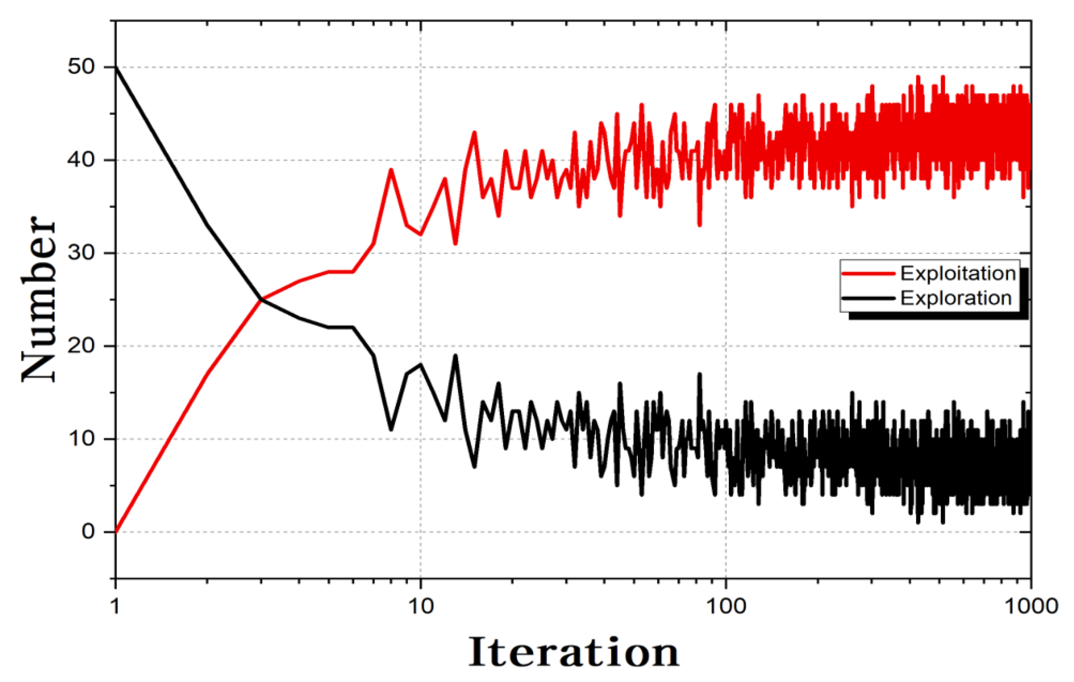
The conventional CS algorithm, which repeats the above process to perform optimization, performs exploration and exploitation according to the size of $AP$, mainly using 0.1 for $AP$. That is, the conventional CS algorithm mainly performs the exploitation rather than the exploration. Figure 3 is a diagram showing the exploitation and exploration that occurs in the process of optimizing the Sphere function for 1000 generations of the conventional CS algorithms with a N of 50. It can be seen that exploitation mainly occurs in all generations. Optimization algorithms that mainly use excitation in optimization performance are likely to fall into local minima [10], and the performance of the conventional CS algorithms is largely dependent on the initial population. In this paper, to address this problem, we improve the performance of the initial population using dynamic $AP$ that varies dynamically with the number of generations, and  the performance of exploitation and exploration using two proposed equations.

Similar to the conventional CS algorithm, the ACS algorithm consists of a total of five steps.

Step 1. Define the problem and set the parameters

Like the conventional CS algorithm, the problem for performing optimization is defined in Step 1, and the parameters used in the ACS algorithm are set. The parameters added in the ACS algorithm are $A{P}_{max}$, $A{P}_{min}$, and $FAR$ (Flight Awareness Ratio). Here, $A{P}_{max}$ and $A{P}_{min}$ are used for dynamic $AP$.

Step 2. Initialize the memory of crows and evaluate

The size of the crew group used in the ACS algorithm is expressed as Equation (1) as in the conventional CS algorithm, and the initial position is remembered as Equation (2). The initial position of the remembered crow is evaluated by the objective function.

Step 3. Generate and evaluate the new positions for crows

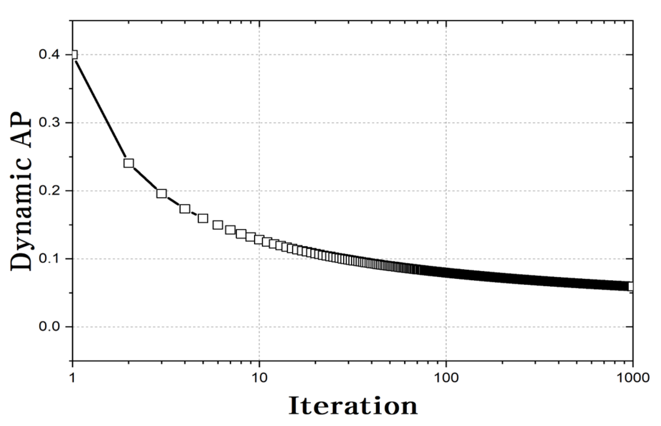
The ACS algorithm displays the biggest difference from the conventional CS algorithm in Step 3. First, The ACS algorithm uses dynamic $AP$, which changes dynamically with the number of generations. dynamic $AP$ uses Equation (9) for dynamic changes, and $A{P}_{max}$ and $A{P}_{min}$ have a value between 0 and 1. Figure 4 shows an $AP$ that changes dynamically according to the number of generations when $t_{max}$ is 2000. Using dynamic $AP$, as shown in Figure 5, increases the probability of exploration at the beginning of the generation, which can increase the performance of the initial population. Compared to Figure 3, the number of explorations increases at lower numbers of generations. Thus, the larger the AP, the higher the probability of the initial population performing exploration, and the smaller the AP, the higher the probability of performing exploitation. In addition, a dynamic $AP$ of an appropriate size is required for harmony between exploitation and exploration.

$$\begin{array}{c}\hfill A{P}_t=A{P}_{min}+\frac{A{P}_{max}-A{P}_{min}}{ln\left(t\right)+1}\end{array}$$

(9)

Second, unlike the conventional Equation (3) in which crow i follows randomly selected crow j ($m_{j,t}$), in the ACS algorithm, it follows the best crow j ($g{b}_{j,t}$) by $FAR$. This can be expressed as Equation (10). Here, $r_{i,t}^2$, $r_{i,t}^3$ is a random number between 0 and 1, and $FAR$ is an initial set value between 0 and 1. The change in this equation improves the exploitation performance compared to the conventional CS algorithm. If $FAR$ approaches 0, it follows the best solution stored in the crow’s memory. Conversely, when $FAR$ approaches 1, it follows a randomly selected crow, just like the conventional CS algorithm. Therefore, using the appropriate $FAR$, it is possible to improve the convergence performance of the optimization algorithm by harmonizing the exploitation and exploration.

$$\begin{array}{c}\hfill x_{i,t+1}=\left\{\begin{array}{ccc}{x}_{i,t}+r_{i,t}^2\times fl\times (m_{j,t}-x_{j,t})& & r_{i,t}^3\le FAR\\ x_{i,t}+r_{i,t}^2\times fl\times (g{b}_{j,t}-x_{j,t})& & else\end{array}\right.\end{array}$$

(10)

Third, using this algorithm, the exploration phase of the conventional CS algorithm was improved. The conventional CS algorithms are randomly adopted in the $lb$ and $ub$ ranges if the random number is less than the $AP$. That is, global search is mainly performed. The global search can contribute to the convergence performance of the algorithm because it searches a large area at the beginning of the generation. However, it does not contribute significantly to the convergence performance of the algorithm as the generation progresses. Therefore, the process of reducing the range that can be selected toward the end of the generation was added as Equation (11), which allows the ACS algorithm to perform a local search. Here, $r_{i,t}^4$ and $r_{i,t}^5$ are random numbers between 0 and 1. Figure 6 illustrates this method.

$$\begin{array}{c}\hfill x_{i,t+1}=\left\{\begin{array}{ccc}2x_{i,t}+(lb+r_{i,t}^5\times (lb-ub))/t& & r_{i,t}^4<0.5\\ arandomposition& & else\end{array}\right.\end{array}$$

(11)

Step 4. Update the memory

The results are compared through evaluation of the crow position change by Equation (3), Equation (4) with the evaluation of crows stored in memory. Comparing the evaluation results, the better crow position is updated in the crow’s memory.

Step 5. Termination of repetition

The ACS algorithm performs optimization by repeating the process of Steps 2–4. When the current number of generations (t) reaches the maximum number of generations ($t_{max}$), the execution of the ACS algorithm ends, and the optimization result of the problem is derived. Pseudo code of the above-mentioned process is provided in Algorithm 2.

Algorithm 2 Pseudo code of the ACS algorithm

Initialize the parameters($A{P}_{max}$, $A{P}_{min}$, $FAR$, $fl$, N, $pd$, $t_{max}$) Initialize the position of crows in the search space and memorize Evaluate the position of crows while $t<t_{max}$do     Randomly choose the position of crows     for $i=1:N$ do         if $r_{i,t}^1\ge A{P}_t$ then            if $r_{i,t}^3\le FAR$ then                $x_{i,t+1}=x_{i,t}+r_{i,t}^2\times fl\times (m_{j,t}-x_{i,t})$            else                $x_{i,t+1}=x_{i,t}+r_{i,t}^2\times fl\times (g{b}_{j,t}-x_{i,t})$            end if         else            if $r_{i,t}^4\le 0.5$ then                $x_{i,t+1}=2x_{i,t}+(lb+r_{i,t}^5\times (lb-ub))/t$            else                $x_{i,t+1}=arandomposition$            end if         end if     end for     Evaluate the new position of crows     Update the memory of crows end while Show the results

3.2. Characteristic of the ACS Algorithm

Unlike the conventional CS algorithm, the ACS algorithm adds the parameters of $dynamic$ $AP$ and $FAR$. Therefore, this section compares the convergence performance according to the change in the newly added parameters and seeks the value with the best convergence performance. The benchmark function was used to compare convergence performance, and it was summarized in

Table 1. Benchmark function for comparison.

Fun	Equation	B	Min
f1	$f\left(x\right)={\sum }_{i=1}^n{x}_i^2$	[−100 100] ${}^d$	0
f2	$f\left(x\right)={\sum }_{i=1}^n\left|x_i\right|+{\prod }_{i=1}^n\left|x_i\right|$	[−10 10] ${}^d$	0
f3	$f\left(x\right)={\sum }_{i=1}^n{\left({\sum }_{j-1}^i{x}_j\right)}^2$	[−100 100] ${}^d$	0
f4	$f\left(x\right)=max\left\{\left|x_i\right|,1\le i\le n\right\}$	[−100 100] ${}^d$	0
f5	$f\left(x\right)={\sum }_{i=1}^{n-1}\left[100{\left(x_{i=1}-x_i^2\right)}^2+{\left(x_i-1\right)}^2\right]$	[−30 30] ${}^d$	0
f6	$f\left(x\right)={\sum }_{i=1}^n{\left(\left[x_i+0.5\right]\right)}^2$	[−100 100] ${}^d$	0
f7	$f\left(x\right)={\sum }_{i=1}^{n}i{x}_i^4+rand\left(0,1\right)$	[−1.28 1.28] ${}^d$	0
f8	$f\left(x\right)={\sum }_{i=1}^n-xsin\sqrt{\left|x_i\right|}$	[−500 500] ${}^d$	$-418.9829\times d$
f9	$f\left(x\right)={\sum }_{i=1}^n\left[x_i^2-10cos\left(2\pi x_i\right)\right]+10$	[−5.12 5.12] ${}^d$	0
f10	$f\left(x\right)=-20exp\left(-0.2\sqrt{\frac{1}{n}{\sum }_{i=1}^n{x}_i^2}\right)-exp\left(\frac{1}{n}{\sum }_{i=1}^{n}cos\left(2\pi x_i\right)\right)+20+e$	[−32 32] ${}^d$	0
f11	$f\left(x\right)=\frac{1}{4000}{\sum }_{i=1}^n{x}_i^2-{\prod }_{i=1}^{n}cos\left(\frac{x_i}{\sqrt{i}}\right)$	[−600 600] ${}^d$	0
f12	$f\left(x\right)=\frac{\pi }{n}\left\{10{sin}^2\left(\pi y_1\right)+{\sum }_{i=1}^{n-1}{(y_i-1)}^2\left[1+10{sin}^2\left(\pi y_{i+1}\right)\right]+{(y_n-1)}^2\right\}+{\sum }_{i=1}^{n}u(x_i,a,k,m)$	[−50 50] ${}^d$	0
f13	$f\left(x\right)=0.1\left\{{sin}^2\left(3\pi x_1\right)+{\sum }_{i=1}^{n-1}{(x_i-1)}^2\left[1+{sin}^2\left(3\pi x_{i+1}\right)\right]+{(x_n-1)}^2\left[1+{sin}^2\left(2\pi x_n\right)\right]\right\}+{\sum }_{i=1}^{n}u(x_i,a,k,m)$	[−50 50] ${}^d$	0

. Here, d was set to 10 in order to identify the characteristics of the ACS algorithm.

A total of 13 functions were used to compare the convergence performance according to the value of the added parameter. In Table 1, f1–f7 is a unimodal benchmark function that can test the exploitation performance of each algorithm. Additionally, f8–f13 is a multimodal benchmark function that can test the exploration performance of each algorithm. The multimodal benchmark function has many local minima, making it difficult to find an exact solution.

3.2.1. $DynamicAP$

The ACS algorithm uses $dynamicAP$, which varies with the number of generations, to increase the performance of the exploration initially. $dynamicAP$ is calculated by Equation (9) and has a different value depending on the size of the $A{P}_{max}$. Figure 7 is a graph that changes according to the size of the $A{P}_{max}$. The larger the $A{P}_{max}$, the higher the probability of randomly selecting the entire boundary initially and the better the initial population selection. Therefore, this section compares results that change according to the value of the $A{P}_{max}$.

When $AP$ becomes 0, only exploitation occurs in all generations. Therefore, the $A{P}_{min}$ was set to a minimum value of (=0.01). $A{P}_{max}$ was changed to 0.01, 0.1, 0.2, 0.4, 0.6, 0.8, and 1.0, and N, $fl$, and $FAR$ were set to 20, 2.0, and 1.0. $t_{max}$ was set to 2000, and each analysis was repeated a total of 50 times.

Table 2. Benchmark function results according to $A{P}_{max}$.

Fun	Index	${\mathit{AP}}_{\mathit{max}}$
		0.01	0.1	0.2	0.4	0.6	0.8	1.0
f1	BF	1.539 $\times {10}^{-16}$	2.262 $\times {10}^{-25}$	2.565 $\times {10}^{-26}$	2.593 $\times {10}^{-24}$	1.061 $\times {10}^{-21}$	1.529 $\times {10}^{-18}$	2.833 $\times {10}^{-17}$
	MF	1.210 $\times {10}^{-11}$	3.174 $\times {10}^{-20}$	4.473 $\times {10}^{-22}$	2.924 $\times {10}^{-21}$	1.009 $\times {10}^{-18}$	2.040 $\times {10}^{-16}$	1.780 $\times {10}^{-14}$
	Std	3.856 $\times {10}^{-11}$	1.148 $\times {10}^{-19}$	2.366 $\times {10}^{-21}$	6.870 $\times {10}^{-21}$	2.496 $\times {10}^{-18}$	3.732 $\times {10}^{-16}$	3.336 $\times {10}^{-14}$
f2	BF	9.000 $\times {10}^{-4}$	2.982 $\times {10}^{-7}$	3.825 $\times {10}^{-9}$	1.453 $\times {10}^{-9}$	2.523 $\times {10}^{-8}$	5.769 $\times {10}^{-8}$	4.234 $\times {10}^{-7}$
	MF	4.804 $\times {10}^{-1}$	3.235 $\times {10}^{-1}$	5.726 $\times {10}^{-2}$	5.967 $\times {10}^{-3}$	3.480 $\times {10}^{-3}$	1.651 $\times {10}^{-3}$	1.669 $\times {10}^{-2}$
	Std	8.730 $\times {10}^{-1}$	6.932 $\times {10}^{-1}$	1.713 $\times {10}^{-1}$	2.146 $\times {10}^{-2}$	1.474 $\times {10}^{-2}$	6.987 $\times {10}^{-3}$	5.230 $\times {10}^{-2}$
f3	BF	8.264 $\times {10}^{-7}$	3.387 $\times {10}^{-12}$	3.318 $\times {10}^{-15}$	1.478 $\times {10}^{-15}$	6.072 $\times {10}^{-14}$	3.762 $\times {10}^{-13}$	9.214 $\times {10}^{-11}$
	MF	7.755 $\times {10}^{-4}$	3.325 $\times {10}^{-8}$	2.260 $\times {10}^{-10}$	2.695 $\times {10}^{-12}$	1.810 $\times {10}^{-11}$	1.778 $\times {10}^{-10}$	2.906 $\times {10}^{-9}$
	Std	1.426 $\times {10}^{-3}$	8.402 $\times {10}^{-8}$	1.294 $\times {10}^{-9}$	4.797 $\times {10}^{-12}$	3.574 $\times {10}^{-11}$	3.233 $\times {10}^{-10}$	7.114 $\times {10}^{-9}$
f4	BF	6.825 $\times {10}^{-4}$	1.288 $\times {10}^{-6}$	7.312 $\times {10}^{-8}$	5.775 $\times {10}^{-8}$	3.196 $\times {10}^{-8}$	4.060 $\times {10}^{-7}$	1.179 $\times {10}^{-6}$
	MF	2.281 $\times {10}^{-1}$	1.375 $\times {10}^{-3}$	4.209 $\times {10}^{-5}$	3.244 $\times {10}^{-6}$	3.038 $\times {10}^{-6}$	1.968 $\times {10}^{-5}$	3.329 $\times {10}^{-5}$
	Std	5.381 $\times {10}^{-1}$	5.247 $\times {10}^{-3}$	1.190 $\times {10}^{-4}$	9.829 $\times {10}^{-6}$	4.470 $\times {10}^{-6}$	5.200 $\times {10}^{-5}$	5.856 $\times {10}^{-5}$
f5	BF	1.713 $\times {10}^0$	4.013 $\times {10}^{-1}$	5.917 $\times {10}^{-1}$	3.408 $\times {10}^{-1}$	8.382 $\times {10}^{-2}$	1.636 $\times {10}^{-1}$	2.719 $\times {10}^{-1}$
	MF	4.907 $\times {10}^1$	3.163 $\times {10}^1$	1.235 $\times {10}^1$	5.890 $\times {10}^0$	1.942 $\times {10}^1$	4.255 $\times {10}^0$	6.337 $\times {10}^0$
	Std	1.146 $\times {10}^2$	7.602 $\times {10}^1$	3.155 $\times {10}^1$	1.722 $\times {10}^1$	6.666 $\times {10}^1$	1.329 $\times {10}^1$	1.842 $\times {10}^1$
f6	BF	1.153 $\times {10}^{-15}$	4.338 $\times {10}^{-25}$	1.302 $\times {10}^{-26}$	8.952 $\times {10}^{-24}$	1.329 $\times {10}^{-21}$	3.406 $\times {10}^{-18}$	4.081 $\times {10}^{-16}$
	MF	1.516 $\times {10}^{-11}$	1.065 $\times {10}^{-20}$	5.884 $\times {10}^{-23}$	3.664 $\times {10}^{-21}$	5.147 $\times {10}^{-19}$	1.780 $\times {10}^{-16}$	2.082 $\times {10}^{-14}$
	Std	8.877 $\times {10}^{-11}$	3.800 $\times {10}^{-20}$	1.452 $\times {10}^{-22}$	1.099 $\times {10}^{-20}$	6.811 $\times {10}^{-19}$	3.103 $\times {10}^{-16}$	2.444 $\times {10}^{-14}$
f7	BF	3.638 $\times {10}^{-3}$	1.402 $\times {10}^{-3}$	2.790 $\times {10}^{-4}$	2.662 $\times {10}^{-4}$	4.150 $\times {10}^{-4}$	5.504 $\times {10}^{-4}$	5.838 $\times {10}^{-4}$
	MF	1.861 $\times {10}^{-2}$	7.457 $\times {10}^{-3}$	5.353 $\times {10}^{-3}$	3.847 $\times {10}^{-3}$	3.338 $\times {10}^{-3}$	3.086 $\times {10}^{-3}$	3.419 $\times {10}^{-3}$
	Std	1.243 $\times {10}^{-2}$	4.381 $\times {10}^{-3}$	3.128 $\times {10}^{-3}$	2.699 $\times {10}^{-3}$	2.168 $\times {10}^{-3}$	1.838 $\times {10}^{-3}$	2.241 $\times {10}^{-3}$
f8	BF	−3.475 $\times {10}^3$	−3.517 $\times {10}^3$	−3.616 $\times {10}^3$	−3.835 $\times {10}^3$	−3.736 $\times {10}^3$	−3.617 $\times {10}^3$	−3.476 $\times {10}^3$
	MF	−2.618 $\times {10}^3$	−2.790 $\times {10}^3$	−2.784 $\times {10}^3$	−2.797 $\times {10}^3$	−2.799 $\times {10}^3$	−2.911 $\times {10}^3$	−2.816 $\times {10}^3$
	Std	4.082 $\times {10}^2$	3.450 $\times {10}^2$	3.783 $\times {10}^2$	3.988 $\times {10}^2$	3.896 $\times {10}^2$	3.289 $\times {10}^2$	3.013 $\times {10}^2$
f9	BF	5.970 $\times {10}^0$	4.975 $\times {10}^0$	5.970 $\times {10}^0$	4.975 $\times {10}^0$	3.980 $\times {10}^0$	5.970 $\times {10}^0$	5.970 $\times {10}^0$
	MF	2.507 $\times {10}^1$	2.454 $\times {10}^1$	2.366 $\times {10}^1$	2.306 $\times {10}^1$	2.255 $\times {10}^1$	2.312 $\times {10}^1$	1.988 $\times {10}^1$
	Std	1.058 $\times {10}^1$	1.282 $\times {10}^1$	1.374 $\times {10}^1$	1.166 $\times {10}^1$	1.164 $\times {10}^1$	1.061 $\times {10}^1$	1.095 $\times {10}^1$
f10	BF	2.013 $\times {10}^0$	1.150 $\times {10}^{-5}$	1.131 $\times {10}^{-12}$	2.077 $\times {10}^{-11}$	1.267 $\times {10}^{-10}$	2.340 $\times {10}^{-9}$	1.762 $\times {10}^{-8}$
	MF	3.965 $\times {10}^0$	2.984 $\times {10}^0$	2.625 $\times {10}^0$	2.436 $\times {10}^0$	2.361 $\times {10}^0$	2.100 $\times {10}^0$	2.096 $\times {10}^0$
	Std	1.073 $\times {10}^0$	1.097 $\times {10}^0$	8.876 $\times {10}^{-1}$	9.702 $\times {10}^{-1}$	8.554 $\times {10}^{-1}$	9.932 $\times {10}^{-1}$	1.000 $\times {10}^0$
f11	BF	7.874 $\times {10}^{-2}$	7.378 $\times {10}^{-2}$	5.899 $\times {10}^{-2}$	6.637 $\times {10}^{-2}$	9.106 $\times {10}^{-2}$	8.115 $\times {10}^{-2}$	7.132 $\times {10}^{-2}$
	MF	7.107 $\times {10}^{-1}$	7.328 $\times {10}^{-1}$	5.611 $\times {10}^{-1}$	3.788 $\times {10}^{-1}$	4.330 $\times {10}^{-1}$	3.077 $\times {10}^{-1}$	2.621 $\times {10}^{-1}$
	Std	4.147 $\times {10}^{-1}$	3.670 $\times {10}^{-1}$	3.402 $\times {10}^{-1}$	2.323 $\times {10}^{-1}$	2.936 $\times {10}^{-1}$	1.644 $\times {10}^{-1}$	1.784 $\times {10}^{-1}$
f12	BF	2.089 $\times {10}^{-3}$	1.272 $\times {10}^{-5}$	2.475 $\times {10}^{-15}$	1.017 $\times {10}^{-16}$	2.176 $\times {10}^{-15}$	3.198 $\times {10}^{-14}$	2.542 $\times {10}^{-12}$
	MF	1.001 $\times {10}^1$	6.269 $\times {10}^0$	6.160 $\times {10}^0$	2.527 $\times {10}^0$	1.988 $\times {10}^0$	1.685 $\times {10}^0$	2.078 $\times {10}^0$
	Std	7.024 $\times {10}^0$	5.187 $\times {10}^0$	6.034 $\times {10}^0$	3.390 $\times {10}^0$	3.928 $\times {10}^0$	3.189 $\times {10}^0$	3.076 $\times {10}^0$
f13	BF	1.144 $\times {10}^{-8}$	3.114 $\times {10}^{-14}$	2.572 $\times {10}^{-18}$	4.356 $\times {10}^{-19}$	9.371 $\times {10}^{-16}$	7.594 $\times {10}^{-15}$	5.353 $\times {10}^{-13}$
	MF	1.994 $\times {10}^{-2}$	8.973 $\times {10}^{-3}$	6.078 $\times {10}^{-3}$	6.096 $\times {10}^{-3}$	6.679 $\times {10}^{-3}$	4.364 $\times {10}^{-3}$	6.731 $\times {10}^{-3}$
	Std	3.138 $\times {10}^{-2}$	1.057 $\times {10}^{-2}$	8.789 $\times {10}^{-3}$	6.584 $\times {10}^{-3}$	7.714 $\times {10}^{-3}$	6.168 $\times {10}^{-3}$	7.094 $\times {10}^{-3}$
Ranking	BF	6.77	4.58	2.62	1.88	2.85	4.08	5.23
	MF	6.92	5.54	4.08	2.85	2.92	2.31	3.38

presents the analysis result of each benchmark function according to the change of $A{P}_{max}$, and the last row indicates the average ranking of the BF (best fitness) or MF (mean fitness) according to the $A{P}_{max}$. If two or more values were ranked the same, then the average ranking was derived. The average ranking of BF was best at 1.88 when $A{P}_{max}$ = 0.4, and the average ranking of MF was best at 2.31 when $A{P}_{max}$ = 0.8. Conversely, when $A{P}_{max}$ = 0.01, both BF and MF performance deteriorated. In other words, using $dynamicAP$ as an appropriate value yields better convergence performance than the conventional CS algorithms, and the convergence performance of the ACS algorithm is the best when the $dynamicAP$ has a range of 0.4–0.6.

3.2.2. $FAR$

The ACS algorithm follows a randomly selected crow ($m_{j,t}$) by $FAR$ or a crow ($g{b}_{j,t}$) with favorite prey. The closer $FAR$ = 1.0 is, the more likely it is to follow a randomly selected crow ($m_{j,t}$) like the conventional CS algorithm, and the closer it is to $FAR$ = 0.0 the more likely is to follow a crow ($g{b}_{j,t}$) with favorite prey. In this section, $FAR$ was changed to 0.0, 0.2, 0.4, 0.6, 0.8, and 1.0 in order to compare convergence performance with changes in $FAR$, and N, $fl$, $A{P}_{max}$, and $A{P}_{min}$ were set to 20, 2.0, 0.4, and 0.01, respectively. $t_{max}$ was set to 2000, and each analysis was repeated a total of 100 times.

Table 3. Benchmark function results according to $FAR$.

Fun	Index	$\mathit{FAR}$
		0.0	0.2	0.4	0.6	0.8	1.0
f1	BF	1.787 $\times {10}^{-20}$	1.754 $\times {10}^{-20}$	3.271 $\times {10}^{-19}$	1.532 $\times {10}^{-17}$	6.406 $\times {10}^{-16}$	1.360 $\times {10}^{-12}$
	MF	3.076 $\times {10}^{-18}$	2.509 $\times {10}^{-18}$	3.189 $\times {10}^{-17}$	1.136 $\times {10}^{-15}$	4.515 $\times {10}^{-14}$	2.813 $\times {10}^{-11}$
	Std	5.849 $\times {10}^{-18}$	3.748 $\times {10}^{-18}$	6.464 $\times {10}^{-17}$	2.002 $\times {10}^{-15}$	6.196 $\times {10}^{-14}$	4.601 $\times {10}^{-11}$
f2	BF	7.143 $\times {10}^{-4}$	6.113 $\times {10}^{-8}$	5.538 $\times {10}^{-8}$	8.745 $\times {10}^{-8}$	1.645 $\times {10}^{-7}$	2.121 $\times {10}^{-6}$
	MF	7.625 $\times {10}^{-1}$	4.168 $\times {10}^{-2}$	2.789 $\times {10}^{-3}$	1.890 $\times {10}^{-2}$	3.333 $\times {10}^{-3}$	2.349 $\times {10}^{-2}$
	Std	9.166 $\times {10}^{-1}$	2.084 $\times {10}^{-1}$	1.214 $\times {10}^{-2}$	1.300 $\times {10}^{-1}$	1.657 $\times {10}^{-2}$	8.600 $\times {10}^{-2}$
f3	BF	1.318 $\times {10}^{-10}$	1.385 $\times {10}^{-13}$	1.723 $\times {10}^{-13}$	2.560 $\times {10}^{-12}$	2.984 $\times {10}^{-11}$	1.954 $\times {10}^{-8}$
	MF	9.056 $\times {10}^{-9}$	2.084 $\times {10}^{-11}$	8.017 $\times {10}^{-11}$	9.212 $\times {10}^{-10}$	1.486 $\times {10}^{-8}$	5.695 $\times {10}^{-6}$
	Std	1.382 $\times {10}^{-8}$	2.847 $\times {10}^{-11}$	1.780 $\times {10}^{-10}$	1.767 $\times {10}^{-9}$	2.950 $\times {10}^{-8}$	9.067 $\times {10}^{-6}$
f4	BF	1.954 $\times {10}^{-8}$	6.332 $\times {10}^{-8}$	1.195 $\times {10}^{-7}$	2.276 $\times {10}^{-7}$	1.533 $\times {10}^{-6}$	8.818 $\times {10}^{-6}$
	MF	5.695 $\times {10}^{-6}$	8.908 $\times {10}^{-6}$	8.421 $\times {10}^{-6}$	1.605 $\times {10}^{-5}$	2.570 $\times {10}^{-5}$	1.203 $\times {10}^{-4}$
	Std	9.067 $\times {10}^{-6}$	1.448 $\times {10}^{-5}$	1.102 $\times {10}^{-5}$	2.305 $\times {10}^{-5}$	3.901 $\times {10}^{-5}$	1.628 $\times {10}^{-4}$
f5	BF	6.351 $\times {10}^{-1}$	2.218 $\times {10}^{-1}$	1.365 $\times {10}^{-1}$	1.857 $\times {10}^{-1}$	5.801 $\times {10}^{-1}$	4.578 $\times {10}^{-1}$
	MF	3.904 $\times {10}^1$	1.206 $\times {10}^1$	5.356 $\times {10}^0$	8.779 $\times {10}^0$	1.262 $\times {10}^1$	1.656 $\times {10}^1$
	Std	9.006 $\times {10}^1$	3.350 $\times {10}^1$	5.356 $\times {10}^0$	2.897 $\times {10}^1$	3.539 $\times {10}^1$	4.085 $\times {10}^1$
f6	BF	2.275 $\times {10}^{-20}$	1.137 $\times {10}^{-20}$	9.394 $\times {10}^{-20}$	9.199 $\times {10}^{-19}$	2.792 $\times {10}^{-16}$	1.856 $\times {10}^{-12}$
	MF	2.655 $\times {10}^{-18}$	4.212 $\times {10}^{-18}$	3.363 $\times {10}^{-17}$	7.367 $\times {10}^{-16}$	4.578 $\times {10}^{-14}$	2.756 $\times {10}^{-11}$
	Std	4.478 $\times {10}^{-18}$	7.407 $\times {10}^{-18}$	7.556 $\times {10}^{-17}$	1.182 $\times {10}^{-15}$	8.264 $\times {10}^{-14}$	3.879 $\times {10}^{-11}$
f7	BF	6.747 $\times {10}^{-4}$	2.623 $\times {10}^{-4}$	3.859 $\times {10}^{-4}$	4.041 $\times {10}^{-4}$	3.774 $\times {10}^{-4}$	6.165 $\times {10}^{-4}$
	MF	4.244 $\times {10}^{-3}$	3.991 $\times {10}^{-3}$	4.146 $\times {10}^{-3}$	3.277 $\times {10}^{-3}$	3.619 $\times {10}^{-3}$	4.088 $\times {10}^{-3}$
	Std	2.879 $\times {10}^{-3}$	2.630 $\times {10}^{-3}$	2.624 $\times {10}^{-3}$	2.069 $\times {10}^{-3}$	2.272 $\times {10}^{-3}$	2.417 $\times {10}^{-3}$
f8	BF	−3.953 $\times {10}^3$	−3.595 $\times {10}^3$	−3.953 $\times {10}^3$	−3.716 $\times {10}^3$	−3.953 $\times {10}^3$	−4.071 $\times {10}^3$
	MF	−2.808 $\times {10}^3$	−2.792 $\times {10}^3$	−2.804 $\times {10}^3$	−2.830 $\times {10}^3$	−2.887 $\times {10}^3$	-2.923 $\times {10}^3$
	Std	4.065 $\times {10}^2$	3.371 $\times {10}^2$	3.740 $\times {10}^2$	3.620 $\times {10}^2$	3.549 $\times {10}^2$	3.878 $\times {10}^2$
f9	BF	4.975 $\times {10}^0$	4.975 $\times {10}^0$	3.980 $\times {10}^0$	3.980 $\times {10}^0$	3.980 $\times {10}^0$	3.980 $\times {10}^0$
	MF	2.983 $\times {10}^1$	2.320 $\times {10}^1$	1.996 $\times {10}^1$	2.016 $\times {10}^1$	1.617 $\times {10}^1$	1.135 $\times {10}^1$
	Std	1.272 $\times {10}^1$	1.105 $\times {10}^1$	8.363 $\times {10}^0$	9.589 $\times {10}^0$	7.980 $\times {10}^0$	5.342 $\times {10}^0$
f10	BF	1.033 $\times {10}^{-9}$	6.115 $\times {10}^{-10}$	2.005 $\times {10}^{-9}$	2.950 $\times {10}^{-9}$	3.231 $\times {10}^{-8}$	5.811 $\times {10}^{-7}$
	MF	2.446 $\times {10}^0$	2.473 $\times {10}^0$	2.325 $\times {10}^0$	2.057 $\times {10}^0$	2.063 $\times {10}^0$	1.666 $\times {10}^0$
	Std	8.111 $\times {10}^{-1}$	7.402 $\times {10}^{-1}$	7.449 $\times {10}^{-1}$	8.948 $\times {10}^{-1}$	9.754 $\times {10}^{-1}$	9.920 $\times {10}^{-1}$
f11	BF	6.149 $\times {10}^{-2}$	2.219 $\times {10}^{-2}$	2.709 $\times {10}^{-2}$	6.886 $\times {10}^{-2}$	3.937 $\times {10}^{-2}$	3.446 $\times {10}^{-2}$
	MF	4.724 $\times {10}^{-1}$	4.276 $\times {10}^{-1}$	4.516 $\times {10}^{-1}$	3.836 $\times {10}^{-1}$	2.900 $\times {10}^{-1}$	1.898 $\times {10}^{-1}$
	Std	2.797 $\times {10}^{-1}$	2.809 $\times {10}^{-1}$	2.783 $\times {10}^{-1}$	2.295 $\times {10}^{-1}$	1.468 $\times {10}^{-1}$	9.766 $\times {10}^{-2}$
f12	BF	1.667 $\times {10}^{-13}$	3.925 $\times {10}^{-16}$	1.685 $\times {10}^{-14}$	9.559 $\times {10}^{-14}$	2.608 $\times {10}^{-11}$	7.787 $\times {10}^{-11}$
	MF	4.175 $\times {10}^0$	3.322 $\times {10}^0$	2.212 $\times {10}^0$	3.049 $\times {10}^0$	2.289 $\times {10}^0$	2.446 $\times {10}^0$
	Std	3.913 $\times {10}^0$	5.352 $\times {10}^0$	3.187 $\times {10}^0$	3.988 $\times {10}^0$	3.595 $\times {10}^0$	3.381 $\times {10}^0$
f13	BF	1.171 $\times {10}^{-14}$	4.129 $\times {10}^{-16}$	6.199 $\times {10}^{-15}$	3.664 $\times {10}^{-14}$	2.733 $\times {10}^{-13}$	5.752 $\times {10}^{-11}$
	MF	6.429 $\times {10}^{-3}$	6.192 $\times {10}^{-3}$	6.377 $\times {10}^{-3}$	4.708 $\times {10}^{-3}$	5.325 $\times {10}^{-3}$	5.285 $\times {10}^{-3}$
	Std	8.209 $\times {10}^{-3}$	7.961 $\times {10}^{-3}$	8.446 $\times {10}^{-3}$	6.981 $\times {10}^{-3}$	6.743 $\times {10}^{-3}$	7.286 $\times {10}^{-3}$
Ranking	BF	3.85	2.04	2.31	3.73	4.27	4.81
	MF	4.54	3.69	3.08	2.92	3.23	3.54

presents the analysis results according to a change in $FAR$. The mean ranking of BF was the best at 2.04 when $FAR$ = 0.2, and the mean ranking of MF was the best at 2.92 when $FAR$ = 0.6. Conversely, the closer $FAR$ = 0.0 or 1.0, the worse the average ranking. Furthermore, the closer the local minima were to $FAR$ = 0.0 in F1, F4, and F6, the better the convergence performance. In other words, using the appropriate value of $FAR$ yielded better convergence performance than the conventional CS algorithm, and when $FAR$ had a range of 0.2–0.4, it had the best convergence performance.

4. Numerical Examples

In this section, the ACS algorithm was applied to benchmark function and engineering problems and compared with the results of other algorithms. The benchmark function used 23 functions shown in Table 1 and

Table 4. Fixed-dimension multimodal benchmark function for comparison.

Fun	Equation	B	Min
f14	f(x) = ${\left(\frac{1}{500}+{\sum }_{j=1}^{25}\frac{1}{j+{\sum }_{i=1}^2{\left(x_i-a_{ij}\right)}^6}\right)}^{-1}$	[−65 65]${}^2$	1
f15	f(x) = ${\sum }_{i=1}^{11}{\left[a_i-\frac{x_1\left(b_i^2+b_i{x}_2\right)}{b_i^2+b_i{x}_3+x_4}\right]}^2$	[−5 5]${}^4$	0.0003
f16	f(x) = $4x_1^2-2.1x_1^4+\frac{1}{3}{x}_1^6+x_1{x}_2-4x_2^2+4x_2^4$	[−5 5]${}^2$	−1.0316
f17	f(x) = ${\left(x_2-\frac{5.1}{4{\pi }^2}{x}_1^2+\frac{5}{\pi }{x}_1-6\right)}^2+10\left(1-\frac{1}{8\pi }\right)cos{x}_1+10$	[−5 5]${}^2$	0.398
f18	f(x) = $\begin{array}{c}\left[1+{\left(x_1+x_2+1\right)}^2\left(19-14x_1+3x_1^2-14x_2+6x_1{x}_2+3x_2^2\right)\right]\\ \times \left[30+{\left(2x_1-3x_2\right)}^2\left(18-32x_1+12x_1^2+48x_2-36x_1{x}_2+27x_2^2\right)\right]\end{array}$	[−2 2]${}^2$	3
f19	f(x) = $-{\sum }_{i=1}^4{c}_{i}exp\left(-{\sum }_{j=1}^3{a}_{ij}{\left(x_j-p_{ij}\right)}^2\right)$	[1 3]${}^3$	−3.86
f20	f(x) = $-{\sum }_{i=1}^4{c}_{i}exp\left(-{\sum }_{j=1}^6{a}_{ij}{\left(x_j-p_{ij}\right)}^2\right)$	[0 1]${}^6$	−3.32
f21	f(x) = $-{\sum }_{i=1}^5{\left[\left(X-a_i\right){\left(X-a_i\right)}^T+c_i\right]}^{-1}$	[0 10]${}^4$	−10.1532
f22	f(x) = $-{\sum }_{i=1}^7{\left[\left(X-a_i\right){\left(X-a_i\right)}^T+c_i\right]}^{-1}$	[0 10]${}^4$	−10.4028
f23	f(x) = $-{\sum }_{i=1}^{10}{\left[\left(X-a_i\right){\left(X-a_i\right)}^T+c_i\right]}^{-1}$	[0 10]${}^4$	−10.5363

[23]. Five engineering problems were performed: a pressure vessel design problem (PVD), a welded beam design problem, a weight of a tension/compression string problem, a three-bar truss optimization problem, and a stepped cantilever beam design problem.

4.1. Benchmark Function Problems

The algorithms used to compare the convergence performance of the ACS algorithm were the conventional CS algorithm, HS, DE, the grasshopper optimization (GO) algorithm, the salp swarm (SS) algorithm, and GA.

Table 5. Parameters for benchmark function problems.

Algorithm	Parameters
ACS	$fl$ = 2.0, $A{P}_{max}$ = 0.4, $A{P}_{min}$ = 0.01, $FAR$ = 0.4
Conventional CS	$fl$ = 2.0, $AP$ = 0.1
HS	$HMCR$ = 0.9, $PAR$ = 0.1, $bw$ = 0.03
DE	$P{C}_r$ = 0.5, F = 0.2
GO	$C_{max}$ = 1.0, $C_{min}$ = 0.00001
SS	$Non-parameters$
GA	$P_m$ = 0.005, $P_c$ = 0.9

presents the parameters used in each algorithm. $t_{max}$, N, and Dim used 2000, 30, and 30, respectively, and each analysis was repeated a total of 30 times.

Figure 8 is a graph representing the convergence of each algorithm, and the red line is the result of the ACS algorithm. In all of the benchmark functions except for five (f14, f20, f21, f22, and f23), it can be seen that the ACS algorithm finds the value closest to the Min the fastest.

Table 6. Comparison results with other algorithms using the benchmark function.

Fun	Index	Algorithm
		ACS	Conventional CS	HS	DE	GO	SS	GA
f1	BF	1.648 $\times {10}^{-13}$	3.416 $\times {10}^{-5}$	2.280 $\times {10}^{-3}$	5.594 $\times {10}^0$	1.361 $\times {10}^{-3}$	4.905 $\times {10}^{-9}$	4.447 $\times {10}^{-6}$
	MF	9.166 $\times {10}^{-12}$	1.054 $\times {10}^{-4}$	1.067 $\times {10}^{-1}$	9.928 $\times {10}^1$	1.799 $\times {10}^{-1}$	7.454 $\times {10}^{-9}$	1.038 $\times {10}^{-4}$
	Std	1.281 $\times {10}^{-11}$	6.157 $\times {10}^{-5}$	1.134 $\times {10}^{-1}$	9.165 $\times {10}^1$	3.703 $\times {10}^{-1}$	1.465 $\times {10}^{-9}$	1.437 $\times {10}^{-4}$
f2	BF	6.511 $\times {10}^{-7}$	5.118 $\times {10}^{-1}$	1.274 $\times {10}^{-2}$	3.360 $\times {10}^{-5}$	3.545 $\times {10}^{-1}$	2.477 $\times {10}^{-3}$	2.827 $\times {10}^{-5}$
	MF	6.843 $\times {10}^{-5}$	1.493 $\times {10}^0$	1.764 $\times {10}^{-2}$	2.358 $\times {10}^{-1}$	5.134 $\times {10}^0$	1.053 $\times {10}^0$	1.537 $\times {10}^{-4}$
	Std	7.103 $\times {10}^{-5}$	6.184 $\times {10}^{-1}$	2.859 $\times {10}^{-3}$	2.938 $\times {10}^{-1}$	7.628 $\times {10}^0$	1.256 $\times {10}^0$	1.744 $\times {10}^{-4}$
f3	BF	7.314 $\times {10}^{-9}$	4.392 $\times {10}^0$	1.081 $\times {10}^3$	3.612 $\times {10}^2$	5.409 $\times {10}^2$	7.628 $\times {10}^{-1}$	6.919 $\times {10}^2$
	MF	2.980 $\times {10}^{-6}$	9.869 $\times {10}^0$	3.426 $\times {10}^3$	1.376 $\times {10}^3$	1.340 $\times {10}^3$	4.734 $\times {10}^0$	2.276 $\times {10}^3$
	Std	4.618 $\times {10}^{-6}$	4.004 $\times {10}^0$	1.137 $\times {10}^3$	8.058 $\times {10}^2$	9.813 $\times {10}^2$	4.891 $\times {10}^0$	9.368 $\times {10}^2$
f4	BF	3.277 $\times {10}^{-7}$	7.622 $\times {10}^{-1}$	2.729 $\times {10}^0$	1.391 $\times {10}^1$	3.172 $\times {10}^0$	1.229 $\times {10}^0$	1.608 $\times {10}^1$
	MF	7.729 $\times {10}^{-5}$	2.682 $\times {10}^0$	3.733 $\times {10}^0$	2.569 $\times {10}^1$	7.949 $\times {10}^0$	4.523 $\times {10}^0$	2.468 $\times {10}^1$
	Std	1.092 $\times {10}^{-4}$	1.112 $\times {10}^0$	6.870 $\times {10}^{-1}$	6.344 $\times {10}^0$	3.152 $\times {10}^0$	2.623 $\times {10}^0$	5.934 $\times {10}^0$
f5	BF	6.970 $\times {10}^{-8}$	2.489 $\times {10}^1$	2.604 $\times {10}^1$	2.021 $\times {10}^3$	2.778 $\times {10}^1$	2.231 $\times {10}^1$	3.549 $\times {10}^0$
	MF	8.623 $\times {10}^0$	6.917 $\times {10}^1$	1.254 $\times {10}^2$	5.880 $\times {10}^4$	2.734 $\times {10}^2$	1.700 $\times {10}^2$	3.619 $\times {10}^2$
	Std	1.240 $\times {10}^1$	6.094 $\times {10}^1$	6.013 $\times {10}^1$	8.939 $\times {10}^4$	4.733 $\times {10}^2$	3.320 $\times {10}^2$	6.670 $\times {10}^2$
f6	BF	1.945 $\times {10}^{-12}$	2.620 $\times {10}^{-5}$	7.714 $\times {10}^{-4}$	3.110 $\times {10}^{-1}$	1.644 $\times {10}^{-3}$	4.494 $\times {10}^{-9}$	6.886 $\times {10}^{-6}$
	MF	5.110 $\times {10}^{-11}$	1.157 $\times {10}^{-4}$	1.028 $\times {10}^{-1}$	1.757 $\times {10}^2$	2.023 $\times {10}^{-1}$	7.604 $\times {10}^{-9}$	1.080 $\times {10}^{-4}$
	Std	4.041 $\times {10}^{-11}$	6.755 $\times {10}^{-5}$	1.153 $\times {10}^{-1}$	2.134 $\times {10}^2$	3.159 $\times {10}^{-1}$	1.469 $\times {10}^{-9}$	1.668 $\times {10}^{-4}$
f7	BF	2.558 $\times {10}^{-5}$	6.412 $\times {10}^{-3}$	1.142 $\times {10}^{-2}$	7.737 $\times {10}^{-3}$	4.156 $\times {10}^{-3}$	1.382 $\times {10}^{-2}$	2.693 $\times {10}^{-2}$
	MF	5.264 $\times {10}^{-4}$	2.555 $\times {10}^{-2}$	3.257 $\times {10}^{-2}$	5.536 $\times {10}^{-2}$	9.534 $\times {10}^{-3}$	4.395 $\times {10}^{-2}$	9.956 $\times {10}^{-2}$
	Std	3.602 $\times {10}^{-4}$	1.058 $\times {10}^{-2}$	1.276 $\times {10}^{-2}$	7.461 $\times {10}^{-2}$	4.320 $\times {10}^{-3}$	1.765 $\times {10}^{-2}$	4.806 $\times {10}^{-2}$
f8	BF	−1.134 $\times {10}^4$	−1.012 $\times {10}^4$	−1.049 $\times {10}^4$	−1.005 $\times {10}^4$	−8.594 $\times {10}^3$	−8.758 $\times {10}^3$	−1.872 $\times {10}^3$
	MF	−6.895 $\times {10}^3$	−7.660 $\times {10}^3$	−9.614 $\times {10}^3$	−9.172 $\times {10}^3$	−7.288 $\times {10}^3$	−7.467 $\times {10}^3$	−1.803 $\times {10}^3$
	Std	1.848 $\times {10}^3$	1.311 $\times {10}^3$	3.569 $\times {10}^2$	4.755 $\times {10}^2$	6.386 $\times {10}^2$	7.267 $\times {10}^2$	3.793 $\times {10}^1$
f9	BF	6.928 $\times {10}^{-14}$	1.393 $\times {10}^1$	3.545 $\times {10}^{-3}$	2.327 $\times {10}^0$	4.287 $\times {10}^1$	2.786 $\times {10}^1$	1.095 $\times {10}^1$
	MF	8.291 $\times {10}^{-1}$	2.852 $\times {10}^1$	5.622 $\times {10}^{-2}$	9.072 $\times {10}^0$	8.816 $\times {10}^1$	6.106 $\times {10}^1$	1.862 $\times {10}^1$
	Std	4.541 $\times {10}^0$	1.209 $\times {10}^1$	1.904 $\times {10}^{-1}$	3.387 $\times {10}^0$	3.199 $\times {10}^1$	1.822 $\times {10}^1$	5.276 $\times {10}^0$
f10	BF	8.848 $\times {10}^{-8}$	2.661 $\times {10}^0$	8.655 $\times {10}^{-3}$	6.096 $\times {10}^{-1}$	1.905 $\times {10}^0$	2.066 $\times {10}^{-5}$	4.441 $\times {10}^0$
	MF	4.896 $\times {10}^{-7}$	3.946 $\times {10}^0$	1.314 $\times {10}^{-1}$	2.219 $\times {10}^0$	3.729 $\times {10}^0$	2.011 $\times {10}^0$	1.948 $\times {10}^1$
	Std	3.530 $\times {10}^{-7}$	7.918 $\times {10}^{-1}$	1.848 $\times {10}^{-1}$	1.328 $\times {10}^0$	1.031 $\times {10}^0$	9.248 $\times {10}^{-1}$	2.841 $\times {10}^0$
f11	BF	1.682 $\times {10}^{-11}$	1.314 $\times {10}^{-3}$	9.000 $\times {10}^{-1}$	1.131 $\times {10}^{-1}$	1.943 $\times {10}^{-1}$	1.349 $\times {10}^{-8}$	1.147 $\times {10}^{-7}$
	MF	2.466 $\times {10}^{-4}$	1.826 $\times {10}^{-2}$	1.022 $\times {10}^0$	1.653 $\times {10}^0$	4.813 $\times {10}^{-1}$	6.895 $\times {10}^{-3}$	2.937 $\times {10}^{-2}$
	Std	1.350 $\times {10}^{-3}$	1.558 $\times {10}^{-2}$	3.036 $\times {10}^{-2}$	1.292 $\times {10}^0$	1.694 $\times {10}^{-1}$	8.483 $\times {10}^{-3}$	2.875 $\times {10}^{-2}$
f12	BF	1.718 $\times {10}^{-8}$	5.955 $\times {10}^0$	2.056 $\times {10}^{-4}$	5.004 $\times {10}^{-1}$	1.786 $\times {10}^0$	5.058 $\times {10}^{-1}$	9.760 $\times {10}^{-7}$
	MF	8.806 $\times {10}^{-1}$	1.012 $\times {10}^1$	5.314 $\times {10}^{-3}$	1.895 $\times {10}^4$	5.242 $\times {10}^0$	3.970 $\times {10}^0$	3.877 $\times {10}^{-2}$
	Std	1.538 $\times {10}^0$	3.799 $\times {10}^0$	1.873 $\times {10}^{-2}$	4.376 $\times {10}^4$	2.275 $\times {10}^0$	3.220 $\times {10}^0$	7.596 $\times {10}^{-2}$
f13	BF	1.050 $\times {10}^{-10}$	5.023 $\times {10}^{-4}$	9.494 $\times {10}^{-3}$	4.811 $\times {10}^0$	8.914 $\times {10}^{-1}$	3.471 $\times {10}^{-10}$	1.272 $\times {10}^{-5}$
	MF	1.099 $\times {10}^{-3}$	1.440 $\times {10}^0$	7.514 $\times {10}^{-2}$	5.142 $\times {10}^4$	1.427 $\times {10}^1$	5.096 $\times {10}^{-3}$	8.399 $\times {10}^{-3}$
	Std	3.353 $\times {10}^{-3}$	7.727 $\times {10}^0$	4.988 $\times {10}^{-2}$	8.230 $\times {10}^4$	1.421 $\times {10}^1$	9.396 $\times {10}^{-3}$	1.271 $\times {10}^{-2}$
f14	BF	9.980 $\times {10}^{-1}$	9.980 $\times {10}^{-1}$	9.980 $\times {10}^{-1}$	9.980 $\times {10}^{-1}$	9.980 $\times {10}^{-1}$	9.980 $\times {10}^{-1}$	9.980 $\times {10}^{-1}$
	MF	1.593 $\times {10}^0$	1.741 $\times {10}^0$	1.525 $\times {10}^0$	3.259 $\times {10}^0$	9.980 $\times {10}^{-1}$	9.980 $\times {10}^{-1}$	9.980 $\times {10}^{-1}$
	Std	8.869 $\times {10}^{-1}$	6.328 $\times {10}^{-1}$	1.504 $\times {10}^0$	3.227 $\times {10}^0$	3.337 $\times {10}^{-16}$	1.912 $\times {10}^{-16}$	8.485 $\times {10}^{-16}$
f15	BF	3.075 $\times {10}^{-4}$	3.075 $\times {10}^{-4}$	7.054 $\times {10}^{-4}$	4.929 $\times {10}^{-4}$	4.461 $\times {10}^{-4}$	3.430 $\times {10}^{-4}$	3.437 $\times {10}^{-4}$
	MF	2.712 $\times {10}^{-3}$	6.976 $\times {10}^{-4}$	1.042 $\times {10}^{-2}$	1.461 $\times {10}^{-2}$	2.342 $\times {10}^{-2}$	1.487 $\times {10}^{-3}$	4.471 $\times {10}^{-3}$
	Std	6.258 $\times {10}^{-3}$	4.163 $\times {10}^{-4}$	9.187 $\times {10}^{-3}$	2.585 $\times {10}^{-2}$	3.703 $\times {10}^{-2}$	3.573 $\times {10}^{-3}$	7.153 $\times {10}^{-3}$
f16	BF	−1.032 $\times {10}^0$	−1.032 $\times {10}^0$	−1.032 $\times {10}^0$	−1.032 $\times {10}^0$	−1.032 $\times {10}^0$	−1.032 $\times {10}^0$	−1.032 $\times {10}^0$
	MF	−1.032 $\times {10}^0$	−1.032 $\times {10}^0$	−1.032 $\times {10}^0$	−1.032 $\times {10}^0$	−1.032 $\times {10}^0$	−1.032 $\times {10}^0$	−1.032 $\times {10}^0$
	Std	6.649 $\times {10}^{-16}$	6.775 $\times {10}^{-16}$	5.616 $\times {10}^{-6}$	6.674 $\times {10}^{-16}$	1.422 $\times {10}^{-15}$	3.227 $\times {10}^{-15}$	1.763 $\times {10}^{-11}$
f17	BF	3.979 $\times {10}^{-1}$	3.979 $\times {10}^{-1}$	3.979 $\times {10}^{-1}$	3.979 $\times {10}^{-1}$	3.979 $\times {10}^{-1}$	3.979 $\times {10}^{-1}$	3.979 $\times {10}^{-1}$
	MF	3.979 $\times {10}^{-1}$	3.979 $\times {10}^{-1}$	3.979 $\times {10}^{-1}$	3.979 $\times {10}^{-1}$	3.979 $\times {10}^{-1}$	3.979 $\times {10}^{-1}$	3.979 $\times {10}^{-1}$
	Std	0.000 $\times {10}^0$	0.000 $\times {10}^0$	5.302 $\times {10}^{-6}$	2.739 $\times {10}^{-10}$	2.699 $\times {10}^{-15}$	1.174 $\times {10}^{-15}$	2.203 $\times {10}^{-10}$
f18	BF	3.000 $\times {10}^0$	3.000 $\times {10}^0$	3.000 $\times {10}^0$	3.000 $\times {10}^0$	3.000 $\times {10}^0$	3.000 $\times {10}^0$	3.000 $\times {10}^0$
	MF	3.000 $\times {10}^0$	3.000 $\times {10}^0$	8.194 $\times {10}^0$	3.030 $\times {10}^0$	1.110 $\times {10}^1$	3.000 $\times {10}^0$	3.900 $\times {10}^0$
	Std	6.171 $\times {10}^{-16}$	1.588 $\times {10}^{-15}$	1.021 $\times {10}^1$	1.654 $\times {10}^{-1}$	2.472 $\times {10}^1$	2.944 $\times {10}^{-14}$	4.930 $\times {10}^0$
f19	BF	−3.863 $\times {10}^0$	−3.863 $\times {10}^0$	−3.863 $\times {10}^0$	−3.854 $\times {10}^0$	−3.846 $\times {10}^0$	−3.863 $\times {10}^0$	−3.863 $\times {10}^0$
	MF	−3.862 $\times {10}^0$	−3.863 $\times {10}^0$	−3.811 $\times {10}^0$	−3.172 $\times {10}^0$	−2.962 $\times {10}^0$	−3.863 $\times {10}^0$	−3.418 $\times {10}^0$
	Std	4.462 $\times {10}^{-3}$	1.766 $\times {10}^{-6}$	1.961 $\times {10}^{-1}$	7.050 $\times {10}^{-1}$	7.169 $\times {10}^{-1}$	1.685 $\times {10}^{-9}$	7.426 $\times {10}^{-1}$
f20	BF	−3.322 $\times {10}^0$	−3.322 $\times {10}^0$	−3.322 $\times {10}^0$	−3.142 $\times {10}^0$	−3.094 $\times {10}^0$	−3.322 $\times {10}^0$	−3.317 $\times {10}^0$
	MF	−3.273 $\times {10}^0$	−3.275 $\times {10}^0$	−3.286 $\times {10}^0$	−2.146 $\times {10}^0$	−1.844 $\times {10}^0$	−3.200 $\times {10}^0$	−2.774 $\times {10}^0$
	Std	8.411 $\times {10}^{-2}$	6.329 $\times {10}^{-2}$	5.541 $\times {10}^{-2}$	7.468 $\times {10}^{-1}$	8.682 $\times {10}^{-1}$	2.442 $\times {10}^{-2}$	6.166 $\times {10}^{-1}$
f21	BF	−9.999 $\times {10}^0$	−9.938 $\times {10}^0$	−1.015 $\times {10}^1$	−9.006 $\times {10}^0$	−1.015 $\times {10}^1$	−1.015 $\times {10}^1$	−1.015 $\times {10}^1$
	MF	−9.528 $\times {10}^0$	−8.965 $\times {10}^0$	−5.059 $\times {10}^0$	−2.017 $\times {10}^0$	−4.425 $\times {10}^0$	−6.713 $\times {10}^0$	−4.262 $\times {10}^0$
	Std	7.279 $\times {10}^{-1}$	9.988 $\times {10}^{-1}$	3.442 $\times {10}^0$	1.845 $\times {10}^0$	3.578 $\times {10}^0$	3.194 $\times {10}^0$	2.889 $\times {10}^0$
f22	BF	−1.000 $\times {10}^1$	−9.671 $\times {10}^0$	−1.040 $\times {10}^1$	−8.953 $\times {10}^0$	−1.040 $\times {10}^1$	−1.040 $\times {10}^1$	−1.015 $\times {10}^1$
	MF	−9.108 $\times {10}^0$	−8.100 $\times {10}^0$	−5.100 $\times {10}^0$	−2.922 $\times {10}^0$	−4.303 $\times {10}^0$	−8.646 $\times {10}^0$	−4.803 $\times {10}^0$
	Std	1.946 $\times {10}^0$	1.258 $\times {10}^0$	3.054 $\times {10}^0$	1.835 $\times {10}^0$	2.878 $\times {10}^0$	3.042 $\times {10}^0$	3.071 $\times {10}^0$
f23	BF	−9.999 $\times {10}^0$	−9.236 $\times {10}^0$	−1.054 $\times {10}^1$	−1.053 $\times {10}^1$	−1.054 $\times {10}^1$	−1.054 $\times {10}^1$	−1.015 $\times {10}^1$
	MF	−9.850 $\times {10}^0$	−6.796 $\times {10}^0$	−6.058 $\times {10}^0$	−5.512 $\times {10}^0$	−4.306 $\times {10}^0$	−8.093 $\times {10}^0$	−5.809 $\times {10}^0$
	Std	2.426 $\times {10}^{-1}$	1.460 $\times {10}^0$	3.753 $\times {10}^0$	3.357 $\times {10}^0$	2.964 $\times {10}^0$	3.121 $\times {10}^0$	3.636 $\times {10}^0$
Ranking	BF	1.65	3.70	3.83	4.74	4.43	2.70	3.30
	MF	1.78	3.39	3.52	5.57	5.22	2.96	3.96

presents the analysis results of each algorithm, and the last row shows the ranking using the BF of each algorithm. The ACS algorithm has the best convergence performance on unimodal (f1–f7) and multimodal (f8–f13) functions. In the fixed-dimension multimodal function (f14–f23), f15–f19 confirmed the best convergence performance, but f14 and f20–f23 did not. However, the ACS algorithm showed better convergence performance than the conventional CS algorithm. As a result of using the rankings of BF and MF, the ACS algorithm was derived as 1.65 and 1.78, confirming that it was the best. Therefore, it can be seen that the ACS algorithm has improved exploitation and exploration capabilities compared to the conventional CS algorithm.

4.2. Engineering Problems

Table 7. Parameters for engineering problems.

Algorithm	Parameters
ACS	$t_{max}$ = 200, N = 50, $A{P}_{max}$ = 0.4, $A{P}_{min}$ = 0.01, $fl$ = 2.0, $FAR$ = 0.4
Conventional CS	$t_{max}$ = 200, N = 50, $AP$ = 0.1, $fl$ = 2.0

is a parameter of the ACS algorithm used to solve the numerical problem. The engineering problem was repeatedly interpreted 20 times. The fitness of the engineering problem was calculated as shown in Equation (12). Here, $f\left(x\right)$, $P\left(x\right)$, and x indicate a result value, a penalty value, and a design variable defined in each problem, respectively. $P\left(x\right)$ can be defined as in Equation (13). Here, $np$, $p_i$ represent the number of constraints and a value assigned by the constraint, respectively. If the constraint is met, then $p_i$ is 0, and if the constraint is not met, then a penalty of ${10}^4$ is imposed.

$$\begin{array}{c}\hfill F\left(x\right)=f\left(x\right)\times P\left(x\right)\end{array}$$

(12)

$$\begin{array}{c}\hfill P\left(x\right)={(1+10\times \sum _1^{np}{p}_i)}^2\end{array}$$

(13)

4.2.1. Pressure Vessel Design (PVD) Problem

This problem posed here is to design a cylindrical container with both ends blocked by a hemispherical head as shown in Figure 9 in such a way as to minimize material, forming, and welding costs. The design variables are $T_s$ (shell thickness; $x_1$), $T_h$ (head thickness; $x_2$), R (inner radius; $x_3$), and L (container length; $x_4$), and the range that the design variables can have is given by Equation (14). The cost minimization problem for cylindrical containers is expressed as an equation in Equation (15). In addition, each design variable has the constraint presented by Equation (16).

$$\begin{array}{c}\hfill 0.0\le x_{1}or{x}_2\le 99.0\\ \hfill 10.0\le x_{3}or{x}_4\le 200.0\end{array}$$

(14)

$$\begin{array}{c}\hfill minf\left(x\right)=0.6224x_1{x}_3{x}_4+1.7781x_2{x}_3^2+3.1661x_1^2{x}_4+19.84x_1^2{x}_3\end{array}$$

(15)

$$\begin{array}{cc}\hfill Subjectto:& g_1\left(x\right)=-x_1+0.0193x_3\le 0\hfill \\ \hfill & g_2\left(x\right)=-x_2+0.00954x_3\le 0\hfill \\ \hfill & g_3\left(x\right)=-\pi x_3^2{x}_4-\frac{4}{3}\pi x_3^3+1,296,000\le 0\hfill \\ \hfill & g_4\left(x\right)=-x_4+240\le 0\hfill \end{array}$$

(16)

Table 8. Results of PVD problem.

Design	Coello [24]	Deb [25]	Kannan &	Sandgren	This Paper
Variables			Kramer [26]	[27]	Conventional CS	ACS
$x_1$	0.8125	0.9375	1.125	1.125	0.7783	0.7782
$x_2$	0.4375	0.5000	0.625	0.625	0.3860	0.3846
$x_3$	40.3239	48.3290	58.291	47.700	40.3211	40.3196
$x_4$	2000.0000	112.6790	43.690	117.701	200.0000	200.0000
$g_1\left(x\right)$	−0.0343	−0.0048	0.0000	−0.2044	−7.2388 $\times {10}^{-5}$	−3.8296 $\times {10}^{-9}$
$g_2\left(x\right)$	−0.0528	−0.0389	−0.0689	−0.1699	−0.014	−6.4738 $\times {10}^{-9}$
$g_3\left(x\right)$	−27.1058	−3652.8768	−21.2201	54.2260	−1.0402 $\times {10}^2$	−3.4597 $\times {10}^{-4}$
$g_4\left(x\right)$	−40.0000	−127.3210	−196.3100	−122.2990	−40.0000	−40.0000
$F\left(x\right)$	6288.7445	6410.3811	7198.0428	8,129.1036	5890.288	5885.333

compares the results of the ACS algorithm with those of previous studies [24,25,26,27]. The ACS algorithm derived the smallest cost of 5885.333 (design variables were 0.7782, 0.3846, 40.3196, 200.0), and all of the constraints were satisfied. The ACS algorithm reduced the cost by about 0.08% compared to the conventional CS algorithm and by 6.85% compared to Coello’s results.

4.2.2. Welded Beam Design Problem

This problem posed here is to minimize the costs of welding and materials for the welding of two beams, as shown in Figure 10. h (welding height; $x_1$), l (welding length; $x_2$), t (thickness of beam 2; $x_3$), and b (width of beam 2; $x_4$) are design variables, and the range that the design variables can have is given by Equation (17). The welding cost minimization problem is expressed as an equation in Equation (18). Here, the load (P) applied to Beam 2 is 6000 lb, the length (L) of Beam 2 is $14.0$ inches, the modulus of elasticity (E) is $30\times {10}^6$ psi, the modulus of shear elasticity (G) is $12\times {10}^6$ psi, the maximum shear stress (${\tau }_{max}$) is $\mathrm{13,600}$ psi, maximum stress (${\sigma }_{max}$) is $\mathrm{30,000}$ psi, and the maximum displacement (${\delta }_{max}$) is $0.25$ inches. In addition, each design variable has the constraints provided by Equation (19).

$$\begin{array}{c}\hfill 0.1\le x_{1}or{x}_4\le 2.0\\ \hfill 0.1\le x_{2}or{x}_3\le 10.0\end{array}$$

(17)

$$\begin{array}{c}\hfill minf\left(x\right)=1.10471x_1^2{x}_2+0.04811x_3{x}_4(14.0+x_2)\end{array}$$

(18)

$$\begin{array}{cc}\hfill Subjectto:& g_1\left(x\right)=\tau \left(x\right)-{\tau }_{max}\le 0\hfill \\ \hfill & g_2\left(x\right)=\sigma \left(x\right)-{\sigma }_{max}\le 0\hfill \\ \hfill & g_3\left(x\right)=x_1-x_4\le 0\hfill \\ \hfill & g_4\left(x\right)=0.10471x_1^2+0.04811x_3{x}_4(14.0+x_2)-5.0\le 0\hfill \\ \hfill & g_5\left(x\right)=0.125-x_1\le 0\hfill \\ \hfill & g_6\left(x\right)=\delta \left(x\right)-{\delta }_{max}\le 0\hfill \\ \hfill & g_7\left(x\right)=P-P_c\left(x\right)\le 0\hfill \end{array}$$

(19)

Table 9. Results of Welded beam design problem.

Design	Coello [24]	Deb [28]	Siddall [29]	Ragsdell &	This Paper
Variables				Phillips [30]	Conventional CS	ACS
$x_1$	0.2088	0.2489	0.2444	0.2455	0.2060	0.2057
$x_2$	3.4205	6.1730	6.2189	6.1960	3.4724	3.4747
$x_3$	8.9975	8.1789	8.2915	8.2730	9.0174	9.0365
$x_4$	0.2100	−0.2533	0.2444	0.2455	0.2067	0.2057
$g_1\left(x\right)$	−0.3378	−5758.6038	−5743.5020	−5743.8265	−1.2036 $\times {10}^1$	−3.871 $\times {10}^{-1}$
$g_2\left(x\right)$	−353.9026	−255.5769	−4.0152	−4.7151	−1.05166 $\times {10}^1$	−6.9459 $\times {10}^{-9}$
$g_3\left(x\right)$	−0.0012	−0.0044	0.0000	0.0000	−6.8759 $\times {10}^{-4}$	−2.1207 $\times {10}^{-5}$
$g_4\left(x\right)$	−3.4119	−2.9829	−3.0226	−3.0203	−3.4289	−3.4326
$g_5\left(x\right)$	−0.0838	−0.1239	−0.1194	−0.1205	−0.0810	−0.0807
$g_6\left(x\right)$	−0.2356	−0.2342	−0.2342	−0.2342	−0.2355	−0.2355
$g_7\left(x\right)$	−363.2324	−4465.2709	−3490.4694	−3604.2750	−75.0733	−0.4201
$F\left(x\right)$	1.7483	2.4331	2.3815	2.3859	1.7294	1.7254

compares the results of the ACS algorithm with those of previous studies [24,28,29,30]. The ACS algorithm derived the smallest cost of 1.7254 (design variables were 0.2057, 3.4747, 9.0365, and 0.2057), and all of the constraints were satisfied. The ACS algorithm reduced the cost by about 0.23% compared to the conventional CS algorithm and by 1.33% compared to a study by Coello [24].

4.2.3. Weight of a Tension/Compression Spring Problem

This problem presented here is to minimize the weight of a spring that satisfies the constraints when a load is applied to said spring, as shown in Figure 11. The design variables are d (spring thickness; $x_1$), D (spring diameter; $x_2$), and N (spring coil count; $x_3$), and the range that the design variables can have is given by Equation (20). The spring weight minimization problem is expressed as an equation by Equation (21). In addition, each design variable has the constraints provided by Equation (22).

$$\begin{array}{c}\hfill 0.05\le x_1\le 2.00\\ \hfill 0.25\le x_2\le 1.30\\ \hfill 2.00\le x_3\le 15.0\end{array}$$

(20)

$$\begin{array}{c}\hfill minf\left(x\right)=(N+2)D{d}^2\end{array}$$

(21)

$$\begin{array}{cc}\hfill Subjectto:& g_1\left(x\right)=1-\frac{D^{3}N}{71,785d^4}\le 0\hfill \\ \hfill & g_2\left(x\right)=\frac{4D^2-dD}{12,566(D{d}^3-d^4)}+\frac{1}{5108d^2}-1\le 0\hfill \\ \hfill & g_3\left(x\right)=1-\frac{140.45d}{D^{2}N}\le 0\hfill \\ \hfill & g_4\left(x\right)=\frac{D+d}{1.5}-1\le 0\hfill \end{array}$$

(22)

Table 10. Results of weight of a spring problem.

Design	Coello [24]	Arora [31]	Belegundu [32]	This Paper
Variables				Conventional CS	ACS
$x_1$	0.0515	0.0534	0.0500	0.0520	0.0517
$x_2$	0.3517	0.3992	0.3159	0.3642	0.3578
$x_3$	11.6322	9.1854	14.2500	10.8626	11.2240
$g_1\left(x\right)$	−0.00218	0.00002	−0.00001	−4.5997 $\times {10}^{-5}$	−20183 $\times {10}^{-11}$
$g_2\left(x\right)$	−0.00011	−0.00002	−0.00378	−7.9229 $\times {10}^{-5}$	−2.6946 $\times {10}^{-10}$
$g_3\left(x\right)$	−4.02632	−4.12383	−3.93830	−4.0677	−4.0560
$g_4\left(x\right)$	−4.02632	−0.69828	−0.75607	−0.7225	−0.7270
$F\left(x\right)$	1.2704 $\times {10}^{-2}$	1.2730 $\times {10}^{-2}$	1.2833 $\times {10}^{-2}$	1.2669 $\times {10}^{-2}$	1.2665 $\times {10}^{-2}$

shows the results of the ACS algorithm and those of other researchers. The ACS algorithm derived the smallest spring weight of 1.2665 $\times {10}^{-2}$ (the design variables were 0.0517, 0.3578, and 11.2240), and all of the constraints were satisfied. The ACS algorithm reduced the weight by about 0.03% compared to the conventional CS algorithm and by 0.31% compared toa study by Coello [24].

4.2.4. Weight of a Three-Bar Truss Problem

This problem aims to find the minimum truss weight that satisfies the constraints when a load (P) is applied to a truss structure of three members, such as in Figure 12. The design variables are $A_1$ (cross-sectional area of Member 1; $x_1=x_3$) and $A_2$ (cross-sectional area of Member 2; $x_2$), and the range that the design variables can have is given by Equation (23). The three-bar truss weight minimization problem is expressed as an equation by Equation (24). Here, the distance (L) of the node is 100 cm, the load (P) is 2 kN/cm${}^2$, and the maximum stress (${\sigma }_{max}$) is 2 kN/cm${}^2$. In addition, each design variable has the constraints provided in Equation (25). The maximum number of generations ($t_{max}$) was set at 20 in this problem.

$$\begin{array}{c}\hfill 0.0\le x_{1}or{x}_2\le 1.0\end{array}$$

(23)

$$\begin{array}{c}\hfill minf\left(x\right)=(2\sqrt{2x_1}+x_2)l\end{array}$$

(24)

$$\begin{array}{cc}\hfill Subjectto:& g_1\left(x\right)=\frac{\sqrt{2}{x}_1+x_2}{\sqrt{2}{x}_1^2+2x_1{x}_2}P-\sigma \le 0\hfill \\ \hfill & g_2\left(x\right)=\frac{x_2}{\sqrt{2}{x}_1^2+2x_1{x}_2}P-\sigma \le 0\hfill \\ \hfill & g_3\left(x\right)=\frac{1}{\sqrt{2}{x}_2+x_1}P-\sigma \le 0\hfill \end{array}$$

(25)

Table 11. Results of weight of a three-bar truss problem.

Design	Askarzadeh [14]			This Paper
Variables	SoC	MB	DSS-MDE	Conventional CS	ACS
$x_1$	-	-	-	0.7887	0.7887
$x_2$	-	-	-	0.4081	0.4081
$g_1\left(x\right)$	-	-	-	−1.7977 $\times {10}^{-9}$	−3.9746 $\times {10}^{-14}$
$g_2\left(x\right)$	-	-	-	−1.4642	−1.4643
$g_3\left(x\right)$	-	-	-	−0.5358	−0.5357
$F\left(x\right)$	263.895846	263.895852	263.895849	263.895844	263.895843

shows the results of the ACS algorithm and those of a previous study [14]. Here, SoC, MB, and DSS-MDE refer to the society and civilization (SoC) algorithm, the mine blast (MB) algorithm, and the dynamic stochastic selection with multimember differential evolution (DSS-MDE) algorithm. The ACS algorithm determined the weight of the three-bar truss structure to be 263.895843 (the design variables were 0.7887 and 0.4081), and all of the constraints were satisfied. The result of the ACS algorithm was lighter than the results of the conventional CS algorithm and Askarzadeh.

4.2.5. Stepped Cantilever Beam Design Problem

The problem posed here is to calculate the width of a stepped cantilever beam as shown in Figure 13 and minimize its weight. The ${\lambda }_{1-5}$ (width) of the five-cantilever beam is a design variable ($x_{1-5}$), and the range that the design variable can have is provided by Equation (26). Equation (27) is an expression of the stepped cantilever beam design problem, and Equation (28) is a constraint of the stepped cantilever beam design problem.

$$\begin{array}{c}\hfill 0.01\le x_{1}or{x}_{2}or{x}_{3}or{x}_{4}or{x}_5\le 100.0\end{array}$$

(26)

$$\begin{array}{c}\hfill minf\left(x\right)=0.0624\sum _{i=1}^5{x}_i\end{array}$$

(27)

$$\begin{array}{cc}\hfill Subjectto:& g_1\left(x\right)=\frac{61}{x_1^3}+\frac{37}{x_2^3}+\frac{19}{x_3^3}+\frac{7}{x_4^3}+\frac{1}{x_5^3}-1\le 0\hfill \end{array}$$

(28)

Table 12. Results of the stepped cantilever beam design problem.

Design	Hijjawi et al. [33]			This Paper
Variables	AOACS	HHO	PSO	Conventional CS	ACS
$x_1$	6.01	5.13	6.05	7.1816	6.0064
$x_2$	5.31	5.62	5.26	4.5530	5.3169
$x_3$	4.49	5.10	4.51	4.5403	4.3240
$x_4$	3.50	3.93	3.46	3.3118	3.6624
$x_5$	2.15	2.32	2.19	2.7603	2.1929
$g_1\left(x\right)$	0.0019	−0.0011	0.0010	0.0000	0.0000
$F\left(x\right)$	1.34	1.38	1.34	1.3944	1.3418

shows the results of the ACS algorithm and those of Hijjawi et al. [33]. Here, AOACS and HHO stand for the hybrid algorithm of the arithmetical optimization algorithm and cuckoo search and for Harris hawks optimization, respectively. The ACS algorithm determined a minimum weight of the step cantilever beam of 1.3418 and satisfied the constraints. The ACS algorithm showed better results than the conventional CS algorithm.

5. Conclusions

This paper proposed the ACS algorithm, which improves Step 3 of the conventional CS algorithm. The ACS algorithm added three methods to the conventional CS algorithm. First, unlike conventional CS algorithms that use fixed-value $AP$, we proposed the use of dynamic $AP$, which decreases nonlinearly with the number of generations. This change improved the algorithm’s exploration performance. Second, we proposed an expression that follows the crow in the best position rather than following a randomly adopted crow, and this improved the algorithm’s exploitation performance. Third, we proposed a local search based on the adopted value rather than a global search of the entire area at later generations. The convergence performance according to the value change of $A{P}_{max}$ and $FAR$—parameters added to the ACS algorithm—was compared, and it was verified that the convergence performance was the best when the $A{P}_{max}$ was in the range of 0.4–0.6 and the $FAR$ was in the range of 0.2–0.4. Finally, the ACS algorithm was applied to benchmark functions and four engineering problems in order to confirm that the convergence speed was the fastest and the best convergence performance compared to the results of other metaheuristic algorithms.

In future work, if the ACS algorithm is applied to various large-scale or real-scale engineering problems, it is believed that the optimal solutions for a variety of engineering problems would be obtained.

References

1. Lee, K.S.; Geem, Z.W.; Lee, S.h.; Bae, K.W. The harmony search heuristic algorithm for discrete structural optimization. Eng. Optim. 2005, 37, 663–684. [Google Scholar] [CrossRef]
2. Beheshti, Z.; Shamsuddin, S.M.H. A review of population-based meta-heuristic algorithms. Int. J. Adv. Soft Comput. Appl 2013, 5, 1–35. [Google Scholar]
3. Kumar, A.; Bawa, S. A comparative review of meta-heuristic approaches to optimize the SLA violation costs for dynamic execution of cloud services. Soft Comput. 2020, 24, 3909–3922. [Google Scholar] [CrossRef]
4. Agrawal, P.; Abutarboush, H.F.; Ganesh, T.; Mohamed, A.W. Metaheuristic algorithms on feature selection: A survey of one decade of research (2009–2019). IEEE Access 2021, 9, 26766–26791. [Google Scholar] [CrossRef]
5. Meraihi, Y.; Gabis, A.B.; Ramdane-Cherif, A.; Acheli, D. A comprehensive survey of Crow Search Algorithm and its applications. Artif. Intell. Rev. 2021, 54, 2669–2716. [Google Scholar] [CrossRef]
6. Kumeshan, R.; Saha, A.K. A review of swarm-based metaheuristic optimization techniques and their application to doubly fed induction generator. Heliyon 2022, 8, e10956. [Google Scholar]
7. Sharma, V.; Tripathi, A.K. A systematic review of meta-heuristic algorithms in IoT based application. Array 2022, 14, 100164. [Google Scholar] [CrossRef]
8. Tang, J.; Liu, G.; Pan, Q. A review on representative swarm intelligence algorithms for solving optimization problems: Applications and trends. IEEE/CAA J. Autom. Sin. 2021, 8, 1627–1643. [Google Scholar] [CrossRef]
9. Črepinšek, M.; Liu, S.H.; Mernik, M. Exploration and exploitation in evolutionary algorithms: A survey. ACM Comput. Surv. (CSUR) 2013, 45, 1–33. [Google Scholar] [CrossRef]
10. Makas, H.; YUMUŞAK, N. Balancing exploration and exploitation by using sequential execution cooperation between artificial bee colony and migrating birds optimization algorithms. Turk. J. Electr. Eng. Comput. Sci. 2016, 24, 4935–4956. [Google Scholar] [CrossRef]
11. Morales-Castañeda, B.; Zaldivar, D.; Cuevas, E.; Fausto, F.; Rodríguez, A. A better balance in metaheuristic algorithms: Does it exist? Swarm Evol. Comput. 2020, 54, 100671. [Google Scholar] [CrossRef]
12. Tilahun, S.L. Balancing the degree of exploration and exploitation of swarm intelligence using parallel computing. Int. J. Artif. Intell. Tools 2019, 28, 1950014. [Google Scholar] [CrossRef]
13. Yang, X.S.; Deb, S.; Fong, S.; He, X.; Zhao, Y.X. From swarm intelligence to metaheuristics: Nature-inspired optimization algorithms. Computer 2016, 49, 52–59. [Google Scholar] [CrossRef]
14. Askarzadeh, A. A novel metaheuristic method for solving constrained engineering optimization problems: Crow search algorithm. Comput. Struct. 2016, 169, 1–12. [Google Scholar] [CrossRef]
15. Hussien, A.G.; Amin, M.; Wang, M.; Liang, G.; Alsanad, A.; Gumaei, A.; Chen, H. Crow search algorithm: Theory, recent advances, and applications. IEEE Access 2020, 8, 173548–173565. [Google Scholar] [CrossRef]
16. Islam, J.; Vasant, P.M.; Negash, B.M.; Watada, J. A modified crow search algorithm with niching technique for numerical optimization. In Proceedings of the 2019 IEEE Student Conference on Research and Development (SCOReD), Bandar Seri Iskandar, Malaysia, 15–17 October 2019; pp. 170–175. [Google Scholar]
17. Mohammadi, F.; Abdi, H. A modified crow search algorithm (MCSA) for solving economic load dispatch problem. Appl. Soft Comput. 2018, 71, 51–65. [Google Scholar] [CrossRef]
18. Díaz, P.; Pérez-Cisneros, M.; Cuevas, E.; Avalos, O.; Gálvez, J.; Hinojosa, S.; Zaldivar, D. An improved crow search algorithm applied to energy problems. Energies 2018, 11, 571. [Google Scholar] [CrossRef]
19. Zamani, H.; Nadimi-Shahraki, M.H.; Gandomi, A.H. CCSA: Conscious neighborhood-based crow search algorithm for solving global optimization problems. Appl. Soft Comput. 2019, 85, 105583. [Google Scholar] [CrossRef]
20. Javidi, A.; Salajegheh, E.; Salajegheh, J. Enhanced crow search algorithm for optimum design of structures. Appl. Soft Comput. 2019, 77, 274–289. [Google Scholar] [CrossRef]
21. Wu, H.; Wu, P.; Xu, K.; Li, F. Finite element model updating using crow search algorithm with Levy flight. Int. J. Numer. Methods Eng. 2020, 121, 2916–2928. [Google Scholar] [CrossRef]
22. Necira, A.; Naimi, D.; Salhi, A.; Salhi, S.; Menani, S. Dynamic crow search algorithm based on adaptive parameters for large-scale global optimization. Evol. Intell. 2022, 15, 2153–2169. [Google Scholar] [CrossRef]
23. Huang, Y.; Zhang, J.; Wei, W.; Qin, T.; Fan, Y.; Luo, X.; Yang, J. Research on coverage optimization in a WSN based on an improved COOT bird algorithm. Sensors 2022, 22, 3383. [Google Scholar] [CrossRef] [PubMed]
24. Coello, C.A.C. Use of a self-adaptive penalty approach for engineering optimization problems. Comput. Ind. 2000, 41, 113–127. [Google Scholar] [CrossRef]
25. Deb, K. GeneAS: A Robust Optimal Design Technique for Mechanical Component Design. In Evolutionary Algorithms in Engineering Applications; Springer: Cham, Switzerland, 1997; pp. 497–514. [Google Scholar]
26. Kannan, B.; Kramer, S.N. An augmented Lagrange multiplier based method for mixed integer discrete continuous optimization and its applications to mechanical design. In Proceedings of the International Design Engineering Technical Conferences and Computers and Information in Engineering Conference. American Society of Mechanical Engineers, Albuquerque, NM, USA, 19–22 September 1993; Volume 97690, pp. 103–112. [Google Scholar]
27. Sandgren, E. Nonlinear integer and discrete programming in mechanical design. In Proceedings of the International Design Engineering Technical Conferences and Computers and Information in Engineering Conference, Southampton, UK, 3–15 April 1988; Volume 26584, pp. 95–105. [Google Scholar]
28. Deb, K. Optimal design of a welded beam via genetic algorithms. AIAA J. 1991, 29, 2013–2015. [Google Scholar] [CrossRef]
29. Siddall, J.N. Analytical Decision-Making in Engineering Design; Prentice Hall: Hoboken, NJ, USA, 1972. [Google Scholar]
30. Ragsdell, K.; Phillips, D. Optimal design of a class of welded structures using geometric programming. ASME J. Eng. Ind. 1976, 98, 1021–1025. [Google Scholar] [CrossRef]
31. Arora, J. Introduction to Optimum Design; McGraw-Hili: New York, NY, USA, 1989. [Google Scholar]
32. Belegundu, A.D. A Study of Matematical Programming Methods for Methods for Structural Optimization. Ph.D. Thesis, The University of Iowa, Iowa City, IA, USA, 1982. [Google Scholar]
33. Hijjawi, M.; Alshinwan, M.; Khashan, O.A.; Alshdaifat, M.; Almanaseer, W.; Alomoush, W.; Garg, H.; Abualigah, L. Accelerated Arithmetic Optimization Algorithm by Cuckoo Search for Solving Engineering Design Problems. Processes 2023, 11, 1380. [Google Scholar] [CrossRef]
Figure 1. Classification of metaheuristic algorithms.
Applsci 13 06628 g001
Figure 2. Comparison results of benchmark function: (a) f l < 1. (b) f l > 1.
Applsci 13 06628 g002
Figure 3. Exploitation and exploration of the conventional CS algorithm.
Applsci 13 06628 g003
Figure 4. d y n a m i c A P of ACS algorithm( A P m a x = 0.4, A P m i n = 0.01).
Applsci 13 06628 g004
Figure 5. Exploitation and exploration of ACS algorithm( A P m a x = 1.0, A P m i n = 0.1).
Applsci 13 06628 g005
Figure 6. Random position of ACS algorithm.
Applsci 13 06628 g006
Figure 7. D y n a m i c A P according to A P m a x .
Applsci 13 06628 g007
Figure 8. Comparison results of the benchmark function: (a) f1; (b) f2; (c) f3; (d) f4; (e) f5; (f) f6; (g) f7; (h) f8; (i) f9; (j) f10; (k) f11; (l) f12; (m) f13; (n) f14; (o) f15; (p) f16; (q) f17; (r) f18; (s) f19; (t) f20; (u) f21; (v) f22; (w) f23.
Applsci 13 06628 g008aApplsci 13 06628 g008b
Figure 9. PVD problem.
Applsci 13 06628 g009
Figure 10. Welded beam design problem.
Applsci 13 06628 g010
Figure 11. Weight of a tension/compression spring problem.
Applsci 13 06628 g011
Figure 12. Weight of a three-bar truss problem.
Applsci 13 06628 g012
Figure 13. Weight of a three-bar truss problem.
Applsci 13 06628 g013