Resolution Enhancement Method of L(0,2) Ultrasonic Guided Wave Signal Based on Variational Mode Decomposition, Wavelet Transform and Improved Split Spectrum Processing

Abstract

Pipeline systems are prone to defects due to the harsh service conditions, which may induce catastrophic failure if found not in time. Ultrasonic guided wave (UGW) testing provides a convenient option for pipeline detection, showing high-efficiency, non-contact, long-distance and large-scale capabilities. To address the problem that UGW signals suffer from poor signal resolution that is mainly related to the coherent noise caused by the dispersion, multi-mode and mode conversion, an advanced signal processing method called VWISSP, based on variational mode decomposition (VMD), wavelet transform (WT), and improved split spectrum processing (ISSP) was proposed, of which SSP was improved by replacing the Gaussian filter bank with cosine filters of constant frequency-to-bandwidth and frequency-to-filter spacing ratios. Compared with ISSP, VWISSP shows better higher accuracy and resolution processing effects to noisy multi-defect UGW signals, which is manifested through the improvement of both the signal-to-noise ratio gain and the defect-to-noise gain. Only feature signals (defects and pipe end) are retained, whereas noise signals are eliminated completely.

1. Introduction

Pipeline systems are omnipresent in industry, shipbuilding, construction, petroleum, and other fields for transporting oil, gas, and petrochemical products. Over time, due to the material aging, stress concentration, humid environment, and other adverse factors, defects like cracks, corrosion, and notches are likely to appear in pipelines, which may compromise their safety and economy [1,2,3]. Hence, it is fundamental to apply nondestructive testing (NDT) on pipes to ensure reliable operation and avoid catastrophic failure. However, conventional NDT methods may fail to detect defects in inaccessible regions, where potential risks arise as a result of the long detection time [4]. Ultrasonic guided wave (UGW) testing shows high-efficiency, non-contact, long-distance, and large-scale detection capabilities, which can be applied to check the structural integrity of buried, coated, and liquid filled pipelines [5,6].

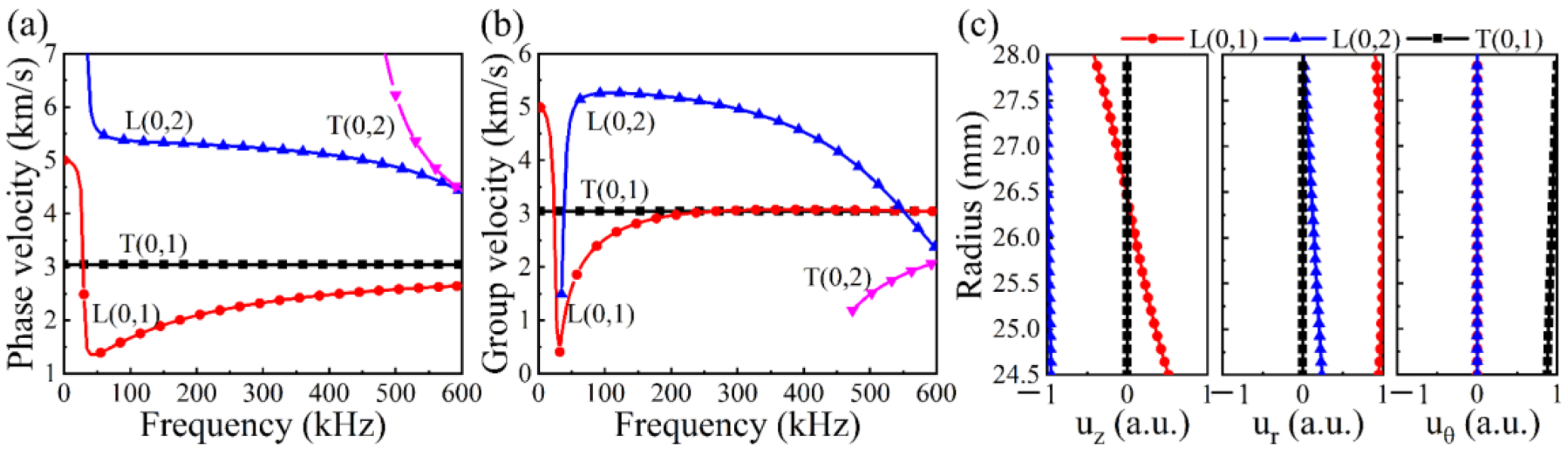
At the aim of reducing the interpretation complexity of UGW signals, it is popular to utilize axisymmetric UGWs (longitudinal L(0,m) and torsional T(0,m)) in their non-dispersive frequency bands instead of non-axisymmetric UGWs (flexural F (n,m), where n and m denote the circumferential order and mode [7]). Two inherent characteristics of dispersion and multi-mode in UGW are inevitably manifested as the UGW velocity varies with the frequency, and as multiple modes of UGWs exist at a given frequency [8,9]. In this context, it is almost impossible to excite the pure UGW at the desired mode, whilst UGWs at undesired modes may be excited for imperfect experimental conditions and multi-mode characteristics. In addition, for the mode conversion caused by the interaction between non-axisymmetric defects and UGWs, dispersive flexural UGWs may arise, which may increase the interpretation complexity and further weaken the ability of defects detection [10,11].

In order to enhance the defect identification and classification of UGW testing, several signal processing methods based on time-frequency analysis have been introduced, including Winger–Ville distribution [12], Hilbert–Huang transform [13], wavelet transform [14], and Chirplet transform [15]. However, the improvement of UGW signal resolution processed by the above methods is limited, and more effective signal processing methods need to be found. At present, signal processing methods aimed at improving the signal-to-noise ratio (SNR) of UGW signals are mainly through separation and elimination of dispersive UGWs; the former is typically represented by matching pursuit (MP) [9,16], and the latter includes dispersion compensation (DC) [17,18], pulse compression (PuC) [19,20], and split spectrum processing (SSP) [10,21]. MP is a sparse approximation algorithm, which is based on the construction of an appropriate over-complete and redundant dictionary and finding the best matching of UGW signals in the dictionary. Although MP can separate overlapping UGWs at different modes, the processing results are highly dependent on the quality of the constructed dictionary, which is accompanied by high computational complexity [22]. DC is another signal processing method commonly applied in UGW testing, where the dispersive UGWs can be eliminated by reversing the effect of dispersion and multi-mode on the desired UGW in the time/space domain, and it can be utilized in combination with PuC [17,18]. Yucel et al. [20] applied DC and PuC to improve the SNR of UGW signals of aluminum rods. Toiyama et al. [23] proposed a method combining PuC and velocity DC in the wave-number domain to compensate for the wave distortion caused by dispersion, and the results showed that the time resolution and SNR of UGW signals were improved. However, DC and PuC need the prior knowledge of dispersion and pipeline structure, which is usually not available in the UGW testing of long-distance pipelines and unknown pipeline structures [24].

SSP can split multi-mode UGWs by separating the received signal into a sub-signal group in the frequency domain and recombining them in the time domain without the knowledge of dispersion and propagation distance [10,21]. SSP was first applied to ground search radar operation [25] and later to conventional ultrasonic detection [26] to reduce the scattering effect of coarse crystals and improve the signal-to-noise ratio. It is rarely applied in the field of UGW testing, there are only a few studies on SSP processing of T(0,1) UGW signals, whereas the studies about the SSP processing of L(0,2) UGW signals cannot be found to the best of the authors’ knowledge. Pedram et al. [10,21,27] applied T(0,1) UGW testing to a coated pipeline; SSP was used to eliminate the noise and improve the SNR, and determined the SSP filter parameters by brute force search method. However, the processing effect of SSP is directly related to the SNR of unprocessed UGW signals, namely high noise levels are harmful to the processing effect, and some defects may not be identified when SSP processes multi-defected UGW signals.

In order to compensate the shortcomings of SSP, this paper proposed an improved SSP (ISSP) based on the raised cosine filter bank with varying bandwidth and spacing, and applied variational mode decomposition (VMD) and wavelet transform (WT) to UGW signals before ISSP. The structure of this paper is as follows: the characteristics of UGWs were analyzed (Section 2); signal processing methods used were introduced (Section 3); SSP was improved by filter bank design, and the pros and cons of ISSP were analyzed (Section 4); signal processing method based on VMD, WT, and ISSP (VWISSP) was proposed to process the UGW signals with noise and multi-defects (Section 5); L(0,2) UGW testing was performed on aluminum and low carbon steel pipes containing different types and numbers of defects, and the processing effect of VWISSP was evaluated (Section 6); and Section 7 is the conclusion.

2. Ultrasonic Guided Wave Characteristics

Guided waves are elastic waves generated directly in the waveguide, which propagate along its length, confined by the geometric limits of its walls [28]. Hence, they propagate through the waveguide and are reflected due to variations in the wall. Before the UGW signals are processed, it is beneficial to have a deeper understanding of UGW characteristics.

2.1. Axisymmetric Ultrasonic Guided Waves

Outer diameter, wall thickness, and the material of the pipe are the factors that influence dispersion, which should be input in advance before PC_disp programs [29] are run. An aluminum pipe with an outer diameter of 56 mm, a wall thickness of 3.5 mm, and a length of 4 m was used, for which the dispersion curves of axisymmetric UGWs were drawn in Figure 1. It can be observed from Figure 1a,b that L(0,1), L(0,2), T(0,1), and T(0,2) UGWs exist in the frequency range of 0 to 600 kHz, and the propagation velocities of UGWs (except T(0,1) UGW) are dependent on frequency, namely dispersion. However, there are specific non-dispersive frequency bands where the propagation velocities of UGWs change little as frequency varies, and it can be noticed that the non-dispersive frequency band of L(0,2) UGW is 90–150 kHz.

UGWs manifest different sensitivities to defects under the relationship between UGW propagation directions and defect distributions, where L(0,2), L(0,1), and T(0,1) UGWs are dominated by axial, radial, and circumferential displacements (Figure 1c). In this way, L(0,2) UGW is mostly suitable for circumferential defect detection. In consideration of UGW testing efficiency, dispersion, and energy attenuation comprehensively, fast-speed L(0,2) UGW with the non-dispersive excitation frequency of 100 kHz was determined, and the corresponding phase and group velocities were 5.372 km/s and 5.261 km/s, respectively.

2.2. Non-Axisymmetric Ultrasonic Guided Waves

In order to ensure the high time-domain resolution of UGW signals, the sinusoidal signals modulated by the Hanning window are the mainstream choice of excitation signals, and the 100 kHz sinusoidal signal modulated by 10 cycles was selected as the excitation signal in this paper, which can be expressed as [10,11]:

$$x_{ex}=\frac{1}{2}\left[1-\cos \left(\frac{2\pi f_{c}t}{n}\right)\right]\sin \left(2\pi f_{c}t\right)$$

(1)

where f_c is the excitation center frequency, t is the time, and n is the Hanning window period. The excitation signals in time and frequency domains are illustrated in Figure 2a, and only L(0,1), L(0,2), and T(0,1) UGWs could be excited in the excitation frequency band (~70–130 kHz). It is worth noting that the excitation conditions of torsional UGWs are completely different from those of longitudinal UGWs, so L(0,1) and L(0,2) UGWs are the most likely to be excited in the excitation frequency band.

The dispersion curves of non-axisymmetric UGWs are shown in Figure 2b,c, where the black curve and gray area denote the spectrum of the excitation signal and frequency band. With the increase of circumferential order n, the phase velocities of F(n,1) and F(n,3) UGWs increase gradually and the group velocities decrease, whilst the velocity difference between F(n,3) and L(0,2) UGWs is much larger compared with that between F(n,1) and L(0,1) UGWs, indicating that F(n,3) is likely to be easily distinguished from L(0,2) while F(n,1) may be overlapped with L(0,1). In this context, F(4,3) and F(5,3) UGWs may not be converted from L(0,2) UGW as their cutoff frequencies are beyond the excitation frequency range.

3. Ultrasonic Guided Wave Signal Processing Methods

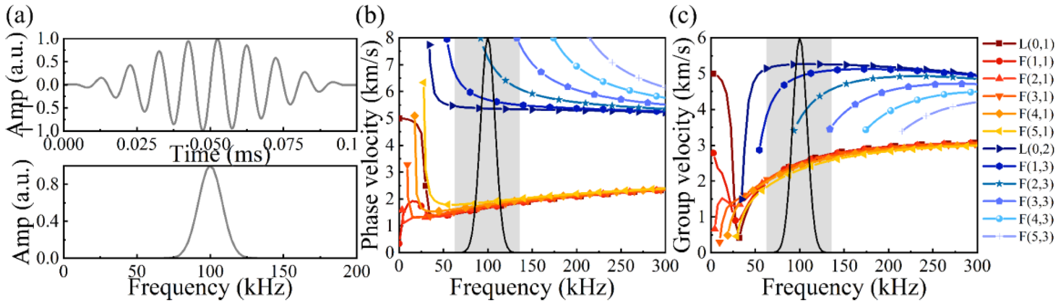
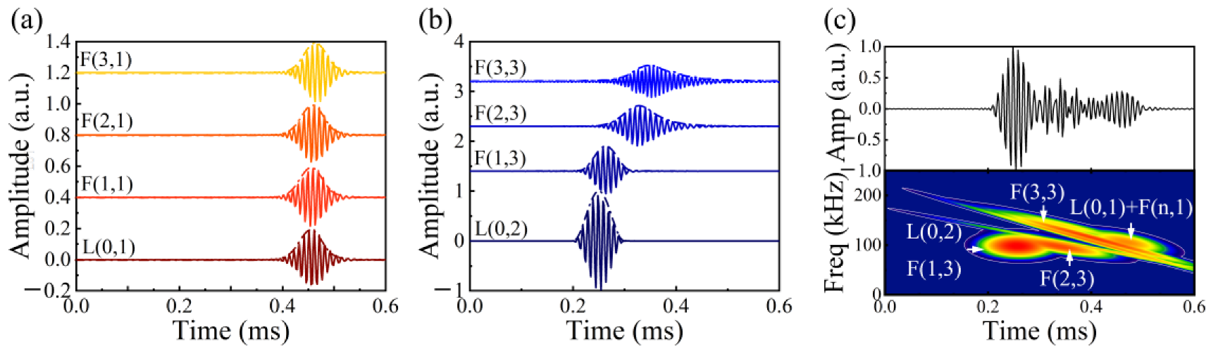
On the basis of UGW characteristics analysis, both undesired L(0,1) and desired L(0,2) UGWs could be excited, and they may be converted to coherent noise (F(n,1) and F(n,3) UGWs) for the interaction between non-axisymmetric defects and UGWs, and incoherent noise caused by the environment and instruments that are likely to interfere with UGW signals. It is beneficial for the accurate identification and location of defects to eliminate noise and retaining feature (defects and pipe end) signals, which can be realized by the following signal processing methods.

3.1. Split Spectrum Processing

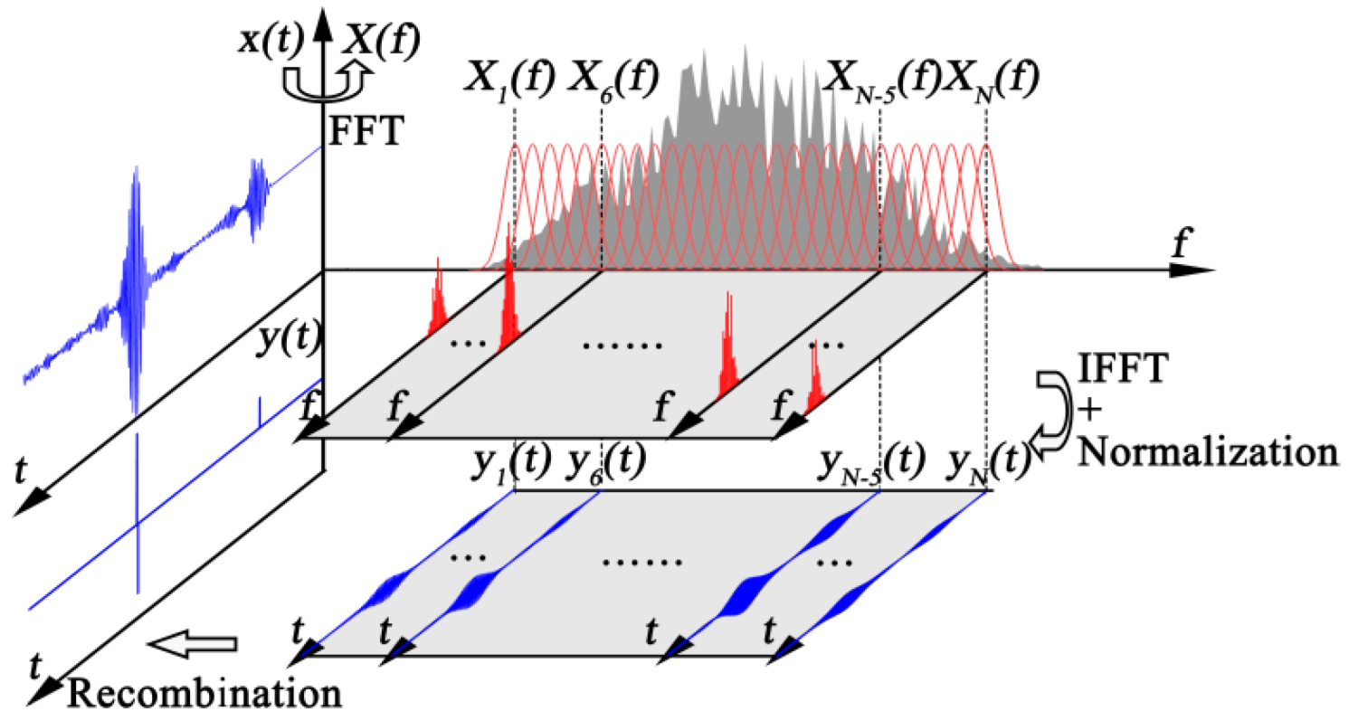
SSP is sensitive to the different frequencies of UGWs at the desired and other modes, that is, the processed sub-band signal group contains the desired mode UGW with a similar amplitude and other mode UGWs with different amplitudes [10,21,27]. The schematic diagram of SSP (Figure 3) can be described as follows. First, the fast Fourier transform (FFT) is applied to transform an input signal x(t) in the time domain into a frequency-domain signal X(f), which is split into a sub-band signal group X_i(f) (i = 1,2,…,N; where N denotes the number of filters) in the frequency domain by an intersecting bandpass filter bank. Then, the inverse FFT (IFFT) on X_i(f) is employed and normalized to obtain a time-domain sub-band signal group y_i(t). Finally, the nonlinear signal recombination methods are utilized to produce an output signal y(t).

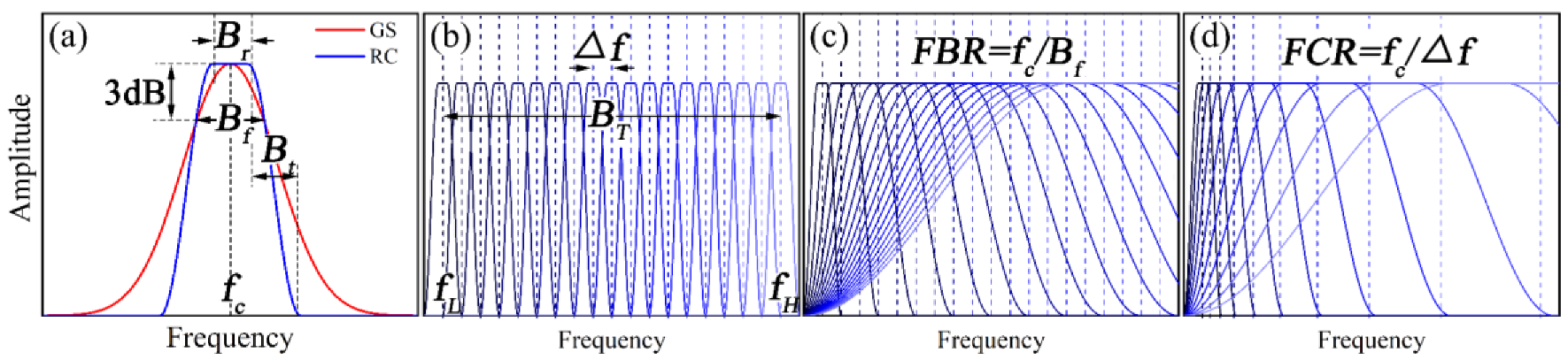
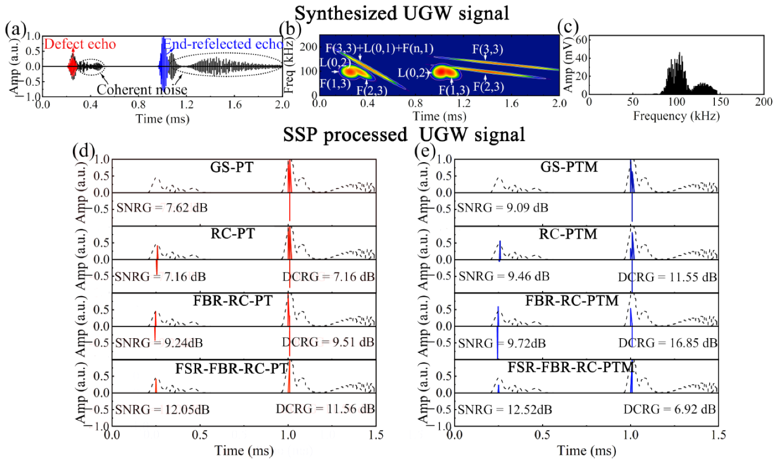
The processing effect of SSP is closely connected with the filter band design, filter band parameters, and signal recombination method, of which the first two will be discussed in Section 4.1. The signal recombination methods considered of SSP are primarily based on order statistics and phase observation [30], which includes normalized minimization, mean, frequency multiplication, polarity thresholding (PT), and polarity thresholding with minimization (PTM). In the light of our previous research [31], the high resolution of sparse signals recombined by PT and PTM is likely to be obtained. PT can be expressed as:

$$\begin{array}{l}{y}_{PT}\left(t\right)=\left\{\begin{array}{ll}x\left(t\right)& if{y}_i\left(t\right)<0or>0,\forall i\\ 0& otherwise\end{array}\right.\end{array}$$

(2)

PTM is similar with PT in form, which also requires that y(t) to take value (min |y_i(t)|) only when the positivity and negativity of all sub-band signals at a certain time are consistent; otherwise, it is zero. Both PT and PTM can eliminate the coherent noise that is highly sensitive to the frequency, which is that the amplitude of the sparse signal recombined by PTM may be distorted, resulting in the inaccurate quantitative analysis results of defects.

3.2. Variational Mode Decomposition

Variational mode decomposition (VMD) can separate harmonic signals with a relatively close frequency range without affecting the sampling frequency, and improve signal SNR by eliminating incoherent noise [32]. Compared with empirical mode decomposition (EMD), VMD has complete mathematical theory, which is more robust to sampling and noise, and shows better decomposition effect on complex non-stationary signals [33]. In VMD, inherent mode functions (IMFs) are defined as AM-FM signals, which are expressed as [34]:

$$u_k\left(t\right)=A_k\left(t\right)\cos \left[{\varphi }_k\left(t\right)\right]$$

(3)

where A_k(t) is the instantaneous non-negative amplitude, φ_k(t) is the undiminished phase function, namely the instantaneous frequency ${\omega }_k\left(t\right)=d{\varphi }_k\left(t\right)/dt\ge 0$.

The VMD model is expressed as follows [35]:

$$\underset{\left\{u_k\right\},\left\{{\omega }_k\right\}}{\min }\left\{{\displaystyle \sum _k{‖{\partial }_t\left[\left(\delta \left(t\right)+\frac{j}{\pi t}\right)\ast u_k\left(t\right)\right]e^{-j{w}_{k}t}‖}_2^2}\right\}$$

(4)

$$s.t.{\displaystyle \sum _k{u}_k}=x$$

(5)

where k is the number of modes, $\left\{u_k\right\}$ and $\left\{{\omega }_k\right\}$ are the kth IMF and the center frequency after decomposition, $\delta \left(t\right)$ is the Dirac delta function, and $\ast$ is the symbol of convolution operation. The VMD process (Algorithm 1) can be concluded as follows: [33,34].

Algorithm 1 VMD

$\mathrm{Initialize}\left\{{\widehat{u}}_k^1\right\}$, $\left\{{\omega }_k^1\right\}$, ${\widehat{\lambda }}^1$, $n\leftarrow 0$

repeat

$n\leftarrow n+1$

for$k=1:K$do

Update ${\widehat{u}}_k^{}$ for all $\omega \ge 0$  ${\widehat{u}}_k^{n+1}\left(\omega \right)\leftarrow \left[\widehat{x}\left(\omega \right)-{\displaystyle \sum _{i\ne k}{\widehat{u}}_i\left(\omega \right)}+\widehat{\lambda }\left(\omega \right)/2\right]/\left[1+2\alpha {\left(\omega -{\omega }_k\right)}^2\right]$

Update ${\omega }_k^{}$  ${\omega }_k^{n+1}\leftarrow {\displaystyle {\int }_0^{\infty }\omega {\left|{\widehat{u}}_k\left(\omega \right)\right|}^{2}d\omega }/{\displaystyle {\int }_0^{\infty }{\left|{\widehat{u}}_k\left(\omega \right)\right|}^{2}d\omega }$

end for

Dual ascent for all $\omega \ge 0$  ${\widehat{\lambda }}^{n+1}\left(\omega \right)\leftarrow {\widehat{\lambda }}^n\left(\omega \right)+\gamma \left[\widehat{x}\left(\omega \right)-{\displaystyle \sum _k{\widehat{u}}_k^{n+1}\left(\omega \right)}\right]$

until convergence ${\displaystyle \sum _k{‖{\widehat{u}}_k^{n+1}-{\widehat{u}}_k^n‖}_2^2/{‖{\widehat{u}}_k^n‖}_2^2}\le \epsilon$

where ${\widehat{u}}_k^{n+1}\left(\omega \right)$, and $\widehat{\lambda }\left(\omega \right)$ are the frequency domain representations of the kth IMF $u_k^{n+1}\left(t\right)$ signal to be decomposed to $x\left(t\right)$ and the Lagrange operator $\lambda \left(t\right)$, respectively, $\alpha$ is the penalty factor, and $\gamma$ is the noise tolerance, which are artificially set.

When the number of modes K is set, the correct mode center frequency ${\omega }_k$ may not be obtained due to the narrow bandwidth of IMF caused by large $\alpha$, while low $\alpha$ could lead to the incoherent noise having a higher level in IMF. The Lagrangian operator is directly affected by $\gamma$, which can enhance the convergence performance in the case of low noise and should be zero in the case of high noise.

3.3. Wavelet Transform

By adding window functions of different widths to the signal (wavelet transform (WT) applies a wider window function to observe the low frequency and a narrower window function to observe the high frequency), wavelet coefficients are obtained, and the signal can then be reconstructed by these coefficients [36]. The wavelet coefficient can be calculated as follows:

$$W=\frac{1}{\sqrt{S}}{\displaystyle \underset{-\infty }{\overset{\infty }{\int }}x\left(t\right)\psi \left(\frac{t-L}{S}\right)}dt$$

(6)

where, S and L are the scaling and translation factors, and $\psi \left(t\right)$ is the mother wavelet functions.

By selecting an appropriate threshold T, wavelet coefficients larger than the threshold are considered to be generated by useful feature signals and should be retained, while wavelet coefficients smaller than the threshold are considered to be generated by useless noise signals and are set to zero [37]. The new wavelet coefficients obtained by thresholding are:

$$W_{new}=\mathrm{sgn}\left(W\right){\left(\left|W\right|-T\right)}_{+}$$

(7)

3.4. Chirplet Transform

As a generalization of wavelet transform and short-time Fourier transform, Chirplet transform can extract signal components with a specific instantaneous frequency and group delay, and overcome the shortcomings of conventional time–frequency representation solutions, such as short-time Fourier transform and Wigner–Ville distribution, that may not achieve good UGW mode separation results. The standard definition of the Chirplet transform is given by the inner product of a basis function g(t) and the signal x(t) [38]:

$$CT=〈x(t),g(t)〉={\displaystyle {\int }_{-\infty }^{\infty }x(t)}{g}^{*}(t)dt$$

(8)

$$g(t)=T_{t0}{F}_{w0}{S}_s{Q}_q{P}_{p}c(t)$$

(9)

where * denotes the complex conjugate, g(t) is the basic function and the Fourier transform of the basic function, T_t0, F_ω0, S_s, Q_q, and P_p are the time shift, frequency shift, scaling, frequency shear, and time shear operators, respectively, and c(t) is one of the chirp signal family.

4. Improved Split Spectrum Processing

At present, the research of SSP mainly includes filter bank design, filter parameters optimization and signal recombination methods. Since SSP is very sensitive to filter parameters (total bandwidth, filter bandwidth, and filter spacing), the identical optimal filter parameters corresponding to UGW signals may not be determined, of which brute force search method was introduced [10]. The signal recombination methods have been analyzed in Section 3.1, so the improvement for SSP in this paper is aimed at the design of filter bank.

4.1. Filter Bank Design

Gaussian bandpass filters are commonly used in SSP for the ease of implementation. On the one hand, the non-overlapping filters should be evitable for the “picket fence” effect wherein substantial feature information would be lost, which is not conducive to the signal interpretation. On the other hand, the overlapping region of adjacent filters should be controlled to be as small as possible for better coherent noise elimination [39]. Hence, the filter bank design should take into account the above requirements.

In addition to Gaussian (GS) filters, raised cosine (RC) filters can also be an alternative (Figure 4a), who’s transition bands are in the shape of truncated raised cosine cycle, and that guarantee the energy contained is mostly concentrated around the center frequency (the flat top) [40]. Given the same filter spacing, it is easy to foresee that RC filters have better effects on eliminating coherent noise and splitting substantial feature signals, considering that the overlapping of RC filters is lower than that of GS filters.

The filter parameters shared by GS and RC filters are total bandwidth B_T, filter bandwidth B_{f ,} and filter spacing Δf, of which B_T is the difference between high f_H and low f_L cut-off frequencies, and B_fRC can be replaced by the transition bandwidth B_t and the flat top width of B_r. On the premise of eliminating coherent noise and extracting feature signals, the filters with small bandwidths would be the unavoidable choice, which may lead to the poor time resolution of the processed signal. In view of the above problem, this paper adopts the RC filters with variable bandwidths of which the ratio of center frequency to filter bandwidth (FBR = f_c/B_f) is constant, and their frequency distributions are shown in Figure 4c. As the center frequency of FBR-RC filters increases, it is beneficial to increase filter spacing in case of large overlapping between adjacent filters, which can be realized by introducing the ratio of center frequency to filter spacing (FSR = f_c/Δf). According to the analysis, FSR-FBR-RC filter bank (Figure 4d) would be the better option, and the SSP using it can be denoted as the improved SSP (ISSP).

4.2. Advantages of ISSP

The synthesized UGW signals can be utilized to illustrate the advantages of ISSP, which were generated by PC_disp package. The synthesized L(0,1), F (n,1), L(0,2) and F(n,3) (1 ≤ n ≤ 3) UGW signals propagating 1 m in the time domain were plotted in Figure 5a and b. Since the group velocities of F(n,1) and F(n,3) UGWs decrease with the increase of n from the analysis in Section 2.2, their arrival times at the same propagation distance are gradually backward. It can be observed that the time-domain differences among L(0,1) and F(n,1) UGWs are quite small compared with that among L(0,2) and F(n,3) UGWs, which can also be explained by the difference of their group velocities. Moreover, F(n,3) UGWs manifest significant dispersion at high n, namely their wave packets become wider and time resolutions weaken. Superimposing the above UGWs in the time domain, and applying Chirplet transformation to the synthesized signal, creates the results shown in Figure 5c. This distinguishes L(0,2) UGW from synthesized signal by the time-frequency domain signal, but the resolution of L(0,2) UGW is inevitably influenced by other UGWs.

In consideration of the real UGW testing, multiplying the amplitude of L(0,1) + F(n,1) + L(0,2)+ F(n,3) synthesized signal at 1 m by 0.5 (the defect echo), setting the L(0,1) + F(n,1) + L(0,2) + F(n,3) synthesized signal at 5 m as the end-reflected echo, and the synthesized UGW signals in time, creates the following time-frequency and frequency domains that are illustrated in Figure 6a–c.

SSP with different filter bands were used to process the synthesized UGW signal, and the results are shown in Figure 6d,e, where the filter parameters are as follows: B_T = B_3dB, B_f = B_T/10, Δf = B_T/20, B_r = B_T/20, B_t = B_T/40, FBR = f_L/(B_r + 2B_t), FSR = f_L/Δf₀ (Δf₀ = B/20). The signal-to-noise ratio gain (SNRG) and defect-to-noise ratio gain (DNRG) are introduced to quantitatively measure the effects of SSPs, and their calculation formulas are as follows:

$$SNRG=20\left[{\log }_{10}\left(S_{out}/N_{out}\right)-{\log }_{10}\left(S_{in}/N_{in}\right)\right]$$

(10)

$$DNRG=20\left[{\log }_{10}\left(D_{out}/N_{out}\right)-{\log }_{10}\left(D_{in}/N_{in}\right)\right]$$

(11)

where S is the maximum amplitude of the signal, D is the amplitude of the defect echo, N is the noise level calculated by the root mean square of the whole signal, and subscripts in and out represent before and after the SSP processing, respectively.

Compared with the synthesized UGW signal, the sparse signals after applying SSPs show the features (defect and pipe end) obviously, and the coherent noise is successfully eliminated (Figure 6d,e). It can be observed that GS-SSP only retains the end-reflected echo while the defect echo vanishes, and RC-SSP completely retains both. Compared with RC-SSP, FBR-RC-SSP and FSR-FBR-RC-SSP further improve the signal resolution, of which SNRG increases by 29.05% and 68.29%, and DNRG increases by 32.81% and 61.45%, respectively, when PT is taken as the signal recombination method. Despite the enhancement of SNRG and DNRG, the likelihood of amplitude distortion by PTM should be avoided.

4.3. Disadvantages of ISSP

Although ISSP can improve the resolution of UGW signal by eliminating coherent noise and preserving feature signals, there are still some disadvantages of ISSP: (1) ISSP is sensitive to noise level, that is, the SNR of pre-processing UGW signal before should not be too low; (2) ISSP may fail to recognize all defects in dealing with multi-defect UGW signal.

The synthesized UGW signal containing defects in Section 4.2 is denoted as PUS 1 (pure UGW signal 1), and the noisy UGW signals (NUSs) composed of PUS 1 and Gaussian noise (incoherent noise) of different power (0.25 to 6.25 × 10⁻² W) were plotted in Figure 7a, and the sparse signals processed by ISSP-PT and ISSP-PTM are shown in Figure 7b,c. D1 and END represent defect 1 and pipe end respectively, the yellow regions denote the pipe features, and the grey regions represent the misjudgments (uneliminated noise and unrecognized features). It can be observed that ISSP still has the capacity of eliminating noise and preserving features at low incoherent noise level (NUS 1–1), but the effects of ISSP weaken as the increase of incoherent noise level, where uneliminated noise interferes with the recognition of defect. It can be found that the defect signal in NUS 1–5 is completely submerged in the noise, and misjudgments of the sparse signal reach the highest, indicating that ISSP fails in this case.

The multi-defect UGW signals were synthesized by superimposing PUS 1 and synthesized UGW signals (L(0,1) + F(n,1) + L(0,2) + F(n,3)) at 2 m, 3 m, and 4 m, namely PUS 2 to 4; NUSs were obtained by the superposition of PUSs and incoherent noise (1.00 × 10⁻² W); both PUSs and NUSs were processed by ISSP; and the above signals are shown in Figure 8. It can be found that the effects of ISSP on PUS and NUS weaken with the increase of the number of defects, of which the effects of ISSP on NUS are much poorer, implying that noise level and number of defects do influence the ISSP. However, there are more misjudgments, it can also be noticed that multiple peaks appeared within a single region (PUS 4 D1, NUS 2 D1), and the peak time of defect signal after ISSP are inconsistent with the actual peak time (PUS 4 D3, NUS 4 D1, NUS 4 D3), which not only confuses the defect discrimination but also harms the accuracy of locating the defect. In addition, PTM may still lead to the amplitude distortion, whilst PT has the ability to reflect the feature signals completely and accurately, so it is reasonable to choose PT as the following signal recombination method.

5. Signal Processing Method based on VMD, WT and ISSP

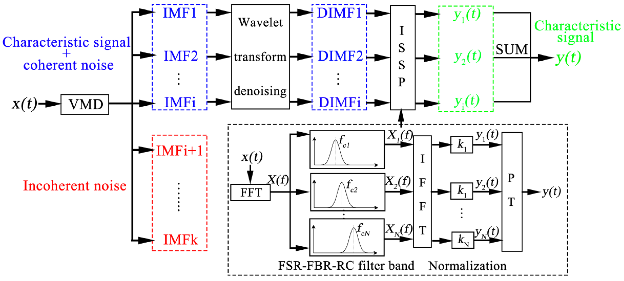
The reason why ISSP may fail in the case of high noise level and multiple defects is related to the low SNR of UGW signal before processing, which can be improved by the denoising function of variational mode decomposition (VMD) and wavelet transform (WT). Therefore, it is promising to combine VMD, WT, and ISSP (VWISSP) to process UGW signals, whose schematic diagram is illustrated in Figure 9. Firstly, the UGW signal x(t) was processed by VMD to obtain the IMFs, which were classified into useful features and useless incoherent noise according to the correlation analysis. Then, the useless IMFs containing incoherent noise are discarded, and the useful IMFs are denoised by WT to obtain DIMFs. Finally, DIMFs are processed by ISSP to obtain y_i(t), which are summed to obtain y(t) containing only feature signals.

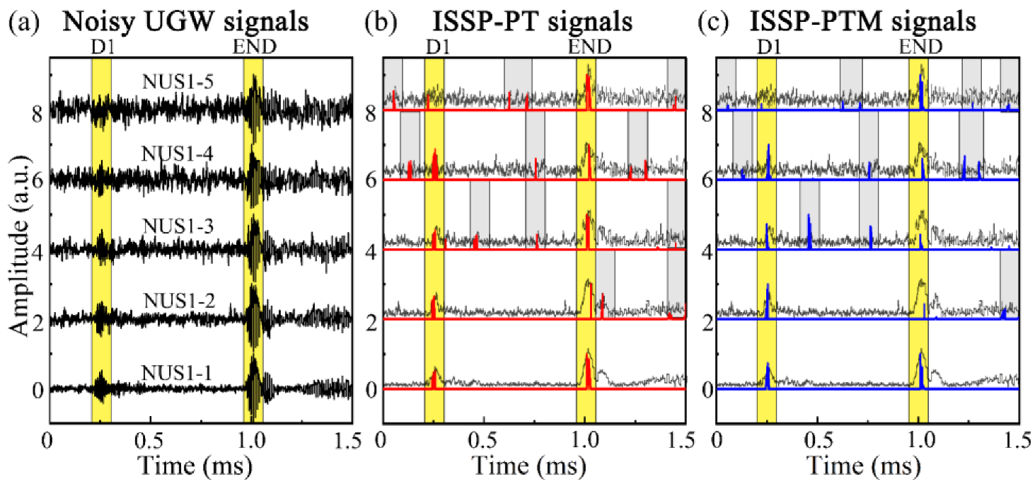
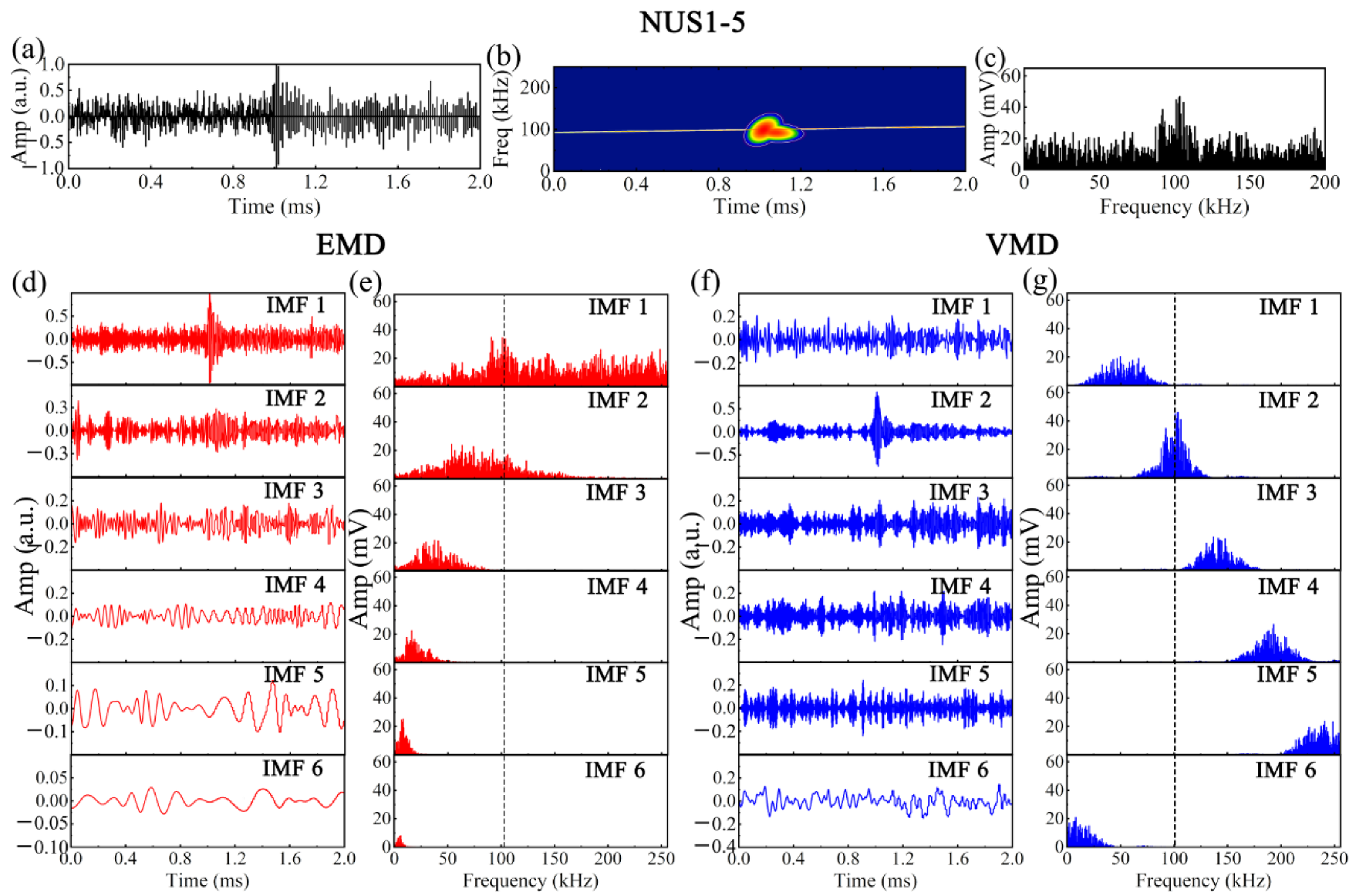
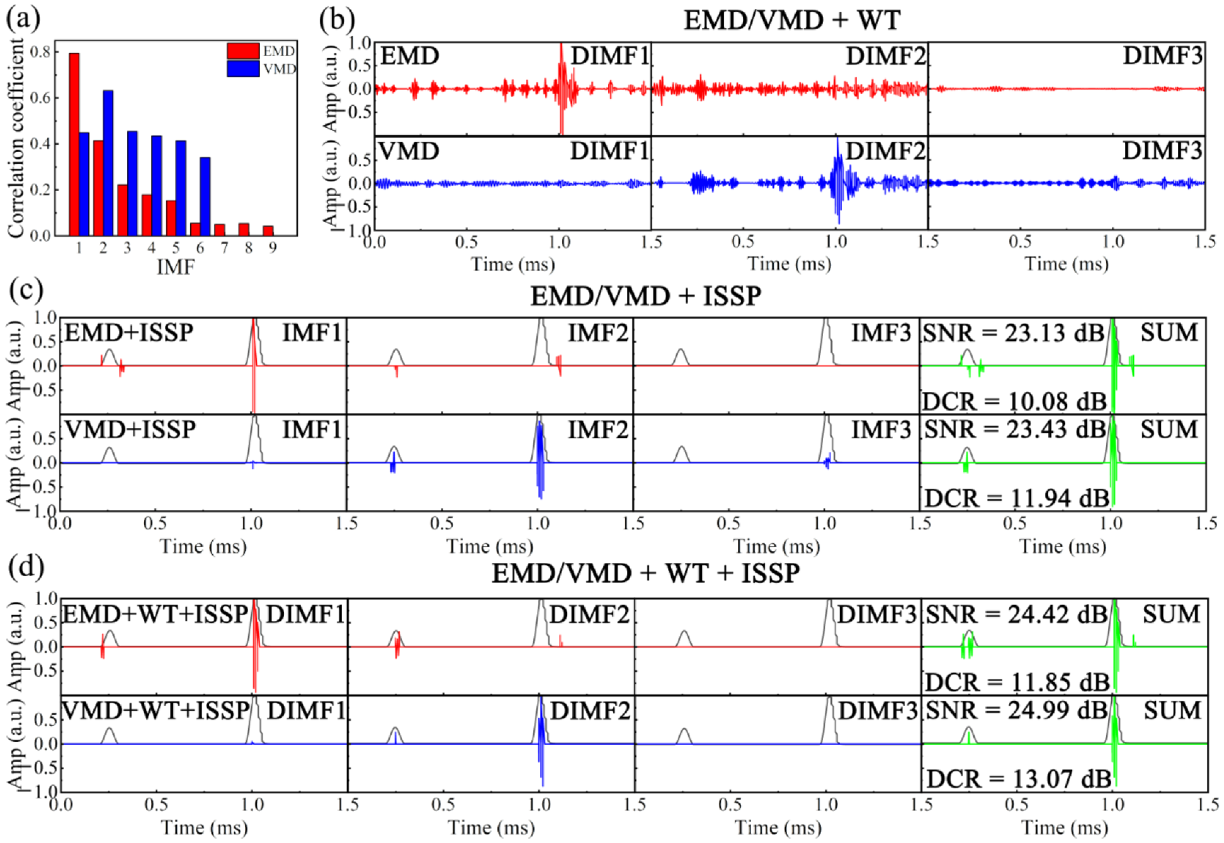
Due to the significant influence of incoherent noise, it is difficult to distinguish the defect signal from the NUS 1–5 in the time and time-frequency domains (Figure 10a,b), while the spectrum may also be polluted (Figure 10c). After performing EMD and VMD on NUS 1–5, the resulting first six IMFs in time and frequency domains are shown in Figure 10d-g, and their correlation coefficients with NUS 1–5 are calculated (Figure 11a). It can be noticed that IMF 1 and IMF 2 of EMD show the highest similarity with NUS 1–5, of which the correlation coefficients are 0.79 and 0.41, and the features in IMF 1 and IMF 2 are the pipe end and the defect, and other IMFs can be considered as having no practical significance. Only IMF 2 with the highest correlation coefficient (0.63) of VMD is concentrated around 100 kHz, indicating that all features can be revealed through IMF 2, and the rest of IMFs can be considered as the incoherent noise.

It can be found from Figure 11b that WT can enhance the resolution of IMFs and the features of DIMFs become more obvious, and the sparse signals of IMFs and DIMFs after applying ISSP are shown in Figure 11c,d. Compared with ISSP, E/VMD + ISSP can significantly reduce the misjudgments and further improve the signal resolution. However, multiple peaks would appear in the defect region processed by EMD + ISSP, which confuses the accurate identification of defects, while VMD + ISSP has no such trouble. Thanks to the denoising of WT, the resolution of sparse signals processed by E/VMD + WT + ISSP are enhanced further, of which SNRs are 24.42 dB and 24.99 dB, and DNRs are 11.85 dB and 13.07 dB.

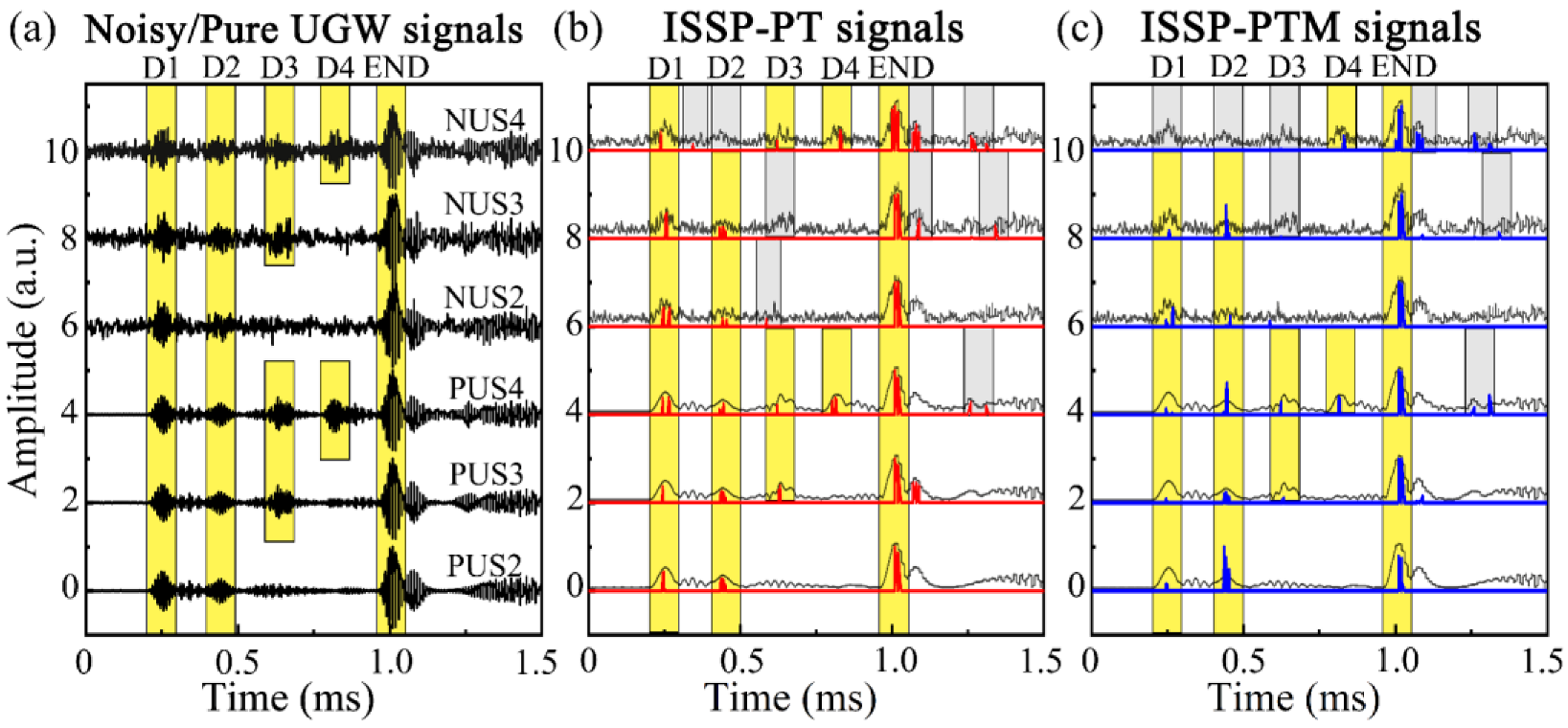
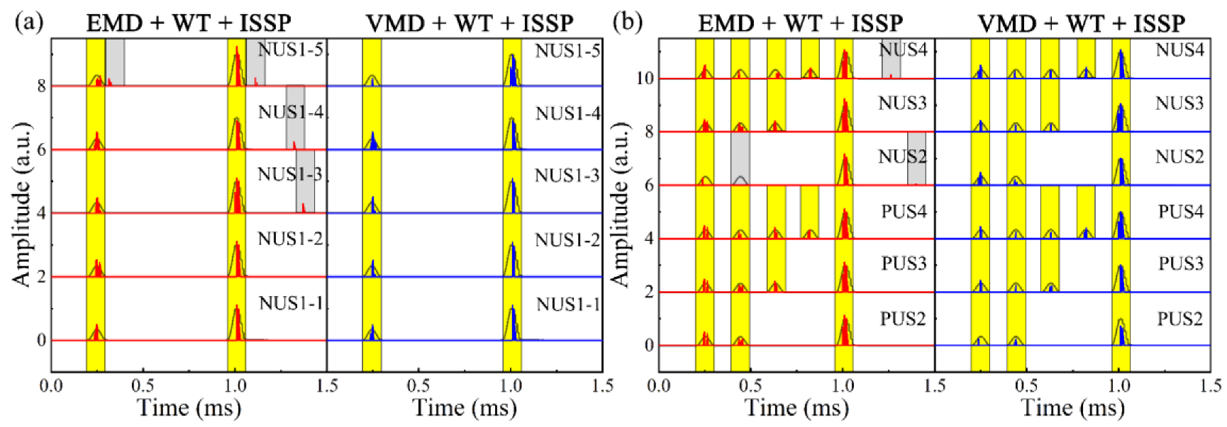
The denoting results of the E/VMD + WT + ISSP as E/VWISSP, which were applied to NUS and PUS in Section 4, are illustrated in Figure 12, and the calculated SNRG, DNRG, and number of misjudgments are shown in

Table 1. SNRG, DNRG, and misjudgments of N/PUS signals processed by ISSP, EWISSP, and VWISSP.

	SNRG(dB)			DNRG(dB)			Misjudgments
	ISSP	EWISSP	VWISSP	ISSP	EWISSP	VWISSP	ISSP	EWISSP	VWISSP
NUS 1–1	7.32	7.73	7.9	6.57	6.67	7.32	0	0	0
NUS 1–2	9.06	8.79	10.48	11.44	8.59	10.07	2	0	0
NUS 1–3	8.83	9.01	11.04	8.83	8.91	10.54	3	1	0
NUS 1–4	7.47	10.54	10.93	7.73	11.53	11.76	4	1	0
NUS 1–5	8.86	12.05	12.48	6.81	8.65	9.43	4	2	0
PUS 2	6.80	7.04	8.53	6.73	7.20	7.81	0	0	0
PUS 3	6.05	6.72	7.61	5.72	6.18	7.12	0	0	0
PUS 4	6.77	7.26	7.57	5.29	7.08	7.10	2	0	0
NUS 2	7.56	8.73	9.67	5.75	5.45	6.84	1	2	0
NUS 3	7.48	8.70	9.46	5.28	5.98	6.22	3	0	0
NUS 4	7.31	8.48	9.49	5.85	7.38	8.34	4	1	0

. Compared with ISSP, EWISSP and VWISSP can further improve the signal resolution, with the average SNRG increased by 13.76% and 25.73%, respectively, and the average DNRG increased by 12.43% and 23.95%, respectively. However, EWISSP cannot retain the features and eliminate noise completely. Therefore, VWISSP based on VMD, WT and ISSP can be considered as the most suitable method to gain the sparse UGW signals with high accuracy and resolution, of which only feature signals are retained and noise signals are eliminated completely.

6. Experiments of Ultrasonic Guided Wave Testing

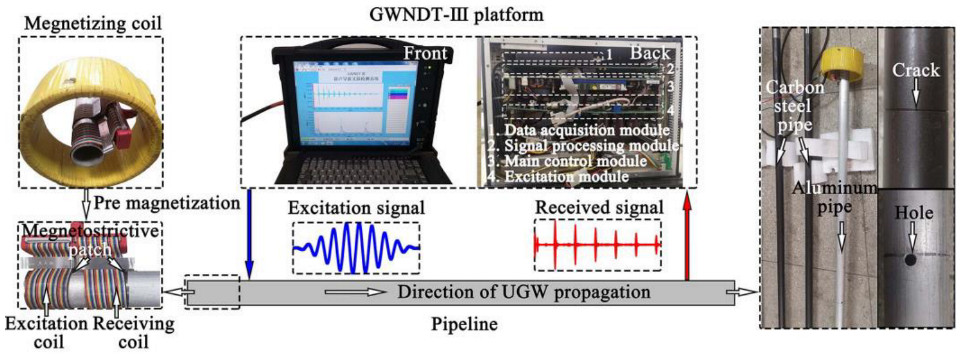
UGWs can be excited and received based on the principles including, but not limited to, magnetostriction, piezoelectricity, and electromagnetism. Magnetostrictive UGW testing was chosen for the ease of implementation, low cost, and excellent sensitivity and durability, of which the schematic diagram is shown in Figure 13. The magnetostrictive UGW testing system includes a self-made GWNDT-III platform, magnetizing coil, magnetostrictive patch (FeCo alloy), excitation/receiving coils and pipe; and the GWNDT-III platform integrates the modules of main control, excitation, data acquisition, and signal processing, which can realize the excitation and reception of UGW conveniently.

The principle of magnetostrictive UGW testing is as follows [41]. Firstly, ensure that the magnetostrictive patch is in a state of maximum magnetostriction rate pre-magnetizing the magnetization coil. Secondly, excite the excitation signal using the GWNDT-III platform, which generates dynamic magnetostriction in the form of UGW based on positive magnetostrictive effect. Finally, the induced voltage signal of the receiving coil resulting from the variation of magnetic field strength near the magnetostrictive patch based on the inverse magnetostrictive effect can be captured, which is processed and exhibited by the GWNDT-III platform.

6.1. Aluminum Pipe

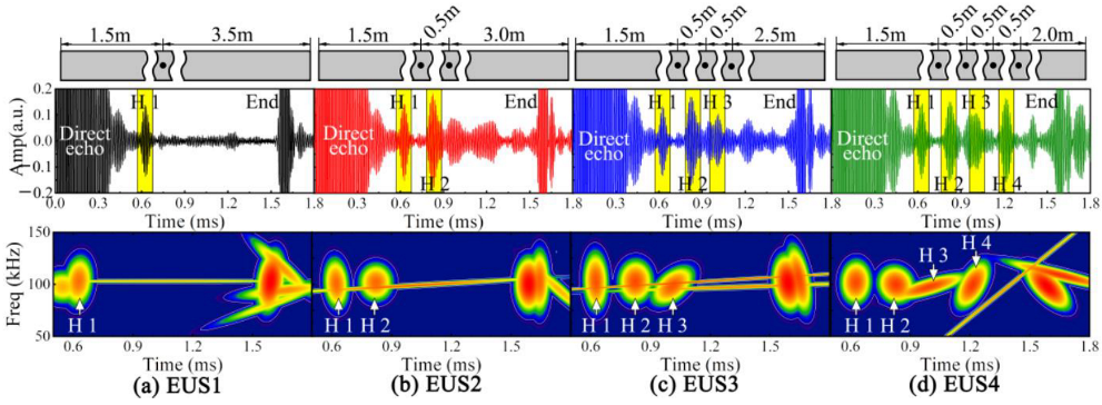
The hole defects (H1, H2, H3, and H4) with diameters of 10 mm were artificially set on the surface of the aluminum pipe, of which their axial positions are illustrated in the upper Figure 14, and the L(0,2) UGW testing signals for the above aluminum pipes are shown in the middle Figure 14. It can be observed that UGW signals mainly comprise of direct echo, defect echo, end-reflected echo, and noise signal (coherent and incoherent noise). With the increase of the number of defects, the noise level, especially the coherent noise level, increases significantly, which can be attributed to the reflection, refraction, and mode conversion of UGWs, and it can be found that the defect resolution becomes poor in EUS 3 and 4. Removing the direct echo that is seriously affected by electromagnetic radiation, and applying the Chirplet transform to the residual signals, creates the results shown in the bottom Figure 14. Although Chirplet transform shows the defects clearly in time-frequency domain, the accurate localization of defects may not be achieved due to the interference of noise.

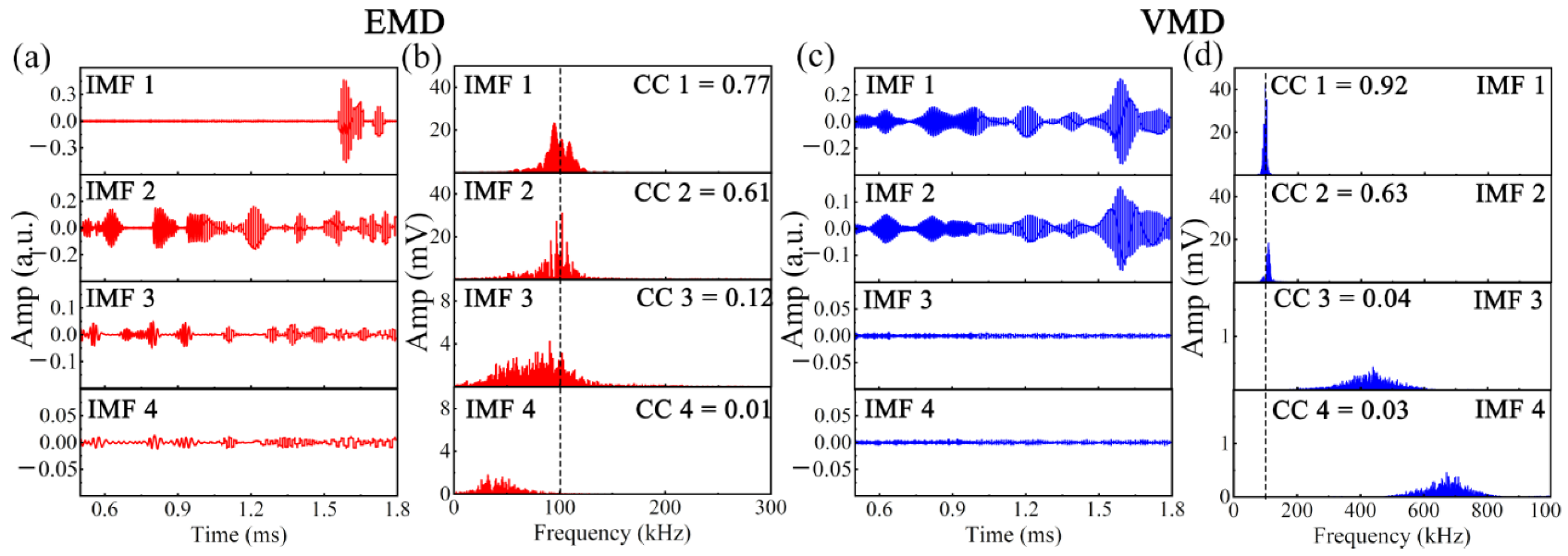
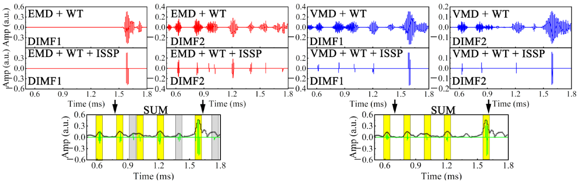
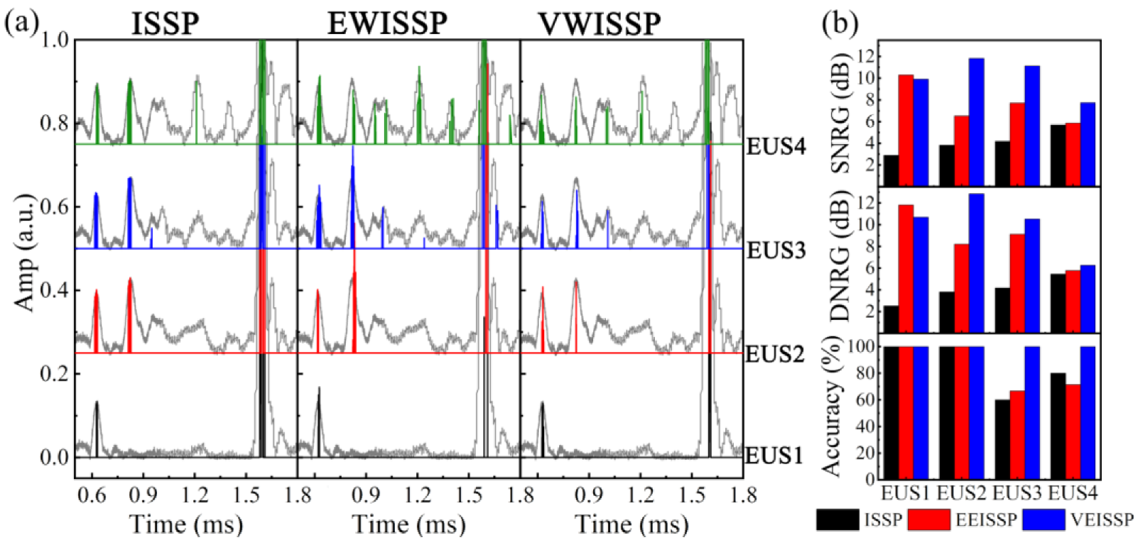
The first four IMFs of EUS 4 were gained by EMD and VMD, which are shown in Figure 15. It can be found that the first two IMFs of EMD and VMD show high similarity with EUS 4, and it can be considered that the IMF 1 and IMF 2 of EMD contain the features of pipe end and defect, respectively, and both the IMF 1 and IMF 2 of VMD contain all features. Figure 16 shows the results after discarding the meaningless IMFs of EMD and useless IMFs (incoherent noise) of VMD, performing WT on the substantial IMFs (IMF 1 and 2) to get DIMFs, and applying the ISSP to the DIMFs. It can be seen that VWISSP can completely retain the features and eliminate the noise, thus realizing the high accuracy and resolution processing of the UGW signal, while EWISSP may mistakenly retain the coherent noise as the features.

ISSP, EWISSP and VWISSP were used to process EUS 1 to 4, and the SNRGs, DNRGs and accuracies of the processed sparse signals were calculated, for which the accuracy calculation formula is shown in Equation (12), and the results are shown in Figure 17.

$$Accuracy=\frac{N_F-N_F^U}{N_F-N_F^U+N_M}$$

(12)

where, $N_F$ is the number of features, $N_M$ is the number of misjudgments (the sum of uneliminated noise signals and unrecognized feature signals $N_F^U$).

From the perspective of signal resolution, the higher signal resolution is conducive to the location of pipe features. Therefore, the effect of ISSP is relatively poor, the average SNRG and DNRG are 4.15 dB and 3.99 dB, respectively. The effect of EWISSP is improved, for which the average SNRG and DNRG are 7.60 dB and 8.74 dB, respectively. The effect of VWISSP is the best, for which the average SNRG and DNRG are as high as 10.15 dB and 10.08 dB, respectively. From the perspective of detection accuracy, they can all achieve 100% recognition of pipe features when the defects are few (NUS 1 and 2), but ISSP and EWISSP may miss defect signals or identify noise as defect signals mistakenly if there exists relatively many defects (NUS 3 and 4), which is manifested by a reduction in accuracy from 60% to 80%.

6.2. Low Carbon Steel Pipe

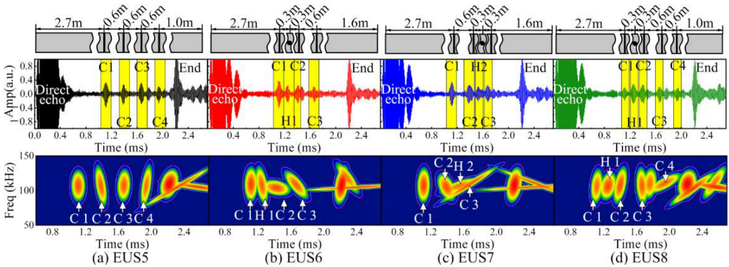
The crack defects (width 2 mm, depth 2 mm, circumferential angle 300°) and hole defects (diameter 10 mm) were artificially set on the surface of a low carbon steel pipe (outer diameter 48 mm, wall thickness 5 mm, length 5.5 m), and their axial positions are illustrated in the upper Figure 18. The L(0,2) UGW signals are shown in the middle of Figure 18. It can be concluded that both time domain analysis and Chirplet transform (bottom Figure 18) would not meet the accurate recognition and localization of defects.

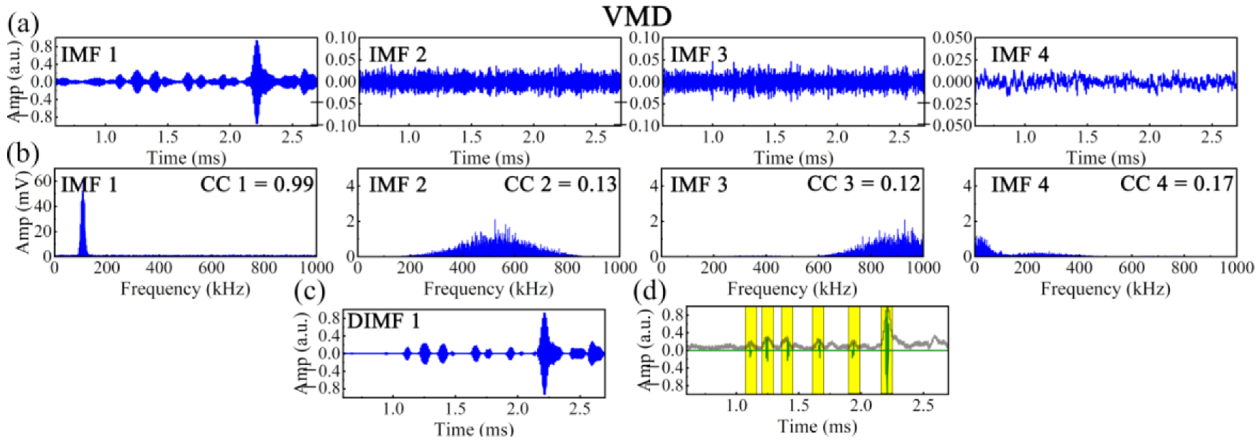
The processing results of VMD, VMD + WT, and VMD + WT + ISSP on EUS 8 are shown in Figure 19. The correlation coefficient of IMF 1 is 0.99, which includes all the feature signals. The correlation coefficient of IMF 2 to 4 is between 0.12 and 0.17, which mainly includes the incoherent noise. The SNR of DIMF 1 is improved by WT denoising by further eliminating noise while preserving the feature signals. After applying ISSP to DIMF 1, there is no noise signal completely in the sparse signal, so the accurate defect recognition and localization can be realized.

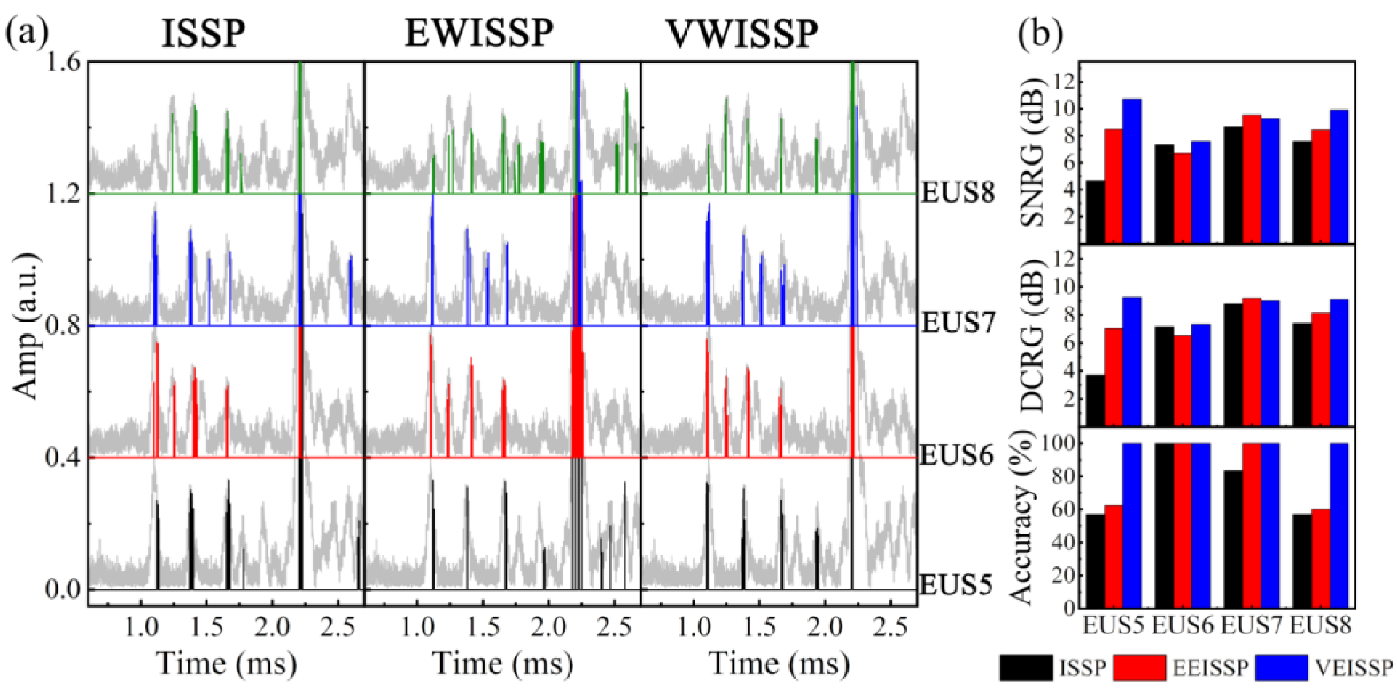
ISSP, EWISSP, and VWISSP were used to process EUS 5 to 8, and the SNRGs, DNRGs and accuracies of the sparse signals were calculated, and the results are shown in Figure 20. The three methods can be ranked according to the processing effect as follows: VWISS > EWISSP > ISSP. The average SNRG, DNRG, and accuracy of VWISSP are 9.41 dB, 8.68 dB, and 100%, respectively, while the average SNRG, DNRG, and accuracy of ISSP are 7.07 dB, 6.77 dB, and 74.37%, respectively, which are improved by 32.97%, 28.25%, and 34.46%, respectively. To sum up, VWISSP has the promising ability to manifest the feature signals (defect and pipe end) in the form of obviously sparse signals, which solves the problems of the poor processing effect of ISSP on the UGW signals with high noise levels and multiple defects, and realizes the accurate recognition and location of defects.

7. Conclusions

An advanced signal processing method based on variational mode decomposition (VMD), wavelet transform (WT), and improved split spectrum processing (ISSP) was proposed to improve the signal interpretation accuracy of the L(0,2) ultrasonic guided wave (UGW) signals, of which SSP may not achieve great pipe feature preservation on noisy multi-defect UGW signals.

To begin with, it is essential to illustrate the UGW characteristics of dispersion and multi-mode, and UGW signals were divided into signals of features (desired UGW), coherent noise (undesired and non-axisymmetric UGWs), and incoherent noise (environmental noise). SSP was improved by replacing the Gaussian filter bank with cosine filters of constant frequency-to-bandwidth and frequency-to-filter spacing ratios (FSR-FBR-SSP), of which the pros and cons were revealed.

The enhancement effects of VMD and WT on the signal to noise ratio (SNR) were exploited: combining them with ISSP is more beneficial to preserving features (defects and pipe end) and eliminating noise, which is inducive to obtain better signal interpretation accuracy. The L(0,2) UGW testing was performed on aluminum and low carbon steel pipes containing different types and numbers of defects, and the signal processing method based on VMD, WT, and ISSP (VWISSP) was applied on the UGW signals. The signal-to-noise ratio gain (SNRG), defect-to-coherent noise gain (DNRG), and feature accuracy were introduced, and the results illustrated that VWISSP shows better capacity for obtaining the sparse UGW signals with high accuracy and resolution compared with ISSP, of which only feature signals are retained and noise signals are eliminated completely.

References

1. Adegboye, M.A.; Fung, W.K.; Karnik, A. Recent advances in pipeline monitoring and oil leakage detection technologies: Principles and approaches. Sensors 2019, 19, 2548. [Google Scholar] [CrossRef] [PubMed] [Green Version]
2. Olisa, S.C.; Khan, M.A.; Starr, A. Review of current guided wave ultrasonic testing (GWUT) limitations and future directions. Sensors 2021, 21, 811–818. [Google Scholar] [CrossRef] [PubMed]
3. Ling, E.H.; Abdul Rahim, R.H. A review on ultrasonic guided wave technology. Aust. J. Mech. Eng. 2020, 18, 32–44. [Google Scholar] [CrossRef]
4. Ghavamian, A.; Mustapha, F.; Baharudin, B.; Yidris, N. Detection, localisation and assessment of defects in pipes using guided wave techniques: A review. Sensors 2018, 18, 4470. [Google Scholar] [CrossRef] [PubMed] [Green Version]
5. Wang, Y.M.; Yang, B. Theory and Method of Magnetostrictive Guided Wave Nondestructive Testing; Science Press: Beijing, China, 2015. [Google Scholar]
6. Guan, R.; Lu, Y.; Duan, W.; Wang, X. Guided waves for damage identification in pipeline structures: A review. Struct. Control Health Monit. 2017, 24, e2007. [Google Scholar] [CrossRef]
7. Narayanan, M.M.; Arjun, V.; Kumar, A.; Mukhopadhyay, C.K. Development of In-bore Magnetostrictive Transducer for Ultrasonic Guided Wave based-inspection of Steam Generator Tubes of PFBR. Ultrasonics 2020, 106, 106148. [Google Scholar] [CrossRef]
8. Nakhli Mahal, H.; Yang, K.; Nandi, A.K. Defect detection using power spectrum of torsional waves in guided-wave inspection of pipelines. Appl. Sci. 2019, 9, 1449. [Google Scholar] [CrossRef] [Green Version]
9. Rostami, J.; Tse, P.W.T.; Fang, Z. Sparse and dispersion-based matching pursuit for minimizing the dispersion effect occurring when using guided wave for pipe inspection. Materials 2017, 10, 622. [Google Scholar] [CrossRef] [Green Version]
10. Pedram, S.K.; Fateri, S.; Gan, L.; Haig, A.; Thornicroft, K. Split-spectrum processing technique for SNR enhancement of ultrasonic guided wave. Ultrasonics 2018, 83, 48–59. [Google Scholar] [CrossRef]
11. Malo, S.; Fateri, S.; Livadas, M.; Mares, C.; Gan, T.H. Wave mode discrimination of coded ultrasonic guided waves using two-dimensional compressed pulse analysis. IEEE Trans. Ultrason. Ferroelectr. Freq. Control 2017, 64, 1092–1101. [Google Scholar] [CrossRef]
12. Wu, J.; Chen, X.; Ma, Z. A signal decomposition method for ultrasonic guided wave generated from debonding combining smoothed pseudo Wigner-Ville distribution and Vold–Kalman filter order tracking. Shock Vib. 2017, 7283450. [Google Scholar] [CrossRef] [Green Version]
13. Cao, H.; Jiang, M.; Jia, L.; Ma, m.; Sun, L.; Zhang, L.; Tian, A.; Liang, J. An ultrasonic signal processing method to improve defect depth estimation in composites based on empirical mode decomposition. Meas. Sci. Technol. 2021, 32, 115112. [Google Scholar] [CrossRef]
14. Muñoz, C.Q.G.; Jiménez, A.A.; Márquez, F.P.G. Wavelet transforms and pattern recognition on ultrasonic guides waves for frozen surface state diagnosis. Renew. Energy 2018, 116, 42–54. [Google Scholar] [CrossRef]
15. Kim, C.Y.; Park, K.J. Mode separation and characterization of torsional guided wave signals reflected from defects using chirplet transform. NDT E Int. 2015, 74, 15–23. [Google Scholar] [CrossRef]
16. Li, C.; Wang, Y.; Zhu, L. Application of improved matching pursuit method in guided wave signal processing. J. Vib. Meas. Diagn. 2012, 32, 111–115. [Google Scholar]
17. Zhao, M.; Wang, H.; Xue, B.; Yue, Y.G.; Zhang, P.F.; Lv, F.Z.; Tang, Z.F. Research on ultrasonic guided wave dispersion compensation for steel strand defect detection. IOP Conf. Ser. Mater. Sci. Eng. 2020, 740, 012101. [Google Scholar] [CrossRef]
18. Luo, Z.; Zeng, L.; Lin, J. A novel time–frequency transform for broadband Lamb waves dispersion characteristics analysis. Struct. Health Monit. 2021, 20, 3056–3074. [Google Scholar] [CrossRef]
19. De Marchi, L.; Perelli, A.; Marzani, A. A signal processing approach to exploit chirp excitation in Lamb wave defect detection and localization procedures. Mech. Syst. Signal Process. 2013, 39, 20–31. [Google Scholar]
20. Yücel, M.K.; Fateri, S.; Legg, M.; Wilkinson, A.; Kappatos, V.; Selcuk, C.; Gan, T.H. Coded waveform excitation for high-resolution ultrasonic guided wave response. IEEE Trans. Ind. Inform. 2015, 12, 257–266. [Google Scholar] [CrossRef]
21. Pedram, S.K.; Haig, A.; Lowe, P.S.; Thornicroft, K.; Gan, L.; Mudge, P. Split-spectrum signal processing for reduction of the effect of dispersive wave modes in long-range ultrasonic testing. Phys. Procedia 2015, 70, 388–392. [Google Scholar]
22. Wang, G.; Wang, Y.; Sun, H.; Miao, B.; Wang, Y. A reference matching-based temperature compensation method for ultrasonic guided wave signals. Sensors 2019, 19, 5174. [Google Scholar] [CrossRef] [Green Version]
23. Toiyama, K.; Hayashi, T. Pulse compression technique considering velocity dispersion of guided wave. AIP Conf. Proc. Am. Inst. Phys. 2008, 975, 587–593. [Google Scholar]
24. Xu, C.B.; Yang, Z.B.; Chen, X.F.; Tian, S.H.; Xie, Y. A guided wave dispersion compensation method based on compressed sensing. Mech. Syst. Signal Process. 2018, 103, 89–104. [Google Scholar] [CrossRef]
25. Beasley, E.W.; Ward, H.R. A quantitative analysis of sea clutter decorrelation with frequency agility. IEEE Trans. Aerosp. Electron. Syst. 1968, 4, 468–473. [Google Scholar] [CrossRef]
26. Newhouse, V.L.; Bilgutay, N.M.; Saniie, J.; Furgason, E.S. Flaw-to-grain echo enhancement by split-spectrum processing. Ultrasonics 1982, 20, 59–68. [Google Scholar] [CrossRef]
27. Pedram, S.K.; Gan, T.H.; Ghafourian, M. Improved defect detection of guided wave testing using split-spectrum processing. Sensors 2020, 20, 4759. [Google Scholar] [CrossRef]
28. Rose, J.L. Ultrasonic Guided Waves in Solid Media; Cambridge University Press: Cambridge, UK, 2014. [Google Scholar]
29. Seco, F.; Martín, J.M.; Jiménez, A.; Pons, J.L.; Calderón, L.; Ceres, R. PCDISP: A tool for the simulation of wave propagation in cylindrical waveguides. In Proceedings of the 9th International Congress on Sound and Vibration, Orlando, FL, USA, 8–11 July 2002. [Google Scholar]
30. Rodriguez, A.; Miralles, R.; Bosch, I.; Vergara, L. New analysis and extensions of split-spectrum processing algorithms. Ndt E Int. 2012, 45, 141–147. [Google Scholar] [CrossRef]
31. Tang, B.H.; Wang, Y.M.; Chen, A.; Xu, J.J.; Zhao, Y.W. Split-spectrum processing with raised cosine filters of constant frequency-to-bandwidth ratio for L (0, 2) ultrasonic guided wave testing in a pipeline. Appl. Sci. 2022, 12, 7611. [Google Scholar] [CrossRef]
32. Dragomiretskiy, K.; Zosso, D. Variational mode decomposition. IEEE Trans. Signal Process. 2013, 62, 531–544. [Google Scholar] [CrossRef]
33. Huang, S.L.; Sun, H.Y.; Wang, S.; Qu, K.F.; Zhao, W.; Peng, L.S. SSWT and VMD linked mode identification and time-of-flight extraction of denoised SH guided waves. IEEE Sens. J. 2021, 21, 14709–14717. [Google Scholar] [CrossRef]
34. Gilles, J. Empirical wavelet transform. IEEE Trans. Signal Process. 2013, 61, 3999–4010. [Google Scholar] [CrossRef]
35. Si, D.; Gao, B.; Guo, W.; Yan, Y.; Tian, G.Y.; Yin, Y. Variational mode decomposition linked wavelet method for EMAT denoise with large lift-off effect. Ndt E Int. 2019, 107, 102149. [Google Scholar] [CrossRef]
36. Farhidzadeh, A.; Salamone, S. Reference-free corrosion damage diagnosis in steel strands using guided ultrasonic waves. Ultrasonics 2015, 57, 198–208. [Google Scholar] [CrossRef] [PubMed]
37. Rostami, J.; Chen, J.; Tse, P.W. A signal processing approach with a smooth empirical mode decomposition to reveal hidden trace of corrosion in highly contaminated guided wave signals for concrete-covered pipes. Sensors 2017, 17, 302. [Google Scholar] [CrossRef]
38. Arjun, V.; Narayanan, M.M.; Thirunavukkarasu, S.; Kumar, A. Optimization of Geometrical Parameters of a Magnetostrictive Ultrasonic Guided Wave Probe for Tube Inspection. IEEE Sens. J. 2021, 21, 10735–10742. [Google Scholar] [CrossRef]
39. Karpur, P.; Canelones, O.J. Split spectrum processing: A new filtering approach for improved signal-to-noise ratio enhancement of ultrasonic signals. Ultrasonics 1992, 30, 351–357. [Google Scholar] [CrossRef]
40. Joost, M. Theory of root-raised cosine filter. Res. Dev. 2010, 47829. [Google Scholar]
41. Liu, Z.H.; Hu, Y.N.; Fan, J.W.; Yin, W.L.; Liu, X.C.; He, C.F.; Wu, B. Longitudinal mode magnetostrictive patch transducer array employing a multi-splitting meander coil for pipe inspection. Ndt E Int. 2016, 79, 30–37. [Google Scholar]
Figure 1. Dispersion curves of axisymmetric UGWs: (a) phase velocity, (b) group velocity and (c) normalized displacement distribution.
Applsci 13 00650 g001
Figure 2. (a) Excitation signals in time and frequency domains, and dispersion curves of non-axisymmetric UGWs: (b) phase velocity and (c) group velocity.
Applsci 13 00650 g002
Figure 3. Schematic diagram of SSP.
Applsci 13 00650 g003
Figure 4. (a) Comparison of GS and RC filters, frequency distributions of (b) RC, (c) FBR-RC, and (d) FSR-FBR-RC filter bands.
Applsci 13 00650 g004
Figure 5. Signals of (a) L(0,1) + F(n,1), (b) L(0,2) + F(n,3) UGWs in the time domain, and signals of (c) synthesized UGW signal in time and frequency domains.
Applsci 13 00650 g005
Figure 6. Synthesized UGW signals in the (a) time, (b) time-frequency, and (c) frequency domains, sparse signals processed by (d) SSP-PT and (e) SSP-PTM.
Applsci 13 00650 g006
Figure 7. (a) Noisy UGW signals, sparse signals processed by (b) ISSP-PT and (c) ISSP-PTM.
Applsci 13 00650 g007
Figure 8. (a) Pure and noisy UGW signals, sparse signals processed by (b) ISSP-PT and (c) ISSP-PTM.
Applsci 13 00650 g008
Figure 9. Schematic diagram of VWISSP.
Applsci 13 00650 g009
Figure 10. NUS 1–5 in the (a) time, (b) time-frequency, and (c) frequency domains; IMFs processed by EMD in the (d) time and (e) frequency domains; IMFs processed by VMD in the (f) time and (g) frequency domains.
Applsci 13 00650 g010
Figure 11. (a) Correlation coefficients of IMFs, processing results of (b) E/VMD + WT, (c) E/VMD + ISSP, and (d) E/VMD + WT + ISSP.
Applsci 13 00650 g011
Figure 12. Sparse signals of (a) single-defect NUS signals and (b) multi-defect N/PUS signals processed by EWISSP and VWISSP.
Applsci 13 00650 g012
Figure 13. Schematic diagram of magnetostrictive UGW testing.
Applsci 13 00650 g013
Figure 14. Experimental UGW signals: (a) EUS 1, (b) EUS 2, (c) EUS 3, and (d) EUS 4.
Applsci 13 00650 g014
Figure 15. IMFs of EMD in the (a) time and (b) frequency domains; IMFs of VMD in the (c) time and (d) frequency domains.
Applsci 13 00650 g015
Figure 16. E/VMD + WT + ISSP processing results of EUS 4.
Applsci 13 00650 g016
Figure 17. ISSP, EWISSP and VWISSP processing results of EUS 1 to 4: (a) sparse signals, (b) SNRGs, DCRGs and accuraies.
Applsci 13 00650 g017
Figure 18. Experimental UGW signals: (a) EUS 5, (b) EUS 6, (c) EUS 7, and (d) EUS 8.
Applsci 13 00650 g018
Figure 19. IMFs of VMD in the (a) time and (b) frequency domains; (c) VMD + WT and (d) VMD + WT + ISSP processing results of EUS 8.
Applsci 13 00650 g019
Figure 20. ISSP, EWISSP, and VWISSP processing results of EUS 5 to 8: (a) sparse signals, (b) SNRGs, DCRGs and accuraies.
Applsci 13 00650 g020