Resistivity and Density Structure of Limboto Lake—Pentadio, Gorontalo, Indonesia Based on Magnetotelluric and Gravity Data

Abstract

Limboto Lake—Pentadio area is located in the province of Gorontalo on the northern arm of Sulawesi Island, Indonesia, which experienced a tectonic process from the Sula Platform collision in the mid-Miocene. This tectonic process led to the westward subduction of the early Miocene and post-collision rifting and uplifting of the arc and subduction along the North Sulawesi Trench during the Late Miocene to the Quaternary periods. The rifting process of the North Sulawesi arc resulted in the formation of the Gorontalo graben zone in the W–E direction. There are geothermal surface manifestations near Limboto Lake, such as hot spring complexes, with temperatures ranging from 74.8 °C to 78.5 °C. To understand the geological structure and prospective geothermal characteristics beneath the investigated area, we performed integrated magnetotelluric and gravity surveys. The preferred 3D resistivity model confirmed the presence of a fault system and a graben system that was filled with conductive bodies (~1–15 Ωm) corresponding to alluvium deposits. This result was in accordance with the 2D density model inferred from the gravity data, where a low-density value indicates the presence of a graben zone. The conceptual model of Limboto Lake—Pentadio was constructed using the information from the MT and gravity results, and from the geological study. The conceptual model illustrates the geothermal system in Limboto Lake—Pentadio, which is controlled by the fault system and the Gorontalo graben system.

1. Introduction

The Limboto Lake—Pentadio area is located in the Gorontalo Province, Indonesia, on the northern arm of the Sulawesi Island. The northern arm of Sulawesi Island has a unique geological condition that is characterized by the tectonic activity of the Sulawesi Sea subduction, the Gorontalo Fault, the Molucca Sea double subduction, and the Palu–Koro Fault [1]. The Gorontalo Fault is one of the major block-bounding structures in Sulawesi, and it consists of several segments, including branching segments in the west–east (W–E) direction that are approximately 30 km long and are located to the south and north of the area [2].

Limboto Lake is shallow and has undergone extensive sedimentation and area reduction. In 1932, the Limboto Lake area was approximately 7000 ha and 30 m deep. However, in 1999, the area was approximately 1900–3000 ha and 2–4 m in depth [3]. Currently, this area is included in the development of the Gorontalo Geopark [4] and geo-tourism [5] with respect to its geological condition and geothermal potential. Geothermal surface manifestations, such as the complex of hot springs near Limboto Lake, may be attributed to the presence of a geothermal system beneath the area. Prior to our study, there were no geophysical surveys covering the Limboto Lake—Pentadio area; therefore, no geophysical work has been reported. In this study, we conducted geophysical surveys using magnetotelluric (MT) and gravity methods along with geological observations in Limboto Lake, Pentadio.

The use of the MT method in geoscience studies and geophysical exploration has increased significantly over the last few decades. This method has been widely applied in various applications, such as volcanic system studies [6,7,8,9]; mineral exploration [10]; groundwater surveys [11]; fault structure investigations [12]; geothermal exploration [13,14]; and subduction zone, lithospheric structure, and orogenic research [15,16,17]. This method identifies subsurface structures based on their electrical resistivity properties. The MT method employs natural electromagnetic signals that are highly sensitive to contrasts in subsurface resistivity structures, thus characterizing geothermal system components, particularly the presence of hydrothermal fluids and alteration clay [18,19,20]. In this study, a three-dimensional (3D) MT data inversion was conducted to provide more realistic information regarding the resistivity structure beneath the Limboto Lake—Pentadio area and the possibility of an associated geothermal system.

The gravity method has been used to determine subsurface geological structures that characterize a geothermal system based on the interpreted subsurface density distribution (e.g., [21,22,23,24]). The interpretation of the MT method is frequently paired with that of the gravity method to create complementary geothermal conceptual models, which in turn improves the geophysical constraints of the conceptual model. This study involved data processing and the interpretation of the MT and gravity methods to obtain information on the geothermal system beneath the Limboto Lake—Pentadio area.

2. Geological Setting

The Limboto Lake—Pentadio area is part of the North Sulawesi Arc on Sulawesi Island, Indonesia, which was formed by the collision of three large plates: the Eurasian, Indo-Australian, and Pacific plates, during the Late Mesozoic to Cenozoic periods [25]. During this period, Sulawesi underwent three tectonic phases: the subduction system around Makassar during the Early Cretaceous period (110 Ma), the subduction of Central Sulawesi during the Middle Oligocene (28–31 Ma), and the Sula Microcontinent Collision in the Early Miocene [25,26,27,28]. Our study area was related to the tectonic process of the Sula Platform collision in the Middle Miocene. As a result of this collision, the tectonic evolution of the North Sulawesi arc can be divided into two main stages. The first stage was the Early Miocene westward subduction system that formed in the southern part of North Sulawesi [25,26,27,28], which ended after being cut off by the Sula Platform collision. The second stage consisted of the post-collision rifting and uplifting of the arc and subduction along the North Sulawesi Trench during the Late Miocene to Quaternary periods. The rifting system in the North Sulawesi Arc can be traced from Kotamubagu to Gorontalo and west of Tolitoli. This W–E-directed rifting structure is known as the Limboto–Bone Rift [29]. This rifting tectonic process resulted in younger volcanism, with the formation of the Pilomba and Lompotoo volcanoes around Gorontalo. This young volcanic system formed a dyke system that extends parallel to the Gorontalo graben zone below the surface.

The tectonic activity in the North Sulawesi Arc has affected magmatism and volcanism [30]. The North Sulawesi arc in the Sulawesi lithotectonic structure [31] is a magmatic and volcanic pathway at the eastern end of the Sunda Shelf, extending from the northern arm to the southern arm of Sulawesi Island. This arc is composed mainly of sedimentary rocks from the Mesozoic–Tertiary periods and volcanic–plutonic rocks from the Paleogene–Quaternary periods. The volcanic rocks in the old arc were associated with the Central Sulawesi subduction system during the Eocene–Central Oligocene period [28] prior to the orientation caused by the Sula Platform collision. These volcanic rocks have a basaltic to andesitic composition and belong to the Tinombo Formation [32]. Following the Sula Platform collision, magmatism and volcanism in the North Sulawesi Arc were more likely to have been impacted by the rifting process than by the North Sulawesi subduction system [29]. Based on rock age dating, magmatism in the North Sulawesi Arc can be divided into two phases: Early Miocene (22–16 Ma) and Late Miocene–Quaternary (<9 Ma) magmatism [33,34].

The volcanism in the Early Miocene was characterized by the Bilungala Volcano products, which consist of tuff, volcanic breccias, and lava with a basaltic to andesitic composition, interspersed with the shallow marine sedimentary rocks of the Dolokapa and Tapadaka formations [32]. Volcanism and sedimentation in a shallow environment led to the formation of limestone carbonate sediments. Co-magmatic granitoids in the composition range of diorite to granite [29] associated with diorite bone breakthrough rock [32] were formed in the Late Miocene. Further volcanism in the North Sulawesi Arc is estimated to have occurred in the Pliocene–Pleistocene periods, forming the Pinogu Volcano group [32] whose eruption products are tuff, volcanic breccias, and lava with an andesitic-to-basaltic composition. During the Pleistocene, uplifting caused the North Sulawesi Arc to undergo erosion and surface sedimentation in the form of lake and river alluvial deposits. Thus, erosion caused co-magmatic granitoid rocks to emerge on the surface as intrusive rocks.

The study area had five groups of rocks, from old to young: old volcanic rocks, intrusive rocks, sedimentary rocks, young volcanic rocks, and alluvium deposits (Figure 1). The old volcanic rock was composed of three rock units: basaltic lava, andesitic lava, and pyroclastic deposits. Basaltic lava was observed in the southern part of the study area. The outcrops in the observation area showed contact between basaltic lava and granitic rocks. The granitic rocks are thought to be the basement rock of the North Sulawesi Arc, which is visible in the study area. The andesitic lava is grouped as an old volcanic product in this region, with the widest distribution. Most of the andesitic lava outcrops are fractured, and several are weathered into the soil.

The intrusive rocks are composed of granite, granodiorite, and diorite, which are exposed and distributed in the northwest, south, and east-northeast of the study area. These intrusive rocks stratigraphically cut the andesitic lava unit into volcanic product rocks. Most of these rocks weathered into a light-brown soil. The exposed and widely distributed sedimentary rocks in the area are siltstones, sandstones, and limestones. The distribution of claystone–sandstone units is at the morphological limit of the Gorontalo Depression, which formed owing to the influence of the Limboto–Bone Rift strain structure. The products of the Pilomba–Dela and Lompotoo volcanoes represent young volcanic rocks in the area. Both volcanoes, located in the western and eastern parts of this area, possess volcanic cone morphology. The surface deposits that are exposed and distributed in the area are alluvial lake and river deposits. Lake sediments are composed of coarse-to-fine sands with several layers of lens-shaped conglomerate. The alluvial river deposits are composed of a mixture of sand and gravel-sized rock lumps of limestone and igneous rocks.

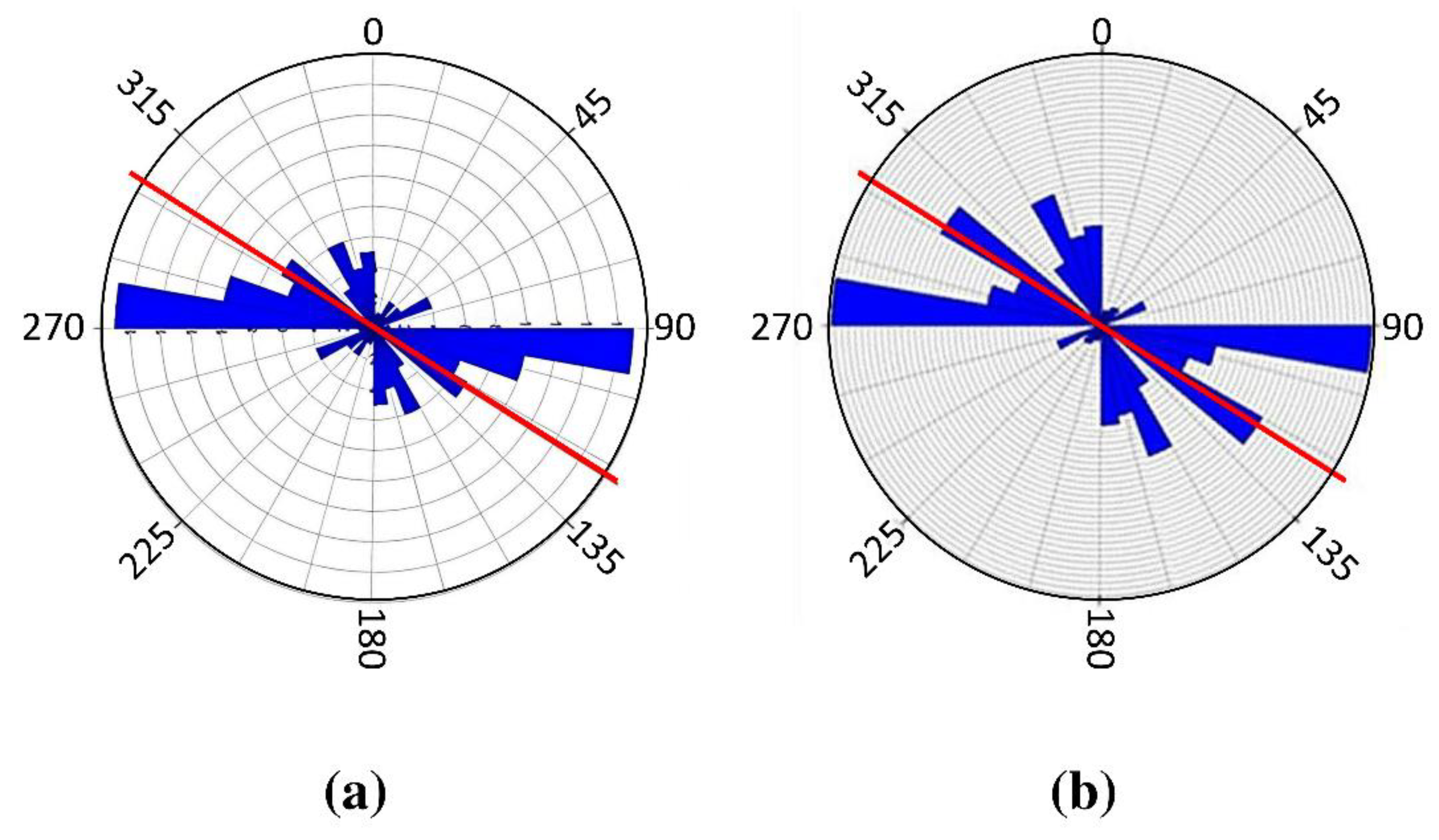
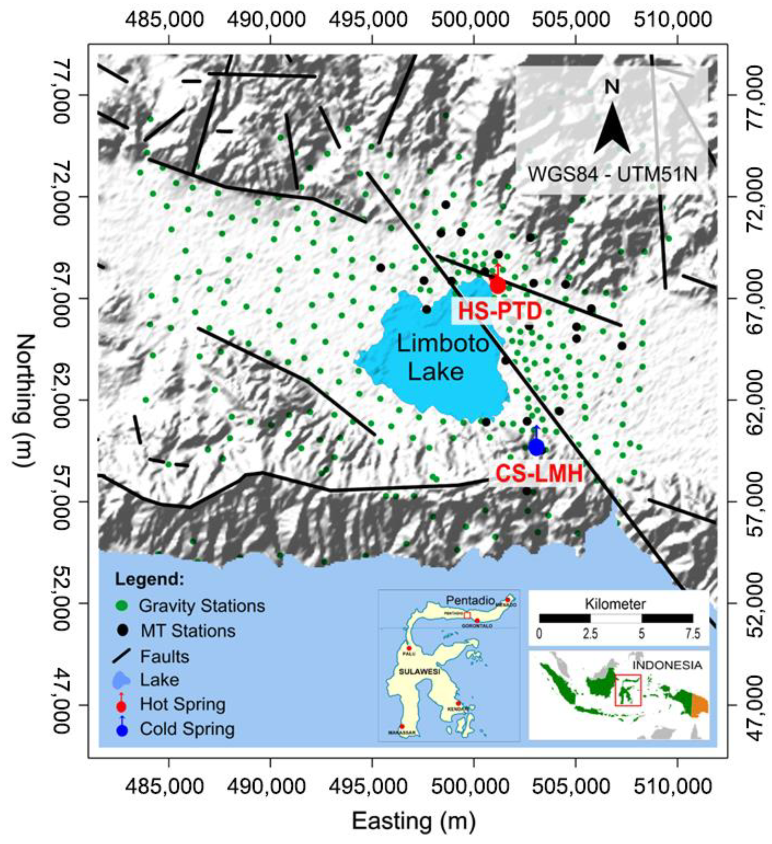
Fault System of Limboto Lake—Pentadio

The faults and fractures mapped in the area are normal faults and lineaments, which are difficult to identify. In general, the fault structures have relatively W–E- and northwest–southeast (NW–SE)-trending orientations, as depicted by the rose diagrams in Figure 2. The frequency of faults and fractures in the study area (Figure 2a) displays a dominant W–E orientation. In contrast, the length of the stretch of faults and fractures (Figure 2b) has a dominant orientation in a relatively W–E and NW–SE direction. The W–E-striking faults are normal-step faults that yield the Gorontalo Depression Zone in the form of an elongated plain morphology, within which Limboto Lake is located.

The graben zone is oriented in the same manner as the regional geological formation that generates the Limboto–Bone Rift depression zone. The faults and their relatively NW–SE-trending associated fractures are interpreted as dextral slip faults that cut the geological structure in the W–E direction. The depression zone affects the volcanism in the area. The fault zone architecture, which is formed in the depression zone, together with its associated rock permeability, characterizes the fluid flow in the area [35]. The faults and their associated fracture systems in the depression zone serve as controls for the subsurface fluid flow system. The appearance of hot springs in the Limboto Lake—Pentadio area, which is in the depression zone, provides evidence of the influence of fractures producing normal faults that carry geothermal fluids to the surface.

3. MT Method

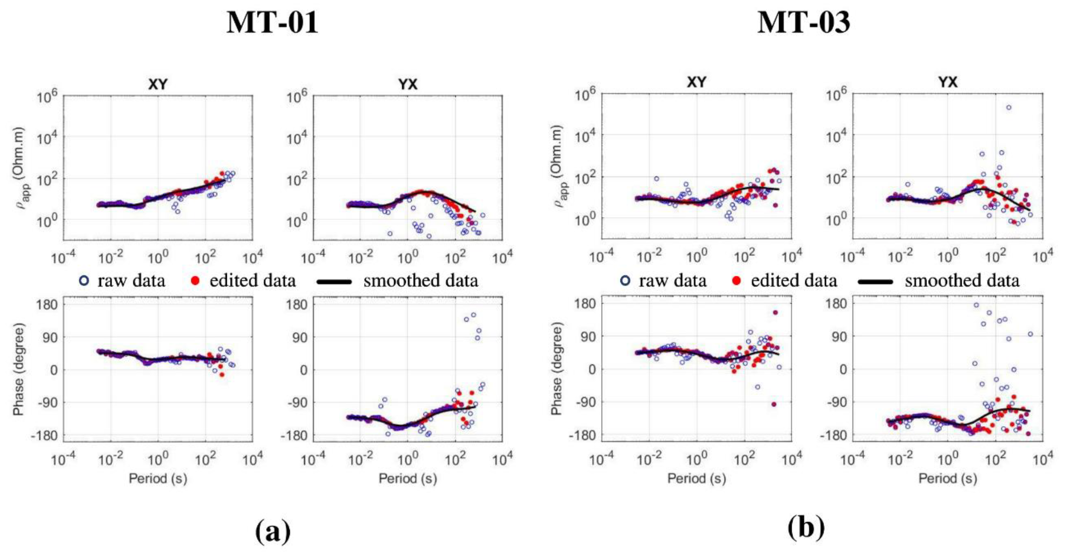
3.1. MT Data Acquisition and Processing

MT is an electromagnetic (EM) method that measures the time-varying natural electric field $E$ and the magnetic field $H$ at the surface to provide information regarding the distribution of resistivity in the subsurface. The ratio of the electric field to the magnetic field is expressed as an impedance tensor $Z$ that correlates to the electrical resistivity $\rho$ [36,37]:

$$E=ZH,$$

(1)

$$Z=\left[\begin{array}{cc}{Z}_{xx}& Z_{xy}\\ Z_{yx}& Z_{yy}\end{array}\right].$$

(2)

The apparent resistivity and phase that represent the measured data can be expressed as follows:

$${\rho }_a=\frac{1}{\omega \mu }{\left|Z\right|}^2,$$

(3)

$$\phi ={\tan }^{-1}\left(\frac{Im\left(Z\right)}{Re\left(Z\right)}\right).$$

(4)

Five EM field components were acquired during the measurements. There were two mutually orthogonal electric field components ($E_x$ and $E_y$) and three mutually orthogonal magnetic field components ($H_x$, $H_y$, and $H_z$). Thirty-two MT stations were distributed throughout the study area, covering 73 km² near Limboto Lake, including the Gorontalo Fault and the surface manifestation area (Figure 3). The spacing between the stations was 1–2 km. The MT data were collected in 2013 using MTU-5A units manufactured by Phoenix Geophysics Ltd., Toronto, ON, Canada [38]. The EM time-series data were recorded for 8–22 h to obtain optimal MT transfer functions that fulfilled the need for adequate penetration and good data quality. The measurement period ranged from 3.125 × 10⁻³ to 104 s. The noise measured in the field was caused by the settlements and activities of residents around Limboto Lake, Pentadio.

The time-series data were converted into frequency domain data by the Fourier-transform process, yielding other types of data that were expressed as apparent resistivities and impedance phases. In general, the data quality was good (up to 1 s). The curves of the apparent resistivity and impedance phase for all measuring stations are shown in Supplementary Material 1. Over longer periods, the data quality decreased because of the lack of data stacking in these range periods. Quality improvement of the measured data was achieved by performing a cross-power selection process. This cross-power selection process was guided by the dispersion relation [39]:

$$\varphi \left(\omega \right)=\frac{\pi }{4}-\frac{\omega }{4}{{\displaystyle \int }}_0^{\infty }log\frac{{\rho }_a\left(x\right)}{{\rho }_0}\frac{dx}{x^2-{\omega }^2}.$$

(5)

Based on the principle of causality, this relationship indicates that neighboring frequencies provide similar transfer functions. This implies that the apparent resistivity at a certain frequency ${\rho }_a$(x) can be estimated from the impedance phase at the next neighboring frequency $\varphi \left(\omega \right)$. The data were then smoothed by cubic spline interpolation. Figure 4 depicts a comparison among the three types of apparent resistivity and phase curves for MT-01 and MT-03. The first is the raw data (denoted by blue circles), the cross-power selected data (denoted by red solid circles), and the final data, which were generated by interpolating the cross-power selected data (denoted by black solid lines). Smaller error bars were observed in the last type of data for longer periods.

Figure 5 depicts the rose diagrams of the regional conductivity strikes calculated from the MT data using the Groom–Bailey decomposition technique for each site at multiple frequencies [40]. The existence of a geological strike can be verified based on this regional conductivity strike and vice versa. The geological strike typically corresponds to one strike direction out of the two possible strike directions that are perpendicular to each other [41,42]. By comparing Figure 2 and Figure 5, the average value of the direction of the conductivity strike in the measurement area was shown to be relatively east–west with an angle of N 113.6° E. The identification of the geological strike direction, with the help of the conductivity strike direction, is useful in modeling the density structure from gravity data and in developing a conceptual model of the geothermal system beneath Limboto Lake—Pentadio.

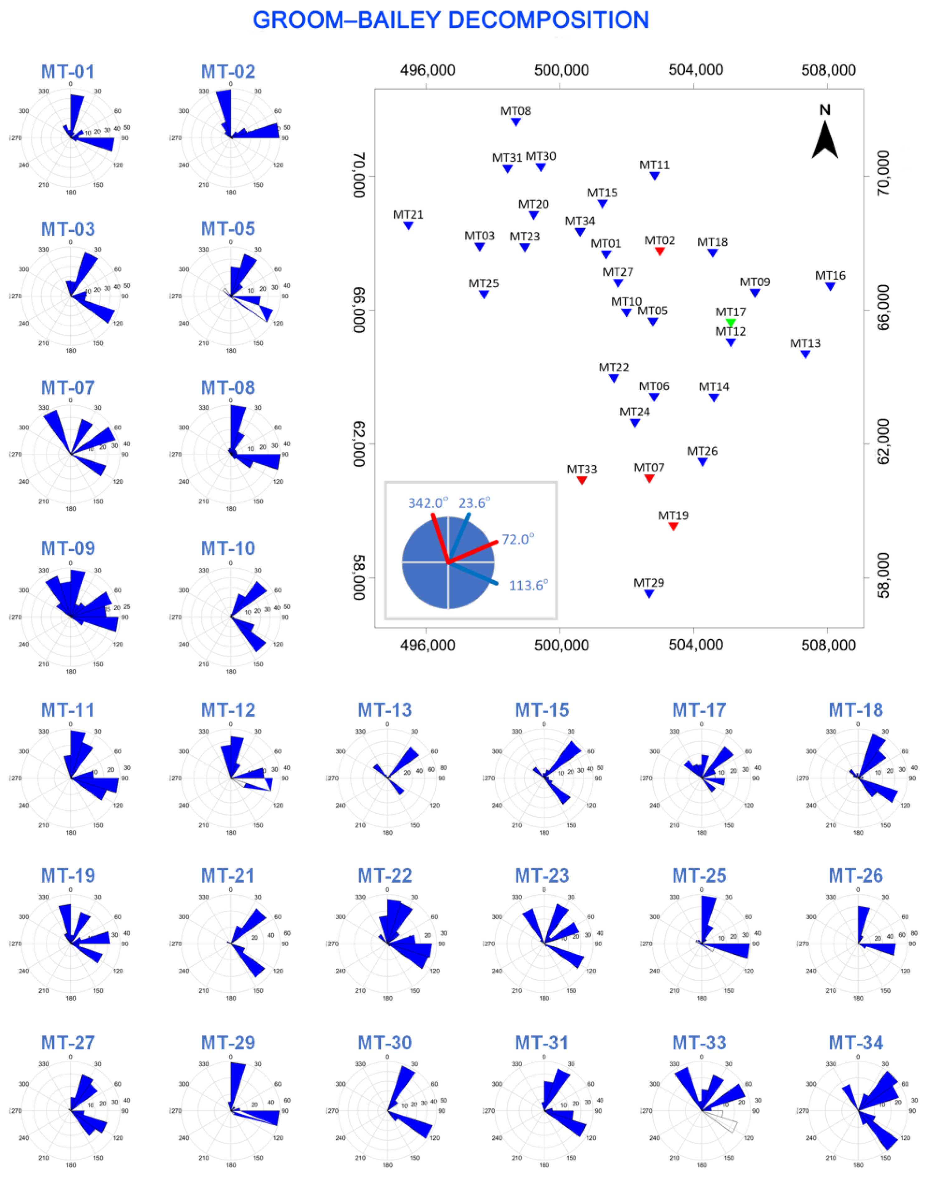
3.2. 3D MT Inversion

The 3D inversion to transform the data into information for a preferred resistivity model was conducted using the WS3DINVMT code [43]. The smoothest models were achieved by finding stationary points of an unconstrained functional $U\left(m,\lambda \right)$:

$$U\left(m,\lambda \right)={\left(m-m_0\right)}^T{C}_m^{-1}\left(m-m_0\right)+{\lambda }^{-1}\left\{{\left(d-F\left[m\right]\right)}^T{C}_d^{-1}\left(d-F\left[m\right]\right)-X^{*2}\right\}.$$

(6)

where $m$ is the resistivity model, $m_0$ is the prior model, $C_m$ is the model covariance matrix, $d$ is the observed data, $F\left[m\right]$ is the model response, $C_d$ is the data covariance matrix, ${\lambda }^{-1}$ is the Lagrange multiplier, and $X^{*}$ is the misfit level.

The 3D MT inversion was performed for 26 MT datasets from 32 MT stations. We excluded six datasets because of their poor quality. In this 3D inversion, four response parameters were used: the real and imaginary parts of the off-diagonal impedances, $Z_{xy}$, and $Z_{yx}$. Several 3D MT inversion studies have used only the off-diagonal impedance tensor for the inversion process because the magnitudes of the diagonal components ($Z_{xx}$ and $Z_{yy}$) were too small and the errors were too large [44,45,46,47]. To reduce the computational loads, the data were resampled to include 10 period values out of 72–80 values from the 3.125 × 10⁻³ to 104 s period range.

The impedance data were inverted using a 3D model comprised of meshes, where the smallest mesh dimension in the horizontal direction was 500 m × 500 m. Outside the coverage area where the MT stations were distributed, the mesh dimensions were increased laterally by a factor of 1.2 to avoid the boundary effects of the modeling domain. The first vertical thickness of the ground was set to 100 m, followed by an increase in thickness in the vertical direction by a factor of 1.2. The total number of meshes in the $x$, $y$, and $z$ directions was 48, 48, and 28, respectively. A homogeneous half-space initial model of 100 Ωm was used in the inversion scheme.

A final 3D resistivity model was obtained after 10 iterations and ~120 h of computing time, with a root mean square (RMS) misfit of 2.685. Figure 6 depicts an example comparison between the observed and calculated data from MT-01 and MT-03 (for all stations provided in Supplementary Material 2. Figure 7 shows a comparison between the observed and calculated data in terms of the apparent resistivity and impedance phase maps, as well as their RMS values (for all periods provided in Supplementary Material 3). The highest and lowest periods involved in the inversion process were 3.125 × 10⁻³ and 50 s, respectively. At 0.003 s, the apparent resistivity had the highest RMS value (1.41) for the $yx$-data components. The lowest RMS value of the apparent resistivity was 0.2 at a period of 0.001 s for the $xy$-data components. In contrast, the impedance phase had the highest RMS value at a period of 50 s with an RMS value of 14.88 for the $xy$-data components. The lowest RMS value of the impedance phase was 8.74 at a period of 2.0408 s for the $yx$-data components. In general, the calculated data maps resembled the observed data maps, apart from the frequency values.

4. Gravity Method

4.1. Gravity Data Acquisition and Reduction

The gravity survey was conducted concurrently with the MT survey using a Lacoste and Romberg G-655 unit. The survey covered an area of 500 km² and 319 gravity stations were distributed (Figure 3). The distance between each measurement point ranged between 250 and 500 m. Most of the measurement stations were concentrated near Limboto Lake and the location of the geothermal surface manifestations. The base station for the gravity survey was located in Limboto Village at X = 498,445.535 and Y = 68,914.608 (UTM coordinates of WGS84, Zone 51) at an elevation of 5653 masl. The gravity value of the base station was first tied to the nearest national gravity value at Jalaluddin Airport, Gorontalo City at X = 483,587 and Y = 70,571, situated at an elevation of 30 masl with a gravity absolute value (Gabs) of 978,093.59 mGal. The Gabs of the base station was found to be 978,100.244346 mGal.

The gravity method measures variations in gravity acceleration on the surface due to variations in the rock density values below the surface. The measured data are affected by the drift effect, tidal effect, latitude, altitude from the surface, and terrain effect. Data reduction must be applied to obtain a complete Bouguer anomaly (CBA). The CBA (in mGal) at a certain position was estimated using the following equation [48]:

$$BA=g-\gamma +\beta h-2\pi G\rho h+\rho T$$

(7)

where $g$ (mGal) is the observed absolute gravity, $\gamma$ (mGal) is the normal gravity value, $\beta h$ (mGal/m) is the free-air correction, and $T$ is the terrain correction per unit average density. $G$ (m³ kg⁻¹ s⁻²), $\rho$ (kg m⁻³), and h (m) are the universal gravitational constant, density, and elevation, respectively. To obtain accurate Bouguer and terrain corrections, a proper estimation of the rock density values is needed. The rock density was determined before the Bouguer correction using the Parasnis method. The Bouguer anomaly is described as a function of density. Density values were estimated by minimizing the sum of the differences between the average Bouguer anomalies from the entire area with respect to the Bouguer anomaly at each observation point [49]. Based on these estimation results, a density correction value of 2.5 g/cm³ was used in gravity data processing. Terrain corrections were calculated using a 50 m digital elevation model (DEM). The corrected data are the CBA used in the gravity analysis.

4.1.1. The Regional Separation: Polynomial Regression

The CBA map contains anomaly superpositions from several sources below the surface. A long-wavelength anomaly (associated with deep objects) is called a regional anomaly. Regional anomalies are important for understanding the large-scale structures beneath the main geographical features, such as mountains, oceanic ridges, and subduction zones. The short-wavelength anomaly (caused by shallow mass objects) is referred to as the residual anomaly. The regional-residual separation of CBA was conducted using a polynomial regression technique. In this method, regional trends are represented by a polynomial equation derived from the regression calculation. The regional anomalies, using second-order polynomial regression, can be written as [50]:

$$\Delta g\left(x,y\right)=\Delta g_0+\Delta g_{\mathrm{x}1}\mathrm{x}+\Delta g_{\mathrm{y}1}\mathrm{y}+\Delta g_2{\mathrm{x}}^2+\Delta g_{\mathrm{y}2}{\mathrm{y}}^2+\Delta g_{x\mathrm{y}}\mathrm{xy}.$$

(8)

The values of all the coefficients in Equation (8) were determined using the least-squares method. The residual anomalies at each station were calculated by subtracting the regional anomalies over the CBA.

4.1.2. Gradient Analysis

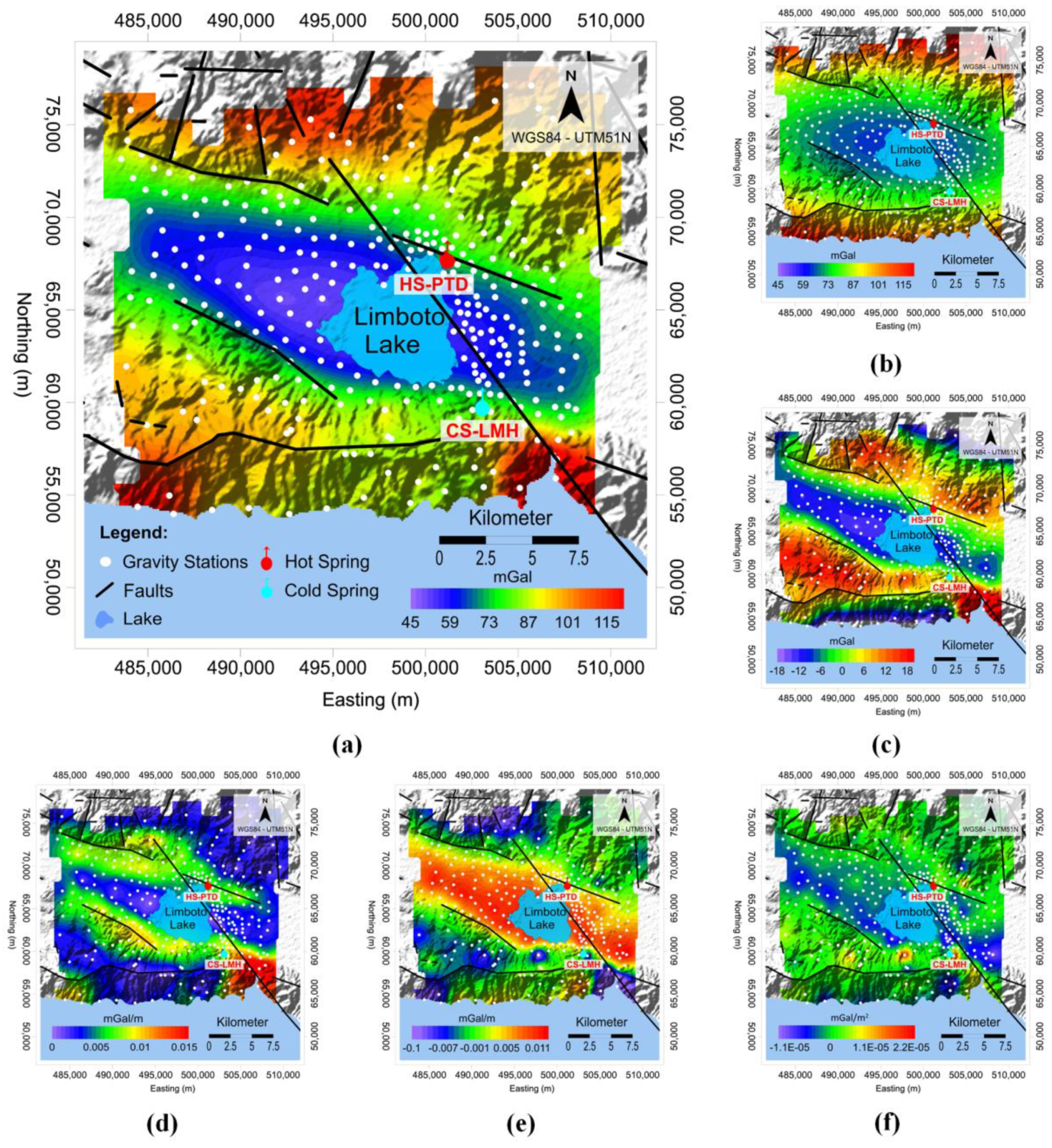
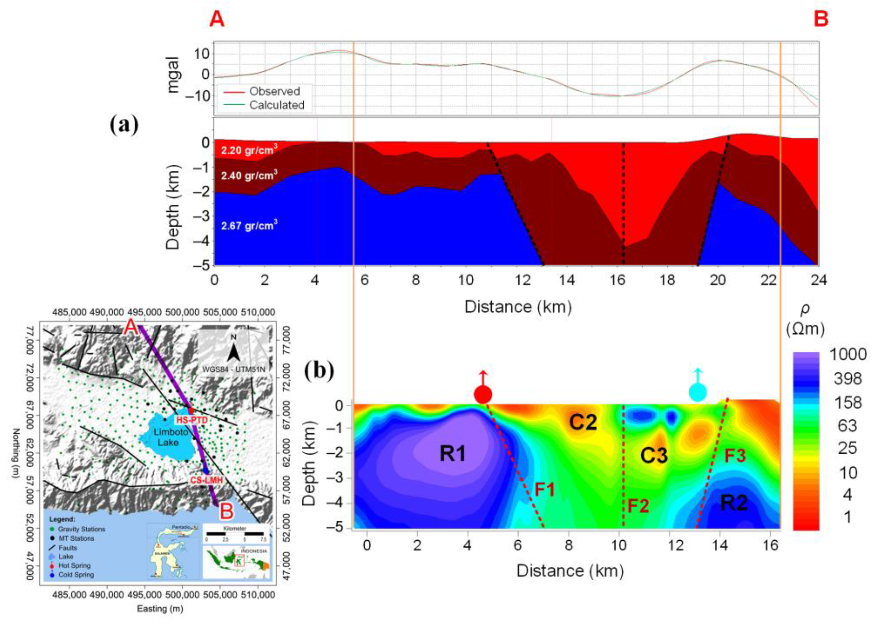
This method is used to determine geometric parameters, such as the boundary location and depth of the source body. Horizontal gradient analyses have been widely used to localize the lateral density contrast from gravity data. This analysis is less susceptible to artifact interference in the data because it only requires the calculation of the two first-order horizontal derivatives. This method is useful for enhancing both the shallow and deep sources [51]. The amplitude of the horizontal gradient is expressed as:

$$H{G}_g=\sqrt{{\left(\frac{\partial g}{\partial x}\right)}^2+{\left(\frac{\partial g}{\partial y}\right)}^2},$$

(9)

where $\left(\frac{\partial g}{\partial x}\right)$ and $\left(\frac{\partial g}{\partial y}\right)$ are the horizontal derivatives of the gravitational field in the $x$ and $y$ directions, respectively.

A vertical gradient analysis was used to localize the vertical density contrast boundary from the gravity data. The amplitude of the vertical gradient is expressed as:

$$V{G}_g=\left(\frac{\partial g}{\partial z}\right).$$

(10)

We used a second-derivative analysis (SVD) to distinguish the local geological features from the regional ones. An SVD image often provides a clearer and improved description of the anomaly, especially on its important exploration properties, compared with the CBA [52]. Moreover, this analysis is advantageous. It is highly sensitive to small errors in gravity measurements. An SVD analysis covers the calculation of $\frac{{\partial }^{2}g}{\partial x^2}$ and $\frac{{\partial }^{2}g}{\partial y^2}$ from the gravity field. From the Laplace equation, it has been proven that the sum of the horizontal gradient produces $\frac{{\partial }^{2}g}{\partial z^2}$ with the opposite sign.

5. Results

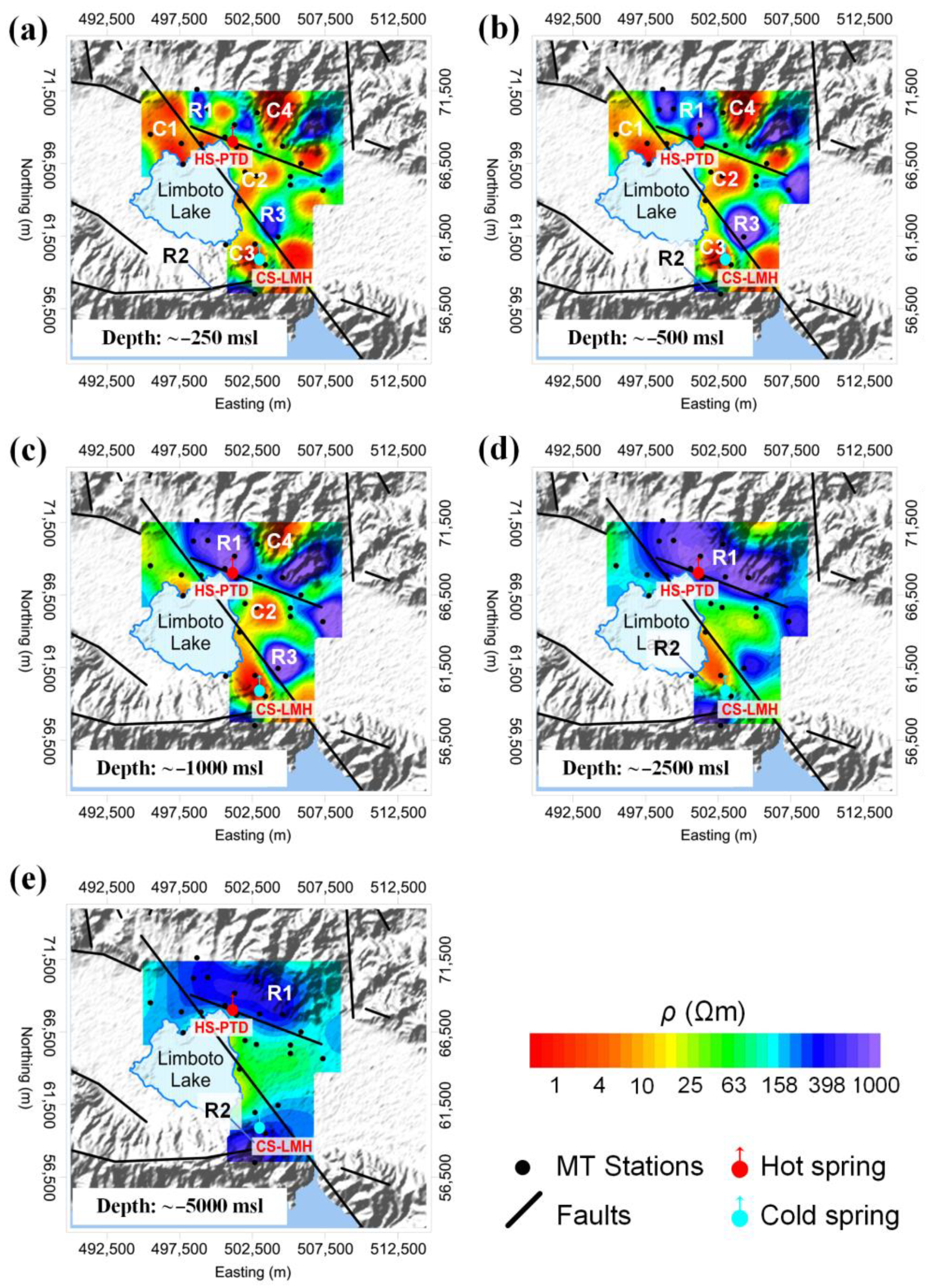
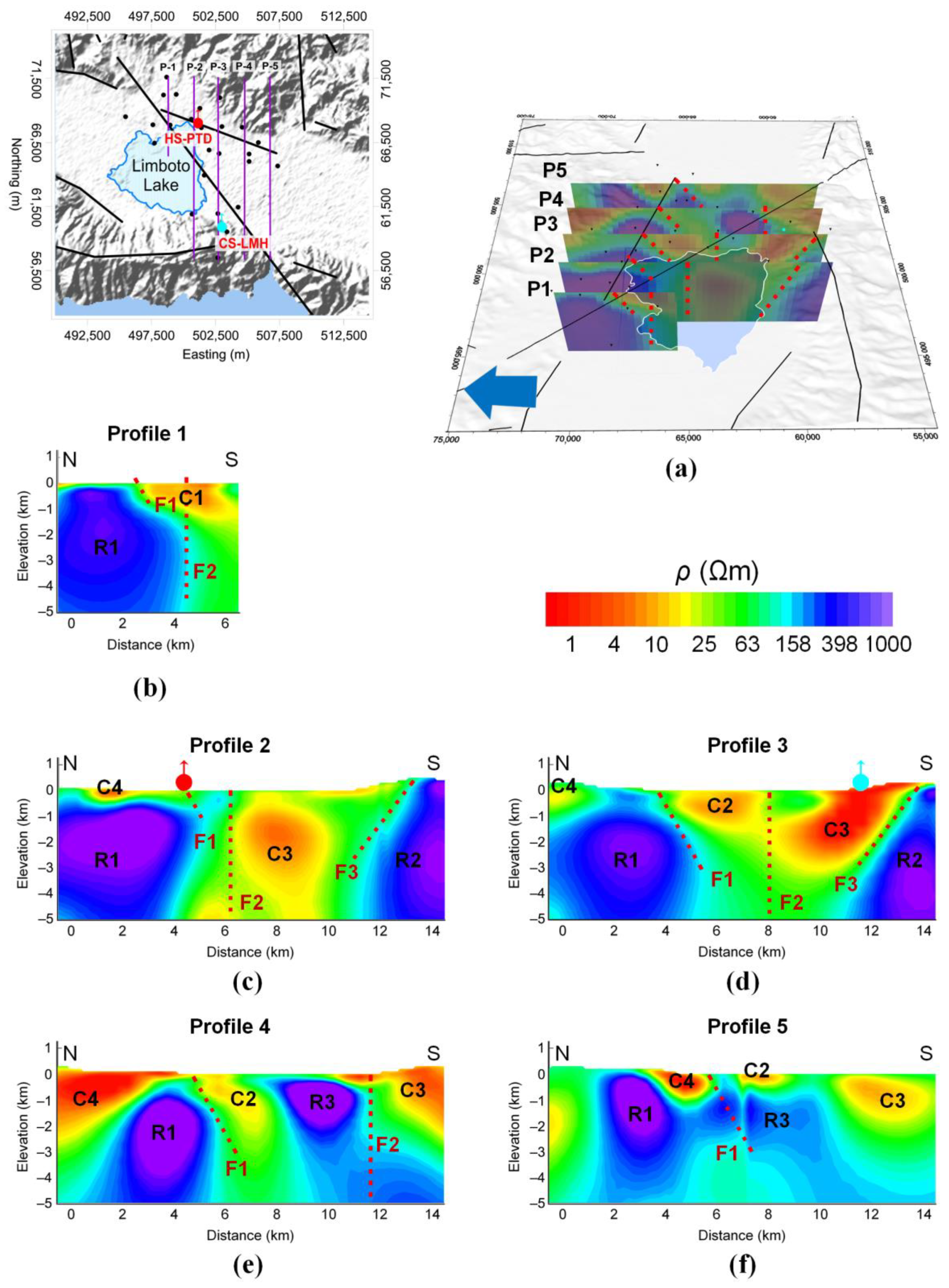
5.1. 3D Resistivity Structure of Limboto Lake, Pentadio

The preferred 3D resistivity model of Limboto Lake, Pentadio is presented in Figure 8 and Figure 9. Figure 8 shows the horizontal cross-sections at several depths from ~−250 to −5000 msl. The main resistivity anomalies were divided into conductive (C1, C2, C3, and C4) and resistive (R1, R2, and R3) zones for convenience during the analysis. The resistivity values were heterogeneous at shallow depths (~−250 msl). There was a conductive zone (~1–15 Ωm) surrounded by a moderate resistivity structure (~20–90 Ωm). In addition, there was a resistive zone (~100–1000 Ωm) from north to east and southeast. The conductive zones (C1, C2, and C3) may be attributed to lake deposits serving as fillers in the Gorontalo graben zone. Conductive zone C4 in the northeastern part was likely a weathered intrusive rock that has become soil. The geothermal manifestations were located in the fault or fracture zone, which was also in conductive zone C2. At a depth of ~−500 msl, the resistivity exhibited a fairly clear structural pattern. This pattern showed a clear resistivity structural boundary between the conductive and resistive zones. Resistive zone R1 in the north and northeast extended relatively deep (~−5000 msl). This feature may be related to the presence of andesitic lava in the north and intrusive rocks in the northeast, which extend to the east. The appearance of resistive zone R3 in the southeastern part of the study area was associated with granitic rocks as intrusive rocks near the surface. A clear boundary between the conductive and resistive zones showed a pattern of faults and fractures trending NW–SE and W–E, forming the Gorontalo graben zone.

Figure 9a depicts the five profiles of the preferred model in a 3D view extracted from the 3D resistivity model. The red dashed lines (F1, F2, and F3) represent faults based on the resistivity profile. In the middle of the study area, an elongated conductive feature was observed, trending nearly NW–SE. This elongated conductor was constrained by the resistive zone in the northern area, which widens to the east. These cross-sections can also be used to image the tectonic features throughout the study area. This feature gives an overview of the graben structure and indicates the presence of the Gorontalo Fault (F2), marked by a resistivity discontinuity. The existence of a fault characterized by a resistivity discontinuity that reflects several possibilities, namely differences in rocks or textures, or differences in the water content of fault zones embedded in rock formations, has also been stated by several authors (e.g., [42,53,54,55,56,57]).

Figure 9b shows an N–S resistivity section (Profile-1) located in the northern part of the Limboto Lake—Pentadio area. Profile-1 shows that in the north area, a very thick resistor, R1, existed extending from the ~−250–−5000 m depth and may correspond to andesitic lava as an old volcano product. This section suggested the presence of a resistivity discontinuity, which may be attributed to faults F1 and F2. A conductor labeled C1 existed near the surface and was connected to a moderate resistivity body in the Gorontalo graben zone.

Profile-2 in Figure 9c shows a resistivity discontinuity between conductive zone C4 and resistive zone R1, which may reflect the presence of a fault. This interpretation was supported by the presence of a hot spring complex at the superficial tip of the interpreted fault. According to field data, there were five nearby hot springs: MAP-PTD-01, MAP-PTD-02, MAP-PTD-03, MAP-PTD-04, and MAP-PTD-05, with water temperatures ranging from 74.8 to 78.5 °C. It is common in geothermal systems to find hot springs in the vicinity of faults [58,59]. A large conductive zone, C3, appeared in the center of the study area and was confined by resistor R2 in the southern area. C3 corresponded to alluvial deposits flanking R1 and R2. R1 corresponded to the lava intrusion in the northern and southern sections, whereas R2 was attributed to the presence of limestone and intrusive rocks. This reflects the existence of grabens filled with alluvium deposits. A resistivity contrast was observed in the middle of the sections, which agrees with the presence of the NW–SE diagonal fault F2 traversing the area.

Profile-3 (Figure 9d) has a feature that is almost identical to one in Profile-2. In general, there was a conductive zone in the center of the study area, confined by two resistive zones (R1 and R2). Profile-4 (Figure 9e) shows the distribution of resistors R1 and R3, which were interrupted by conductor C2. Resistor R1 emerged on the surface and was overlain by conductor C4. Profile-5 (Figure 9f) indicates that the conductive zone became narrower and shallower to the east. All the previously mentioned sections support the interpretation that a W–E-directed graben zone traverses the area. Together with the NW–SE Gorontalo Fault, the above graben zone may have controlled the characteristics of a potential geothermal system in the study area, as indicated by its geothermal surface manifestations.

5.2. Gravity Results

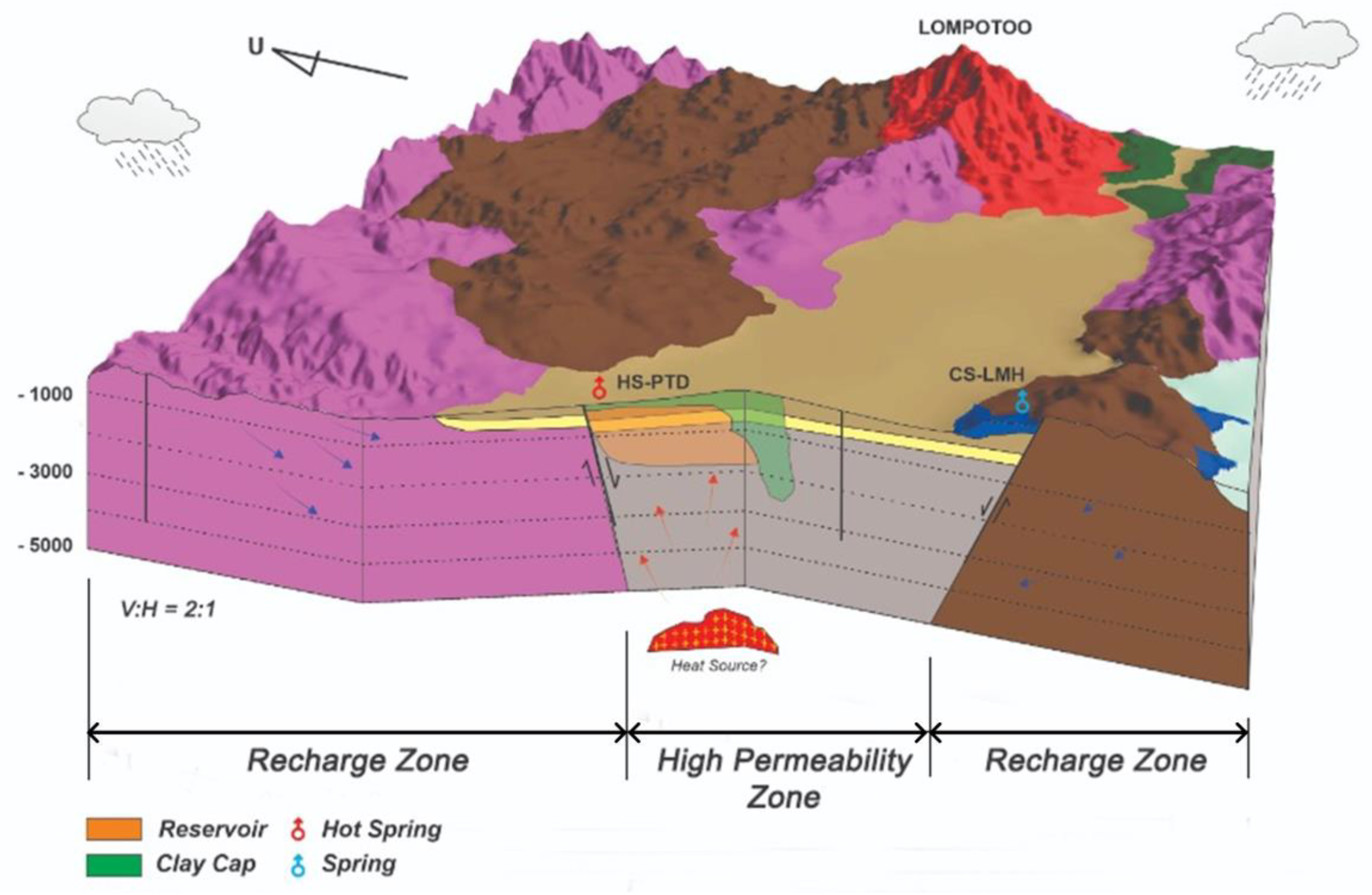
The CBA map depicted in Figure 10a shows values ranging from 47 to 119 mGal. There were high anomaly values in the north and south, which flanked low anomaly values near Limboto Lake. The distribution of the gravity anomaly showed a W–E striking lineament, which indicated the presence of a depression zone. The high anomaly values in the northern and southern sections correlated with the presence of intrusive rocks and andesitic lava, which are volcanic products of old volcanoes. The moderate anomaly values were associated with limestone and sandstone, in accordance with geological studies. The low anomaly values in the center of the study area were associated with low-density materials, reflecting alluvial deposits. These anomalous contrasts indicated that a depression zone was formed by tectonic activity.

The separation of CBA anomalies was performed to obtain information related to local geothermal targets from their regional structures. The separation was performed by subtracting the CBA from a polynomial surface, which represented regional surface tendencies. The second-order polynomial was the most suitable regional anomaly representation. This regional anomaly map (Figure 10b) showed an anomaly distribution that extended W–E, and its values increased to the north and south. These features clarified the symmetrical pattern of the anomaly. The high anomaly zones in the northern and southern sections were associated with the presence of andesitic lava and more massive intrusions compared with the central section, which was filled with limestone and alluvial deposits.

The residual anomaly map (Figure 10c) showed anomalous contrasts that emphasized the presence of recognized lineaments from the CBA. The high anomaly zones were associated with the presence of intrusive rocks, and andesitic lava flanking the limestone and lake sediment in the center of the study area appeared more clearly defined. The locations of geothermal manifestations in the Limboto Lake—Pentadio area were in a transition zone between low and high anomaly zones, which may be attributed to the presence of faults or fracture structures that control the geothermal system in the shallow areas.

Figure 10d depicts the horizontal gradient map that indicated the presence of high anomaly values in the southeastern section of the study area, which may be attributed to the existence of intrusive rocks. The NW–SE-trending lineaments flanking the alluvial zone were clearly visible. These lineaments describe a fairly high-to-medium lateral variation that controls the geothermal system, as evidenced by the presence of a geothermal surface manifestation complex. This manifestation complex was located in the transition between the high and low zones, reflecting horizontal discontinuities or faults.

The vertical gradient analysis sharpened the anomaly over more regional structures and reduced the anomaly complexity, enabling the visualization of the causative body. The vertical gradient amplitude of the study area is illustrated in Figure 10e. The high gradient values around Limboto Lake indicated the presence of high-density rock close to the filling material of the depression zone. The geothermal manifestation zone was observed in the transition area between the high and medium gradients, as is common in geothermal areas [51]. This transition area was associated with faults that have the potential to act as geothermal fluid pathways to the surface.

The SVD map for Limboto Lake, Pentadio is shown in Figure 10f. SVD anomalies are related to shallow and local features, which are equivalent to the results of high-frequency filtering. The highly valued features in the southern and northern sections of the study area bounding the low-valued features in the central section, especially the W–E-trending lines demarcating the limestone and alluvial zones, were extremely clear. The geothermal surface manifestation complex was situated in the transitional zone between the zero and high values, which reflects the presence of faults or fractures.

6. Discussion

The results of our geophysical studies are discussed here to obtain a clear picture of the resistivity structure and existence of geothermal potential in the study area. The 3D resistivity model showed that the conductive structure strikes W–E, which indicates the presence of the Gorontalo graben zone. This is consistent with the low CBA values that extend nearly W–E. These two features frequently occur in the fault zones of geothermal systems [60]. The contrast between the conductive and resistive zones, based on the 3D resistivity model, also characterized the presence of faults and fractures that are dominant in the NW–SE direction. The boundaries of these faults and fractures were clearly visible on the CBA and residual anomaly maps, which showed contrasts between low and high anomalies.

The history of volcanism in the Limboto Lake—Pentadio area is related to the regional tectonic system in the Gorontalo area through rifting and uplift after the Sula Platform collision and the appearance of the North Sulawesi Trench subduction pathway during the Late Miocene to the Quaternary periods. The appearance of the Pilomba and Lompotoo volcanoes in the Gorontalo graben zone was interpreted as the youngest Pleistocene volcanism controlled by the fracture system in the depression zone. The two volcanoes formed through the dyke system in the Gorontalo Depression Zone. The increasing values of the vertical anomaly gradient indicated the presence of high-density rock at a depth near the graben zone fill material, as shown in Figure 10e. This could be related to the situation in which a high-density body representing an intrusive rock or dyke system appears beneath the graben zone. Furthermore, the SVD analysis of gravity showed localized high-value features in the southern and northern sections, indicating the boundaries of the intrusive body or dyke system (Figure 10f). This condition agrees with the 3D MT inversion results, which yielded high resistivity contrasts at the boundaries of the Gorontalo graben zone, where geothermal surface manifestations were located. The high resistivity contrasts located at the boundaries of the Gorontalo graben zone were related to the elongated heat source, according to the geological analysis.

The reservoir of the geothermal system beneath the study area belongs to the Gorontalo graben system. This reservoir is situated in a fracture zone that resulted from the rifting and uplift described in the previous section. Reservoir and clay cap zones can be seen in the resistivity model profile shown in Figure 9 (P3, P4, and P5). Conductive body C2, found near the surface, could be associated with the clay cap, whereas the reservoir was indicated by moderate resistivity values ranging from 60 to 100 Ωm underlain by the conductive body.

Two-dimensional (2D) gravity forward modeling was performed by incorporating the MT and geological results to reduce the possible ambiguity in the resulting 2D density model. We used the CBA as the observed data for the forward modeling scheme. The subsurface density models were developed such that the observed data were fitted using the calculated data generated by certain models. Figure 9a depicts the 2D density model. The model consisted of three layers with different density values. These three density values were determined according to [61]. The associated rock units were obtained from the geological map shown in Figure 1. The lowermost layer of density was bedrock, constituted by granitic rock with a density of 2.67 g/cm³. The overlying bedrock was a low-density rock with a density of 2.4 g/cm³ and was associated with andesitic lava. The topmost layer, with a density of 2.2 g/cm³, corresponded to alluvium deposits filling the graben zone. The density profile confirmed the presence of graben structures in the study area.

There was conformity between the cross-sectional model from the gravity results and the resistivity model from the MT inversion, as shown in Figure 11. The resistivity model on profiles A–B can provide a clear picture of the graben structure, which was marked by the contrasting resistivity values. In addition, near the surface, conductive layer C2 could be interpreted as a clay cap, which is an alluvium deposit that has been altered, giving it a more conductive value. Below this layer, the presence of a reservoir zone was observed with moderate resistivity values.

The integration results based on gravity and the MT method were used to reconstruct a conceptual model of the geothermal system in the Limboto Lake—Pentadio area (Figure 12). The geothermal system included several parameters: reservoir zone heat sources, cover layers, hot fluid sources, and the hydrological cycle [18,19,20]. The model illustrated that the recharge area for the geothermal system in the study area was the upper slope of the Gorontalo graben zone, as an infiltration zone of rainwater that enters the ground into meteoric water and is heated by the dike system below the graben zone until it is trapped in the geothermal reservoir system. The geothermal fluid flow cycle, which is limited to the Gorontalo graben zone, undergoes forced convection until it finally arrives on the Earth’s surface to form hot springs. Before reaching the surface, the fluid condenses at a depth to form steam-heated water, an indication of meteoric water heated by steam in the system. The appearance of the Pentadio hot water is an up-flow zone representing the geothermal reservoir zone below it and the geothermal prospect area on the surface. The Limboto Lake—Pentadio geothermal reservoir was identified based on a resistive layer at 60–80 Ωm recorded from a depth of −750 msl, with a thickness varying between −750 msl and −1250 msl in the andesitic lava rock group. The lateral dimensions of the geothermal system reservoir in the study area formed a separate lenticular pattern (lens) in several segments. This condition was interpreted as the influence of the subsurface geological structural system on the Gorontalo graben zone.

7. Conclusions

The Gorontalo graben zone is a weak zone with open fractures and high permeability. Water can easily penetrate rock owing to its high permeability, causing it to become a water catchment (discharge) area. Furthermore, the Gorontalo graben zone controls and confines subsurface fluid circulation, ensuring a continuous supply of meteoric water into the geothermal system and thus supporting the Pentadio geothermal energy conservation system. The appearance of hot springs in the graben zone shows that the geological structure controls the geothermal system and serves as a conduit for geothermal fluids to reach the surface. Meteoric water infiltration is circulated by convective currents and reappears on the graben zone surface. These features agree with the results of [62,63] when considering the relationship between the presence of a conductive zone and a fault system, as well as geothermal fluids.

The 3D resistivity model of the Limboto Lake—Pentadio area was obtained by inverting MT data from 26 stations. The model confirmed the presence of fault and graben systems as the controlling factors of the regional geothermal system. The graben system is filled with conductive bodies (~1–15 Ωm) corresponding to alluvium deposits, which are flanked by resistive bodies (~100–1000 Ωm) representing andesitic and granitic lavas. The emergence of a hot spring complex confirms the existence of a fault system in the Limboto Lake—Pentadio area as a conduit for geothermal fluids to reach the surface. The fault and graben systems were confirmed from the present geological study and the 2D density model.

References

1. Massinai, M.A.; Harimei, B.; Agustiawati, A.; Massinai, M.F.I. Seismicity Analysis Sulawesi North Arm Based on B-Values. J. Phys. Conf. Ser. 2019, 1341, 082032. [Google Scholar] [CrossRef] [Green Version]
2. Cummins, P.R.; Meilano, I. Geohazards in Indonesia: Earth Science for Disaster Risk Reduction-Introduction. Geol. Soc. Spec. Publ. 2017, 441, 1–7. [Google Scholar] [CrossRef]
3. Putra, S.S.; Hassan, C.; Djudi; Suryatmojo, H. Reservoir Saboworks Solutions in Limboto Lake Sedimentations, Northern Sulawesi, Indonesia. Procedia Environ. Sci. 2013, 17, 230–239. [Google Scholar] [CrossRef] [Green Version]
4. Andri Kurniawan, I.; Sugawara, H.; Sakakibara, M.; Arifin Indriati, Y.; Suly Eraku, S. The Potential of Gorontalo Province as Global Geopark. IOP Conf. Ser. Earth Environ. Sci. 2020, 536, 012004. [Google Scholar] [CrossRef]
5. Manyoe, I.N.; Arifin, Y.I.; Napu, S.S.S.; Suma, M.D. Assessment of the Values of Science, Education, Tourism and the Risk Degradation of Pentadio Geothermal Areas to Developing Geotourism in the Limboto Lake Plain, Gorontalo. J. Phys. Conf. Ser. 2021, 1968, 012047. [Google Scholar] [CrossRef]
6. Heise, W.; Caldwell, T.G.; Bibby, H.M.; Bennie, S.L. Three-Dimensional Electrical Resistivity Image of Magma beneath an Active Continental Rift, Taupo Volcanic Zone, New Zealand. Geophys. Res. Lett. 2010, 37, 2–6. [Google Scholar] [CrossRef]
7. Aizawa, K.; Koyama, T.; Hase, H.; Uyeshima, M.; Kanda, W.; Utsugi, M.; Yoshimura, R.; Yamaya, Y.; Hashimoto, T.; Yamazaki, K.; et al. Three-Dimensional Resistivity Structure and Magma Plumbing System of the Kirishima Volcanoes as Inferred from Broadband Magnetotelluric Data. J. Geophys. Res. Solid Earth 2014, 119, 198–215. [Google Scholar] [CrossRef]
8. Ogawa, Y.; Ichiki, M.; Kanda, W.; Mishina, M.; Asamori, K. Three-Dimensional Magnetotelluric Imaging of Crustal Fluids and Seismicity around Naruko Volcano, NE Japan. Earth Planets Space 2014, 66, 158. [Google Scholar] [CrossRef] [Green Version]
9. Bertrand, E.A.; Caldwell, T.G.; Bannister, S.; Soengkono, S.; Bennie, S.L.; Hill, G.J.; Heise, W. Using Array MT Data to Image the Crustal Resistivity Structure of the Southeastern Taupo Volcanic Zone, New Zealand. J. Volcanol. Geotherm. Res. 2015, 305, 63–75. [Google Scholar] [CrossRef]
10. Chouteau, M.; Zhang, P.; Dion, D.J.; Giroux, B.; Morin, R.; Krivochieva, S. Delineating Mineralization and Imaging the Regional Structure with Magnetotellurics in the Region of Chibougamau (Canada). Geophysics 1997, 62, 730–748. [Google Scholar] [CrossRef]
11. Aizawa, K.; Ogawa, Y.; Ishido, T. Groundwater Flow and Hydrothermal Systems within Volcanic Edifices: Delineation by Electric Self-Potential and Magnetotellurics. J. Geophys. Res. Solid Earth 2009, 114, B01208. [Google Scholar] [CrossRef]
12. Zhang, L.; Unsworth, M.; Jin, S.; Wei, W.; Ye, G.; Jones, A.G.; Jing, J.; Dong, H.; Xie, C.; Le Pape, F.; et al. Structure of the Central Altyn Tagh Fault Revealed by Magnetotelluric Data: New Insights into the Structure of the Northern Margin of the India-Asia Collision. Earth Planet. Sci. Lett. 2015, 415, 67–79. [Google Scholar] [CrossRef]
13. Lindsey, N.J.; Newman, G.A. Improved Workflow for 3D Inverse Modeling of Magnetotelluric Data: Examples from Five Geothermal Systems. Geothermics 2015, 53, 527–532. [Google Scholar] [CrossRef] [Green Version]
14. Rosenkjaer, G.K.; Gasperikova, E.; Newman, G.A.; Arnason, K.; Lindsey, N.J. Comparison of 3D MT Inversions for Geothermal Exploration: Case Studies for Krafla and Hengill Geothermal Systems in Iceland. Geothermics 2015, 57, 258–274. [Google Scholar] [CrossRef] [Green Version]
15. Bertrand, E.A.; Unsworth, M.J.; Chiang, C.W.; Chen, C.S.; Chen, C.C.; Wu, F.T.; Türkoǧlu, E.; Hsu, H.L.; Hill, G.J. Magnetotelluric Imaging beneath the Taiwan Orogen: An Arc-Continent Collision. J. Geophys. Res. Solid Earth 2012, 117, B01402. [Google Scholar] [CrossRef]
16. Boonchaisuk, S.; Siripunvaraporn, W.; Ogawa, Y. Evidence for Middle Triassic to Miocene Dual Subduction Zones beneath the Shan-Thai Terrane, Western Thailand from Magnetotelluric Data. Gondwana Res. 2013, 23, 1607–1616. [Google Scholar] [CrossRef]
17. Khoza, T.D.; Jones, A.G.; Muller, M.R.; Evans, R.L.; Miensopust, M.P.; Webb, S.J. Lithospheric Structure of an Archean Craton and Adjacent Mobile Belt Revealed from 2-D and 3-D Inversion of Magnetotelluric Data: Example from Southern Congo Craton in Northern Namibia. J. Geophys. Res. Solid Earth 2013, 118, 4378–4397. [Google Scholar] [CrossRef] [Green Version]
18. Abdallah, S.; Utsugi, M.; Aizawa, K.; Uyeshima, M.; Kanda, W.; Koyama, T.; Shiotani, T. Three-Dimensional Electrical Resistivity Structure of the Kuju Volcanic Group, Central Kyushu, Japan Revealed by Magnetotelluric Survey Data. J. Volcanol. Geotherm. Res. 2020, 400, 106898. [Google Scholar] [CrossRef]
19. Cumming, W. Geothermal Resource Conceptual Models Using Surface Exploration Data. In Proceedings of the Twenty-First Workshop on Geothermal Reservoir Engineering, Standfor University, Standford, CA, USA, 9–11 February 2009. SGP–TR–187. [Google Scholar]
20. Pellerin, L.; Johnston, J.M.; Hohmann, G.W. A Numerical Evaluation of Electromagnetic Methods in Geothermal Exploration. Geophysics 1996, 61, 121–130. [Google Scholar] [CrossRef]
21. Roden, J.; Abdelsalam, M.G.; Atekwana, E.; El-Qady, G.; Tarabees, E.A. Structural Influence on the Evolution of the Pre-Eonile Drainage System of Southern Egypt: Insights from Magnetotelluric and Gravity Data. J. Afr. Earth Sci. 2011, 61, 358–368. [Google Scholar] [CrossRef]
22. Kanda, I.; Fujimitsu, Y.; Nishijima, J. Geological Structures Controlling the Placement and Geometry of Heat Sources within the Menengai Geothermal Field, Kenya as Evidenced by Gravity Study. Geothermics 2019, 79, 67–81. [Google Scholar] [CrossRef]
23. Maithya, J.; Fujimitsu, Y.; Nishijima, J. Analysis of Gravity Data to Delineate Structural Features Controlling the Eburru Geothermal System in Kenya. Geothermics 2020, 85, 101795. [Google Scholar] [CrossRef]
24. Mulugeta, B.D.; Fujimitsu, Y.; Nishijima, J.; Saibi, H. Interpretation of Gravity Data to Delineate the Subsurface Structures and Reservoir Geometry of the Aluto–Langano Geothermal Field, Ethiopia. Geothermics 2021, 94, 102093. [Google Scholar] [CrossRef]
25. Hamilton, W. Tectonics of the Indonesian Region. Bull. Geol. Soc. Malays. 1973, 6, 3–10. [Google Scholar] [CrossRef]
26. Helmers, H. Sulawesi Blueschists and Subduction Along The Sunda Continent, An Alternative View. In Proceedings of the Silver Jubilee Symposium on the Dynamics of Subduction and Its Products, Yogyakarta, Indonesia, 17–19 September 1991; pp. 220–223. [Google Scholar]
27. Simandjuntak, T.O.; Mubroto, M. Neogene Tethyan Type Convergence in Eastern Sulawesi. In Proceedings of the Silver Jubilee Symposium on the Dynamics of Subduction and Its Products, Yogyakarta, Indonesia, 17–19 September 1991; pp. 274–277. [Google Scholar]
28. Sukamto, R. Peta Geologi Tinjau Daerah Palu Sulawesi Tengah Reconnaissance Geologic Map of Palu Area Central Sulawesi; Geological Survey of Indonesia: Bandung, Indonesia, 1973.
29. Kavalieris, I.; van Leeuwen, T.M.; Wilson, M. Geological Setting and Styles of Mineralization, North Arm of Sulawesi, Indonesia. J. Southeast Asian Earth Sci. 1992, 7, 113–129. [Google Scholar] [CrossRef]
30. Bachri, S. Structural Pattern and Stress System Evolution During Neogene-Pleistocene Times in the Central Part of the North Arm of Sulawesi. J. Geol. Dan Sumberd. Miner. 2011, 21, 127–135. [Google Scholar]
31. Sompotan, A.F. Struktur Geologi Sulawesi; Perpustakaan Sains Kebumian Institut Teknologi: Bandung, Indonesia, 2012. [Google Scholar]
32. Apandi, T.; Bachri, S. Geological Map of The Kotamubagu Sheet, Sulawesi. Pus. Penelit. dan Pengemb. Geol. 1997. [Google Scholar]
33. Lowder, G.G.; Dow, J.A.S. Geology and Exploration of Porphyry Copper Deposits Indonesia. Econ. Geol. 1978, 73, 628–644. [Google Scholar] [CrossRef]
34. Perelló, J.A. Geology, Porphyry CuAu, and Epithermal CuAuAg Mineralization of the Tombulilato District, North Sulawesi, Indonesia. J. Geochem. Explor. 1994, 50, 221–256. [Google Scholar] [CrossRef]
35. Caine, J.S.; Evans, J.P.; Forster, C.B. Fault Zone Architecture and Permeability Structure. Geology 1996, 24, 1025–1028. [Google Scholar] [CrossRef]
36. Cagniard, L. Basic Theory of the Magneto-Telluric Method of Geophysical Prospecting. Geophysics 1953, 18, 605–635. [Google Scholar] [CrossRef]
37. Tikhonov, A. On Determining Electrical Characteristics of the Deep Layers of the Earth’s Crust. Doklady 1950, 73, 295–297. [Google Scholar]
38. Phoenix Geophysics. V5 System 2000 MTU/MTU-A User Guide Version 2.0 D; Phoenix Geophysics: Scarborough, ON, Canada, 2010. [Google Scholar]
39. Weidelt, P. The Inverse Problem of Geomagnetic Induction. J. Geophys. 1972, 38, 257–289. [Google Scholar] [CrossRef]
40. Groom, R.W.; Bailey, R.C. Decomposition of Magnetotelluric Impedance Tensors in the Presence of Local Three-Dimensional Galvanic Distortion. J. Geophys. Res. 1989, 94, 1913–1925. [Google Scholar] [CrossRef] [Green Version]
41. Platz, A.; Weckmann, U.; Pek, J.; Kováčiková, S.; Klanica, R.; Mair, J.; Aleid, B. 3D Imaging of the Subsurface Electrical Resistivity Structure in West Bohemia/Upper Palatinate Covering Mofettes and Quaternary Volcanic Structures by Using Magnetotellurics. Tectonophysics 2022, 833, 229353. [Google Scholar] [CrossRef]
42. Triahadini, A.; Aizawa, K.; Teguri, Y.; Koyama, T.; Tsukamoto, K.; Muramatsu, D.; Chiba, K.; Uyeshima, M. Magnetotelluric Transect of Unzen Graben, Japan: Conductors Associated with Normal Faults. Earth Planets Space 2019, 71, 28. [Google Scholar] [CrossRef]
43. Siripunvaraporn, W.; Egbert, G. WSINV3DMT: Vertical Magnetic Field Transfer Function Inversion and Parallel Implementation. Phys. Earth Planet. Inter. 2009, 173, 317–329. [Google Scholar] [CrossRef]
44. Gao, J.; Zhang, H.; Zhang, S.; Xin, H.; Li, Z.; Tian, W.; Bao, F.; Cheng, Z.; Jia, X.; Fu, L. Magma Recharging beneath the Weishan Volcano of the Intraplate Wudalianchi Volcanic Field, Northeast China, Implied from 3-D Magnetotelluric Imaging. Geology 2020, 48, 913–918. [Google Scholar] [CrossRef]
45. Liu, Y.; Hu, D.; Xu, Y.; Chen, C. 3D Magnetotelluric Imaging of the Middle-Upper Crustal Conduit System beneath the Lei-Hu-Ling Volcanic Area of Northern Hainan Island, China. J. Volcanol. Geotherm. Res. 2019, 371, 220–228. [Google Scholar] [CrossRef]
46. Miensopust, M.P. Application of 3-D Electromagnetic Inversion in Practice: Challenges, Pitfalls and Solution Approaches. Surv. Geophys. 2017, 38, 869–933. [Google Scholar] [CrossRef]
47. Yang, B.; Lin, W.; Hu, X.; Fang, H.; Qiu, G.; Wang, G. The Magma System beneath Changbaishan-Tianchi Volcano, China/North Korea: Constraints from Three-Dimensional Magnetotelluric Imaging. J. Volcanol. Geotherm. Res. 2021, 419, 107385. [Google Scholar] [CrossRef]
48. Yamamoto, A. Estimating the Optimum Reduction Density for Gravity Anomaly: A Theoretical Overview. J. Hokkaido Univ. Fac. Sci. Ser. VII Geophys. 1999, 11, 577–599. [Google Scholar]
49. Parasnis, D.S. A Study of Rock Density in the English Midlands. Mon. Not. R. Astron. Soc. Geophys. Suppl. 1951, 6, 252–271. [Google Scholar] [CrossRef] [Green Version]
50. Lowrie, W. Fundamentals of Geophysics, Second Edition; Cambridge University Press: Cambridge, UK, 2007; ISBN 9780521859028. [Google Scholar]
51. Saibi, H.; Nishijima, J.; Ehara, S. Processing and Interpretation of Gravity Data for the Shimabara Peninsula Area, Southwestern Japan. Mem. Fac. Eng. Kyushu Univ. 2006, 66, 129–146. [Google Scholar]
52. Elkins, T.A. The Second Derivative Method of Gravity Interpretation. Geophysics 1951, 16, 29–50. [Google Scholar] [CrossRef]
53. Nguyen, F.; Garambois, S.; Jongmans, D.; Pirard, E.; Loke, M.H. Image Processing of 2D Resistivity Data for Imaging Faults. J. Appl. Geophys. 2005, 57, 260–277. [Google Scholar] [CrossRef]
54. Cheng, P.H.; Lin, A.T.S.; Ger, Y.I.; Chen, K.H. Resistivity Structures of the Chelungpu Fault in the Taichung Area, Taiwan. Terr. Atmos. Ocean. Sci. 2006, 17, 547–561. [Google Scholar] [CrossRef] [Green Version]
55. Fazzito, S.Y.; Rapalini, A.E.; Cortés, J.M.; Terrizzano, C.M. Characterization of Quaternary Faults by Electric Resistivity Tomography in the Andean Precordillera of Western Argentina. J. S. Am. Earth Sci. 2009, 28, 217–228. [Google Scholar] [CrossRef]
56. Saetang, K.; Yordkayhun, S.; Wattanasen, K. Detection of Hidden Faults beneath Khlong Marui Fault Zone Using Seismic Reflection and 2-D Electrical Imaging. ScienceAsia 2014, 40, 436–443. [Google Scholar] [CrossRef] [Green Version]
57. Seminsky, K.Z.; Zaripov, R.M.; Olenchenko, V.V. Interpretation of Shallow Electrical Resistivity Images of Faults: Tectonophysical Approach. Russ. Geol. Geophys. 2016, 57, 1349–1358. [Google Scholar] [CrossRef]
58. Nishijima, J.; Naritomi, K. Interpretation of Gravity Data to Delineate Underground Structure in the Beppu Geothermal Field, Central Kyushu, Japan. J. Hydrol. Reg. Stud. 2017, 11, 84–95. [Google Scholar] [CrossRef] [Green Version]
59. Trček, B.; Zojer, H. Groundwater Hydrology of Springs; Elsevier: Amsterdam, The Netherlands, 2010; pp. 87–127. ISBN 9781856175029. [Google Scholar]
60. Mitjanas, G.; Ledo, J.; Queralt, P.; Bellmunt, F.; Marcuello, A.; Benjumea, B.; Figueras, S. Geothermics Integrated Seismic Ambient Noise, Magnetotellurics and Gravity Data for the 2D Interpretation of the Vall‘Es Basin Structure in the Geothermal System Of. Geothermics 2021, 93, 102067. [Google Scholar] [CrossRef]
61. Schön, J.H. Physical Properties of Rocks. Dev. Pet. Sci. 2015, 65, 512. [Google Scholar]
62. Saibi, H.; Khosravi, S.; Abera, B.; Smirnov, M.; Kebede, Y.; Fowler, A. Heliyon Magnetotelluric Data Analysis Using 2D Inversion: A Case Study from Al-Mubazzarah Geothermal Area (AMGA), Al-Ain, United Arab Emirates. Heliyon 2021, 7, e07440. [Google Scholar] [CrossRef] [PubMed]
63. Hacıoglu, O.; Basokur, A.T.; Diner, C. Geothermics Geothermal Potential of the Eastern End of the Gediz Basin, Western Anatolia, Turkey Revealed by Three-Dimensional Inversion of Magnetotelluric Data. Geothermics 2021, 91, 102040. [Google Scholar] [CrossRef]
Figure 1. Geological map of Gorontalo in the northern arm of Sulawesi Island. The Limboto Lake—Pentadio area, the complex of hot springs (red dot), and the cold spring (blue dot) are located inside the white box (modified from Kavalieris et al., 1992; Sompotan, 2012).
Applsci 13 00644 g001
Figure 2. Rose diagrams showing the frequency (a) and length (b) of the stretch. The red line shows the main stress direction.
Applsci 13 00644 g002
Figure 3. Location of MT and gravity stations in the Limboto Lake—Pentadio Area. The black dots depict the distribution of MT stations, and the green dots depict the distribution of gravity stations. The red dot represents the location of the hot spring, and the blue dot represents the cold spring.
Applsci 13 00644 g003
Figure 4. Examples of data processing for MT-01 and MT-03 data; (a) raw MT data and (b) data after cross-power selection and smoothing.
Applsci 13 00644 g004
Figure 5. Regional conductivity strike direction of the Limboto Lake—Pentadio area based on Groom–Bailey decomposition technique.
Applsci 13 00644 g005
Figure 6. Apparent resistivity and phase fitting between observed and calculated data generated from the 3D inversion for MT data from MT-01 (a) and MT-03 (b). The blue solid line depicts observed field data, the green circles depict resampled data at the ten frequencies chosen, and the red solid line depicts calculated data.
Applsci 13 00644 g006
Figure 7. Comparison between the observed and calculated data for periods of 0.003 to 50 s. For the apparent resistivity maps, the lowest RMS value of 0.2 was yielded at a period of 0.0096 s, whereas the highest RMS value of 1.41 was yielded at 0.003 s. For the impedance phase maps, the lowest RMS value of 8.74 was yielded at 2.0408 s, whereas the highest RMS value of 14.88 was yielded at 50 s.
Applsci 13 00644 g007
Figure 8. Plan views of resistivity distribution at depths from 0 msl to ~−5000 msl. Faults are plotted with solid lines. (a) Resistivity distribution at depth ~–250 km (b) Resistivity distribution at depth ~–500 km (c) Resistivity distribution at depth ~–1000 km (d) Resistivity distribution at depth ~–2500 km (e) Resistivity distribution at depth ~–5000 km.
Applsci 13 00644 g008
Figure 9. (a) Resistivity cross-sections extracted from the 3D resistivity model in the north–south (N–S) direction (b) Resistivity cross-sections for Profile 1 (c) Resistivity cross-sections for Profile 2 (d) Resistivity cross-sections for Profile 3 (e) Resistivity cross-sections for Profile 4 (f) Resistivity cross-sections for Profile 5. Label C is for conductor and R is for resistor. The dashed red lines denote the interpreted faults characterizing a graben system based on the resistivity contrast.
Applsci 13 00644 g009
Figure 10. (a) Complete Bouguer anomaly (CBA) map from gravity result at Lake Limboto—Pentadio area with an assumed Bouguer density correction of 2.5 g/cm3; (b) regional and (c) residual anomaly maps from Bouguer anomaly separation; and (d) HD, (e) VD, and (f) SVD values of the Bouguer anomaly.
Applsci 13 00644 g010
Figure 11. An integrated geophysical interpretation in sections A–B: (a) density model of A–B constrained by the MT result and geological studies; (b) incorporated 3D resistivity profile of A–B.
Applsci 13 00644 g011
Figure 12. A conceptual model of Limboto Lake—Pentadio derived from the 3D MT resistivity model, 2D gravity forward modeling, and geological studies.
Applsci 13 00644 g012
Disclaimer/Publisher’s Note: The statements, opinions and data contained in all publications are solely those of the individual author(s) and contributor(s) and not of MDPI and/or the editor(s). MDPI and/or the editor(s) disclaim responsibility for any injury to people or property resulting from any ideas, methods, instructions or products referred to in the content.