Empirical Analysis of Automated Stock Trading Using Deep Reinforcement Learning

Abstract

There are several automated stock trading programs using reinforcement learning, one of which is an ensemble strategy. The main idea of the ensemble strategy is to train DRL agents and make an ensemble with three different actor–critic algorithms: Advantage Actor–Critic (A2C), Deep Deterministic Policy Gradient (DDPG), and Proximal Policy Optimization (PPO). This novel idea was the concept mainly used in this paper. However, we did not stop there, but we refined the automated stock trading in two areas. First, we made another DRL-based ensemble and employed it as a new trading agent. We named it Remake Ensemble, and it combines not only A2C, DDPG, and PPO but also Actor–Critic using Kronecker-Factored Trust Region (ACKTR), Soft Actor–Critic (SAC), Twin Delayed DDPG (TD3), and Trust Region Policy Optimization (TRPO). Furthermore, we expanded the application domain of automated stock trading. Although the existing stock trading method treats only 30 Dow Jones stocks, ours handles KOSPI stocks, JPX stocks, and Dow Jones stocks. We conducted experiments with our modified automated stock trading system to validate its robustness in terms of cumulative return. Finally, we suggested some methods to gain relatively stable profits following the experiments.

1. Introduction

The purpose of investment is quite clear. There is no question that it is profitable, and stock trading is one of the most general arbitrage methods for investment. Nevertheless, it is also sure that making profits by stock trading is not easy because the real-time changes in the stock market are hard to predict. For this reason, there have been several attempts to create an automated stock trading system that guarantees a positive return, and reinforcement learning is one of the most common critical ideas for these attempts. The emergence of reinforcement learning (RL) in the financial market is driven by several advantages inherent in this artificial intelligence field. In particular, RL allows combining the “forecasting” and the “portfolio construction” tasks into one integrated step: the automated stock trading system thereby closely connects machine learning issues with the objectives of investors [1]. Developing a robust automated stock trading system is one of the challenges for financial engineers and officials since it is not easy to consider all relevant factors in a complicated and fluctuating stock market in a model [2,3,4]. There are two main existing approaches for stock trading: traditional approaches [5] and Markov Decision Process approaches that use dynamic programming to draw the optimal trading strategy [6,7,8,9]. According to [10], these approaches do not derive satisfactory results. As an alternative to these approaches, ref. [10] proposes an ensemble strategy that combines three DRL algorithms to find the optimal trading strategy in a complex and dynamic stock market. The three actor–critic algorithms [11] are Advantage Actor Critic (A2C) [12,13], Deep Deterministic Policy Gradient (DDPG) [14,15,16], and Proximal Policy Optimization (PPO) [11,15,17].

Even though we believe that the ensemble strategy of [10] is an innovative idea, we intended to verify it through empirical analysis. We judged that it was not easy to grasp the actual performance of DRL agents, including the ensemble strategy, with only the single case experiment shown in [10]. Thus, we conducted five experiments for each trading agent and analyzed the results. As an extension to empirical analysis, we added a new ensemble-based algorithm as an agent with the existing DRL-based trading strategy. Secondly, we extended the model to various markets and applied the model. These attempts stemmed from the question of whether automated stock trading could generally assure high returns.

The results and insights obtained through the empirical analysis are as follows: First, the new ensemble-based Remake Ensemble did not show noticeable performance compared to other agents. Therefore, we concluded that adding a new algorithm is not a sure solution to contribute to the general performance of automated stock trading, even if the algorithm is based on a novel idea. Second, the model showed lower performance than the benchmark indexes in the Dow Jones 30, KOSPI, and JPX markets. Along with this, the model performance in each market was also different. For this reason, we reasoned that for the model to obtain stable returns for each market, a trading strategy suitable for each market would be needed. On that count, we refined the trading strategy of the model in a conservative direction to suit the KOSPI market and conducted experiments again. As a result, the performance of each agent in the KOSPI market increased overall, so we extended the model to two other markets and observed the results. In the JPX market, the conservative trading strategy seemed to have a substantial effect, whereas the performance worsened in the Dow Jones 30. Accordingly, we tentatively concluded that while conservative-trading-strategy-based DRL stock trading might be effective in the KOSPI and JPX markets, an aggressive trading strategy in Dow Jones may yield stabler and higher returns.

To summarize, the main contributions of this paper are as follows: (a) We conducted empirical analysis of a stock trading agent trained using an ensemble of multiple reinforcement learning algorithms claiming to achieve outstanding performance. We added more reinforcement learning algorithms to train the ensemble model and tested its performance. (b) We applied the trading strategy to various stock markets such as KOSPI and JPX, in contrast to the previous work that only used DJIA as the evaluation data. The results showed that RL-based trading models do not always guarantee stable returns. (c) We adjusted the actions in the models and studied whether the modified strategy is effective in increasing the robustness of model performance. The lessons learned are that careful design of the actions can be more crucial in terms of outcome than selecting which RL algorithms to use for training the model. The implications of our work are that careful design of actions as well as tuning of parameters is necessary to achieve the best performance with respect to each trading environment.

The remainder of this paper is organized as follows: Section 2 introduces related works. Section 3 provides background information, including a brief description of RL and agents for automated stock trading. In Section 4, we explain our results of empirical analysis, including the performance evaluation of five automated stock trading agents in three different stock markets. Section 5 describes various attempts to change the trading strategy and the direction and potential for improving the universal performance of automated stock trading. We conclude this paper and suggest some future tasks in Section 6.

2. Related Work

With the development of artificial intelligence, machine learning naturally has wide applications in finance, such as fundamentals analysis, behavioral finance, technical analysis, financial engineering, and financial technology (FinTech) [18]. RL can suggest an answer to some sequential decision-making finance problems, such as option pricing, multi-period portfolio optimization, and trading [19,20]. RL also has many applications in business management, such as ads, recommendations, customer management, and marketing [18,21].

In the option pricing area, ref. [22] handles Monte Carlo methods. The authors of [23] deal with the least squares Monte Carlo (LSM) method, which is a standard approach in the finance area for pricing American options. For American-type option pricing, it is critical to calculate the conditional expected value of continuation [18,23,24,25].

In the portfolio optimization area, following the empirical evidence of return predictability [26], dynamic portfolio optimization in multi-periods is increasing its value [27,28]. The authors of [29] introduce direct reinforcement learning to trade with no forecasting, and the method is extended with deep neural networks [30]. This could be a better solution to deal with some problems in risk management with DRL. Generalizing the continuous action spaces and state is essential to applying DRL to dynamic portfolio optimization [18].

In the trading area, the RL methodology is extensively used to predict future stock prices and decide stock trading policies [1,10,13,16,29,30,31,32,33,34,35,36,37]. These methods differ in which RL algorithm to use, which data to use as input, and how to define states, actions, and rewards. Some methods use artificial intelligence techniques other than RL, such as genetic algorithms [38]. Some other methods use information other than historical price data and technical indicators, such as applying sentiment analysis based on finance blog posts and using the results for stock price prediction [39].

Most of these work claim that their methods can outperform baseline strategies such as “buy and hold”, achieving higher profit. However, most evaluations only cover a single or a few trading environments. Therefore, it is questionable if their methods can be generalized to other environments such as markets other than the New York Stock Exchange. If an RL-based trading algorithm can always gain higher profit in various environments, it may contradict the Efficient Market Hypothesis (EMH) of Eugene Fama [40]. According to EMH, our stock market is an “efficient” market, where price fully reflects “all available information”. Thus, it is impossible to predict future prices and gain profit that exceeds market returns. Among the three forms of “available information” specified in EMH, most previous work on RL-based automatic stack trading has been related to the weak form, which includes only market transaction data such as past stock prices and trading volume. A major goal of our analysis is to study whether an RL-based stock trading method can find clues that can reliably predict future stock prices and therefore gain profit in a stable manner.

3. Background

Reinforcement Learning Overview

Reinforcement learning is a field of machine learning that seeks to select actions in systems in chronological order to achieve desired goals. In RL, the time variable is typically discrete-time and forms a sequential decision-making problem because actions are applied at every time step. In this case, the decision maker is called an agent, and the system is called an environment. The agent observes the state representing the change in the environment and selects an action with discontinuous or continuous values under a certain policy, which updates the environment by applying being applied to the environment. This process is briefly described in Figure 1. Deep Reinforcement learning is a particular type of RL with deep neural networks for state representation or function approximation for value functions, policy, transition models, or reward functions [18], and now, RL usually refers to DRL. The fundamentals of RL are as follows, and Equations (1)–(5) are described in detail in the equation Appendix A.

• Agent: a software program that learns to make intelligent decisions. It is also called a decision-maker.
• Environment: the world the agent stays within.
• State s: a snapshot of a moment in the environment, including the agent.
• Action a: a move performed by the agent.
• State set denoted as S: a set of possible s.
• Action set denoted as A: a set of possible a.
• Transition probability, denoted as $P\left(s^{\prime }\right|s,a)$: probability of moving to state $s^{\prime }$ when the agent takes action a in state s.
• Policy $\pi$: defines the agent’s behavior in an environment.
• Reward r: feedback is given for the action.
• Trajectory $\tau$: an interaction between the agent and the environment by performing some actions, starting from the initial state until it reaches the terminal state. It is often called an episode.

  $$\tau =(s_0,a_0,r_0,s_1,a_1,r_1,\dots ,s_T,a_T)$$

  (1)
• Discount factor $\gamma$: a value between 0 and 1 multiplied by the future reward to convert future rewards into present rewards.
• Return R: the sum of rewards obtained in an episode. RL aims to maximize the expected R of $\tau$.

  $$R\left(\tau \right)={\gamma }^0{r}_0+{\gamma }^1{r}_1+{\gamma }^2{r}_2+\dots +{\gamma }^T{r}_T=\sum _{t=0}^T{\gamma }^t{r}_t$$

  (2)
• Q-function denoted as $Q(s,a)$: Q-function defines the value of a state–action pair, which is the return the agent would obtain starting from state s and performing the action following policy $\pi$.

  $$Q^{\pi }(s,a)=\left[R\left(\tau \right)\right|s_0=s,a_0=a]$$

  (3)

RL can be classified into value-based and policy-based methods, among which policy-based methods do not compute the Q function. Instead, the optimal policy is calculated directly by parameterizing the policy using some parameter $\theta$. Some function maps the state to the probability of actions in that state. As for the function, a neural network that can be used as a function approximator is called a policy network. The parameters of the policy network are $\theta$, which are trained using the gradient descent algorithm, and this method is called the policy gradient method. In the policy gradient method, the state is fed as an input to the network and returns the probability distribution over an action space. The policy gradient method aims to find the optimal parameter $\theta$ of the neural network so that the network returns the correct probability distribution over the action space. The objective of the network is to assign high probabilities to actions that maximize the expected return of $\tau$. The objective function can be described as:

$$J\left(\theta \right)={\mathbb{E}}_{\tau \sim {\pi }_{\theta }\left(\tau \right)}\left[R\left(\tau \right)\right]$$

(4)

where $\tau \sim {\pi }_{\theta }\left(\tau \right)$ is the sampling of $\tau$ based on policy $\pi$ given by the network parameterized by $\theta$.

To maximize the objective function, we use the gradient of the objective function. At this time, $J\left(\theta \right)$ may be improved by changing the parameter $\theta$ to the gradient in the direction in which the objective function increases using the gradient ascent. If the maximum value of the objective function is found, then the corresponding policy, ${\pi }_{\theta }$, will create the $\tau$ with the largest R. Intuitively, the policy gradient solves the problem by encouraging good policies and suppressing bad policies using probabilities. The objective function gradient is described as:

$${\nabla }_{\theta }J\left(\theta \right)={\nabla }_{\theta }{\mathbb{E}}_{\tau \sim {\pi }_{\theta }\left(\tau \right)}\left[R\left(\tau \right)\right]$$

(5)

The actor–critic algorithm [11] lies in the intersection of value-based and policy-based methods. It uses two types of neural networks. One is an actor network, which is a policy network that finds an optimal policy. The other is a critic network, which is a value network that estimates the policy produced by the actor network. In the actor–critic algorithm, the critic network also reduces the variance of the gradients, but it also helps to improve the policy iteratively in an online fashion. In addition, parameters are updated at every step of the episode while in the REINFORCE algorithm, which is a representative policy gradient algorithm. The network parameters are updated at the end of an episode. In addition, the actor–critic algorithm approximates the return by taking the immediate reward and the discounted value of the next state. Similar to the actor network, it updates the parameter of the critic network at every step of the episode, and the loss of the critic network is the mean squared error (MSE) between the target value and the predicted value.

4. Agents for Automated Stock Trading

We use a total of five actor–critic-based DRL algorithms for trading agents. They are A2C, DDPG, PPO, ensemble strategy, and Remake Ensemble. The ensemble strategy is a combination of the three actor–critic-based algorithms mentioned earlier. Remake Ensemble adds four more RL algorithms—ACKTR, SAC, TD3, and TRPO—to the ensemble strategy. All of these RL algorithms were implemented in code by using Stable Baselines (https://stable-baselines.readthedocs.io/en/master/index.html#) and Equations (6)–(11) which are formulas for DRL algorithms are described in detail in the equation Appendix A. Figure 2 shows the stock trading mechanism. A technical indicator [41,42,43,44,45] is a mathematical calculation based on historic price, volume, or (in the case of futures contracts) open interest information that aims to forecast the financial market direction, and the technical indicators used in the model are as follows:

• Moving Average Convergence–Divergence (MACD): calculated using closing price [41].
• Relative Strength Index (RSI): calculated using closing price [41].
• Commodity Channel Index (CCI): calculated using high, low, and closing prices [44].
• Average Directional Index (ADX): calculated using high, low, and closing prices [45].

4.1. Advantage Actor–Critic, A2C

A2C [12], which is short for Advantage Actor–Critic, is a synchronous, deterministic version of Asynchronous Advantage Actor–Critic (A3C). A2C is an algorithm that improves two shortcomings of the REINFORCE algorithm. The disadvantages of the REINFORCE algorithm are that it has to wait until the end of the episode to update the policy, and the variance of the gradient is considerable. Although it is conceptually just a little fix to the REINFORCE algorithm, its performance far exceeds that of the REINFORCE algorithm. A2C assumes $a_t\sim {\pi }_{\theta }\left(a_t\right|s_t)$ with stochastic policy. Its gradient ascent is $\theta \leftarrow \theta +\alpha {\nabla }_{\theta }J\left(\theta \right)$, and its objective function is as follows:

$$J\left(\theta \right)={\mathbb{E}}_{\tau \sim p_{\theta }\left(\tau \right)}\left[\sum _{t=0}^T{\gamma }^{t}r(s_t,a_t)\right]$$

(6)

and the objective function gradient is

$${\nabla }_{\theta }J\left(\theta \right)=\sum _{t=0}^T\mathbb{E}\left[{\nabla }_{\theta }log{\pi }_{\theta }\left(a_t\right|s_t)A^{{\pi }_{\theta }}(s_t,a_t)\right]$$

(7)

4.2. Deep Deterministic Policy Gradient, DDPG

DDPG [14] is an off-policy actor–critic method designed for environments where the action space is continuous. The difference between DDPG and A2C is that DDPG tries to learn a deterministic policy instead of a stochastic policy. In a deterministic policy, an agent always performs the same actions in a particular state, and the deterministic policy maps the state to one particular action. In contrast, a stochastic policy maps the state to the probability distribution. DDPG assumes $a_t={\pi }_{\theta }\left(s_t\right)$ with deterministic policy. DDPG updates $\theta \leftarrow \theta +\alpha {\nabla }_{\theta }J\left(\theta \right)$, and its objective function is as follows:

$$J\left(\theta \right)={\mathbb{E}}_{\tau \sim p_{\theta }\left(\tau \right)}\left[\sum _{t=0}^{\infty }{\gamma }^{t}r(s_t,a_t)\right]$$

(8)

and the objective function gradient is

$${\nabla }_{\theta }J\left(\theta \right)=\sum _{t=0}^T\mathbb{E}\left[{\nabla }_{\theta }{\pi }_{\theta }\left(s_t\right){\nabla }_{s_t}{Q}^{{\pi }_{\theta }}(s_t,a_t)\right]$$

(9)

4.3. Proximal Policy Optimization, PPO

PPO [17] is an on-policy algorithm, but it improves the shortcomings of an on-policy algorithm. The on-policy method is inefficient because it requires a sample generated by executing the policy to update it. The other disadvantage is the problem of the method using the policy gradient and the actor–critic. Even if the change in the policy parameter is small, the policy itself may change significantly. In addition, PPO uses a similar idea to TRPO, but it is simpler and more practical. The advantage of this method is that it optimizes using first-order derivatives, which is called first-order optimization, without lowering the reliability compared to TRPO. In other words, where TRPO tries to solve this problem with a complex second-order method, PPO is a family of first-order methods that use a few other tricks to keep new policies close to the old. Its gradient ascent is $\theta \leftarrow \theta +\alpha {\nabla }_{\theta }L\left(\theta \right)$, and its objective function is as follows:

$$L\left(\theta \right)=\sum _{t=0}^{\infty }\mathbb{E}\left[\frac{{\pi }_{\theta }\left(a_t\right|s_t)}{{\pi }_{{\theta }_{old}}\left(a_t\right|s_t)}{\gamma }^t{A}^{{\pi }_{{\theta }_{old}}}(s_t,a_t)\right]$$

(10)

and the objective function gradient is

$${\nabla }_{\theta }L\left(\theta \right)=\sum _{t=0}^{\infty }\mathbb{E}\left[\frac{{\pi }_{\theta }\left(a_t\right|s_t)}{{\pi }_{{\theta }_{old}\left(a_t\right|s_t)}}{\nabla }_{\theta }log{\pi }_{\theta }\left(a_t\right|s_t){\gamma }^t{A}^{{\pi }_{{\theta }_{old}}}(s_t,a_t)\right]$$

(11)

4.4. Ensemble Strategy

The Ensemble Strategy is derived from the idea of [10]. It is used to automatically select the best-performing agent among A2C, DDPG, and PPO to trade based on the Sharpe ratio, and the process is written as follows:

Step 1. Use a 63-day growing window, written as a rebalancing window in codes, to retain the three agents concurrently. At this time, 63 days is the number of stock opening days in the U.S. except for weekends and holidays for about three months.

Step 2. Validate all three agents by using a 63-day validation rolling window, which is written as a validation window in codes, after the training window to pick the best-performing agent with the highest Sharpe ratio [46].

Step 3. After the best agent is picked, use it to predict and trade for the next iteration.

4.5. Remake Ensemble

Remake Ensemble is the other ensemble-based DRL trading agent with the same process as the ensemble strategy. It combines not only A2C, DDPG, and PPO but also Actor–Critic using Kronecker-Factored Trust Region (ACKTR), Soft Actor–Critic (SAC), Twin Delayed DDPG (TD3), and Trust Region Policy Optimization (TRPO). We created Remake Ensemble to see how it performs compared to the ensemble strategy. Similar to an ensemble in general machine learning, in the case of DRL, we want to check whether more diverse techniques (agents) used in the ensemble guarantee higher performance. This is why we created Remake Ensemble as a new trading agent.

5. Empirical Analysis

The experiments are divided into two parts. One is an experiment based on Dow Jones 30 stocks using the DRL algorithm, which is A2C, PPO, DDPG, and the ensemble strategy shown in [10]. We used Remake Ensemble as an additional agent. Another is an experiment based on expanding the stock market area to KOSPI and JPX. KOSPI stands for the Korea Composite Stock Price Index, which refers to the composite stock index of the Korea Exchange’s securities market. However, its meaning has expanded, and the securities market is called the KOSPI market. In addition to the Tokyo Stock Exchange, JPX refers to the Japanese Exchange Group, which includes the Osaka Stock Exchange. In this paper, the stock market listed on the Tokyo Stock Exchange under JPX is referred to as the JPX market. The performance of each agent in each stock market is expressed by evaluation metrics: cumulative return, annual return, annual volatility, Sharpe ratio, and max drawdown.

The cumulative return, which is also called aggregate return, is the total change in the investment price over a set time period, and its formula is as follows:

$$CumulativeReturn=\frac{\left(FinalPriceofStock\right)-\left(InitialPriceofStock\right)}{InitialPriceofStock}\times 100$$

(12)

The annual return is the return on the investment that occurred during the year and is calculated as a percentage of the initial investment. In other words, the annual return is the cumulative return on an annual basis, and its formula is as follows:

$$AnnualReturn=\frac{\left(EndofYearStockPrice\right)-\left(BeginningofYearStockPrice\right)}{BeginningofYearStockPrice}\times 100$$

(13)

Volatility is a statistical metric of the variance of returns on a given security or market index. It is often calculated from the standard deviation between returns from that same portfolio. The annual volatility is volatility measured on a yearly basis, and its formula is as follows:

• $P_i$: the daily price % change of portfolio on an ith day
• $P_{av}$: the mean price % change of portfolio for all trading days

$$AnnualVolatility=\sqrt{\sum {(P_{av}-P_i)}^2}$$

(14)

The Sharpe ratio is the average return earned in excess of the risk-free rate per unit of volatility. It is a mathematical measure of the insight that excess returns over a certain period of time can mean greater volatility and risk in an investment strategy. The Sharpe ratio is calculated by the return of the portfolio, the risk-free rate, and the standard deviation of the portfolio value, and the formula is as follows:

• $R_p$: the return of portfolio (annual return)
• $R_f$: the risk-free rate
• ${\sigma }_p$: standard deviation of the portfolio value

$$SharpeRatio=\frac{R_p-R_f}{{\sigma }_p}$$

(15)

The max drawdown, which is an indicator of downside risk over a specified period, means the maximum observed loss from the peak to the low point, which is called the trough point, in the portfolio before reaching a new peak. The formula of the max drawdown is as follows:

$$MaxDrawdown=\frac{\left(TroughValue\right)-\left(PeakValue\right)}{PeakValue}\times 100$$

(16)

These EMs were obtained using pyfolio (https://github.com/quantopian/pyfolio). The risk-free rate is set to zero by default in pyfolio, and we applied it to calculate the Sharpe ratio without changing the setting.

5.1. Dow Jones 30 Stocks

This experiment with the Dow Jones 30 as its domain is an empirical analysis of the ideas and content of [10]. Therefore, the process of designing the model, building the environment, stock trading constraints, and the data employed are the same as in [10]. However, not only did we employ Remake Ensemble as a new trading agent, but there are also two main differences.

The first is the number of experiments. For more objective experimental results, we conducted five experiments and for each agent, and we compared and analyzed the evaluation metrics obtained through each agent. Ref. [10] only shows the results of a single experiment. Since we believe that the results of a single experiment alone are not adequate for judging the robustness of an automated stock trading system, we ran five backtesting experiments on each trading agent. We calculated the average value of each based on the five evaluation metrics. The results are shown in

Table 1. Average performance of five RL-based agents on Dow Jones 30 stocks from 4 January 2016 to 6 July 2020 (1134 days).

EM	DJIA	A2C	DDPG	PPO	Ensemble	Remake
CR	53.287%	47.717%	54.620%	48.919%	53.992%	48.217%
AR	9.957%	8.944%	10.033%	9.225%	9.995%	9.094%
AV	20.509%	8.125%	8.838%	7.384%	8.061%	8.270%
SR	0.57	1.094	1.154	1.236	1.216	1.108
MD	−37.086%	−7.88%	−8.822%	−8.413%	−9.035%	−7.865%

. In particular, we considered the cumulative return as the main criterion among the five evaluation metrics because it is the final benefit obtained through stock arbitrage. Figure 3 visualizes this evaluation metric in a box chart to make it easier to compare each agent’s experimental results and the DJIA.

Second, the duration of the data employed for trading is different. There was no need to preprocess the data separately because we used the refined Dow Jones 30 data that [10] used. As in [10], we used data from 1 January 2009 to 30 September 2015 for training, and validation data were from 1 October 2015 to 31 December 2015. However, we set the trading period from 1 January 2016 to 6 July 2020, while [10] set the trading period from 1 January 2016 to 8 May 2020. Currently, the number of days of stock market opening used in the test was 1071 days in the case of [10], and in our case, there were 1134 days in total. We fixed the validation window and rebalance window to 63 days as in the code provided and extended the trading period from the previous one, where rebalance window means the number of months to retrain the model, and the validation window is the number of months to validate the model and select for trading. There is a 63-day difference between the number of stock opening days used in the current work and the number of stock opening days we used.

We ran backtesting by changing the trading period to ensure that the automated stock trading system still showed strong results even if the trading period changed. However, as shown in Table 1 and Figure 3, each agent did not generate a higher cumulative return than the DJIA. In our experiments, only DDPG and the ensemble strategy among the five agents produced higher cumulative returns than the DJIA, and there were few differences between the DJIA and their cumulative returns. Moreover, the Remake Ensemble agent showed a lower cumulative return than the DJIA.

5.2. KOSPI and JPX 30 Stocks

We conducted the same experiments by expanding our domain to the KOSPI and JPX stock markets because we wanted to know whether or not the automated stock trading model has general robustness. In the case of the KOSPI and JPX markets, there is no index representing 30 blue-chip corporate stocks similar to the DJIA. Thus, we arbitrarily generated indexes by arithmetically averaging the stock price returns of the top 30 companies in each market based on market capitalization and named them KOSPI30 and JPX30, respectively.

To collect the KOSPI30 and JPX30, we used FinanceDataReader (https://github.com/financedata-org/FinanceDataReader) and yfinance (https://github.com/ranaroussi/yfinance) libraries for collecting each market’s 1134 days of stock price data from the top 30 companies as in the case of the Dow Jones 30. Furthermore, five backtesting experiments were conducted for each trading agent to facilitate the performance comparison of automated stock trading systems in each stock market, as in the case of the Dow Jones. Meanwhile, the start time of the training, validation, and test sections was the same as in the Dow Jones, but the end time of the test section was different because the number of stock opening days in the U.S., Korea, and Japan was different. Thus, unlike the case of the Dow Jones 30, the trading end date was 13 August 2020 and 21 July 2020, respectively, for the KOSPI30 and JPX30.

In the KOSPI and JPX domains, we conducted five experiments per agent and obtained the average value by evaluation metrics, shown in

Table 2. Average performance of five RL-based agents on top 30 KOSPI stocks from 4 January 2016 to 13 August 2020, 1134 days.

EM	KOSPI30	A2C	DDPG	PPO	Ensemble	Remake
CR	52.946%	37.173%	41.345%	51.523%	33.852%	38.263%
AR	9.903%	6.920%	7.318%	8.904%	5.768%	6.035%
AV	18.228%	21.178%	22.137%	21.995%	21.755%	21.399%
SR	0.61	0.418	0.418	0.494	0.362	0.366
MD	−34.186%	−41.373%	−43.845%	−44.150%	−44.929%	−42.339%

and

Table 3. Average performance of five RL-based agents on top 30 JPX Stocks from 4 January 2016 to 21 July 2020 (1134 days).

EM	JPX30	A2C	DDPG	PPO	Ensemble	Remake
CR	71.51%	67.328%	73.855%	65.893%	96.081%	87.650%
AR	12.736%	11.714%	12.823%	11.597%	15.671%	14.791%
AV	22.027%	21.810%	22.701%	20.357%	21.652%	21.288%
SR	0.65	0.614	0.646	0.640	0.776	0.744
MD	−28.252%	−32.153%	−30.315%	−30.527%	−30.821%	−29.591%

. Figure 4 and Figure 5 offer a comparison of the cumulative returns of the five agents and each index by a box plot. Each table and figure demonstrates that the automated stock trading system could not guarantee stable returns. Although in the JPX market, the ensemble strategy and Remake Ensemble recorded significant average returns, standard deviations of their cumulative returns are very high at 48.807 and 30.192, respectively. In other words, variances of the cumulative return are considerable for each of the five experiments. Even in the case of the KOSPI market, all trading agents generated lower average returns than KOSPI30.

6. Diversification of Trading Strategies

As shown in the previous sections, several empirical analyses were conducted in different stock markets. Although some agents generated cumulative returns higher than the benchmark indexes, the differences in the cumulative return values for each experiment were huge. Moreover, the ensemble strategy failed to show stunning results in the Dow Jones 30. As shown in Figure 6, only one experiment iteration exceeded the CR of the DJIA. For this reason, we tried to improve it to make it a more potent DRL-based stock trading model.

There were two main criteria for robust models that we thought of. The first was whether the performance of the DRL-based trading agent used for automated stock trading could be improved over the original model. Performance here refers to the average cumulative return for each agent. The second was whether at least one of the agents could consistently guarantee a higher cumulative return than the benchmark index in all experiments over the same period. No matter how much the average cumulative return is higher than the original model, stable profit cannot be ensured if the trading agent gets a lower value than the benchmark index in the other iterations.

We conducted experiments based on the KOSPI market because all trading agents’ average return was lower than the benchmark index. This means the original model performed the worst in the KOSPI market. If the performance improvement in the KOSPI market was successful, we tried to determine whether a general application is possible by expanding the model application to the JPX and DJIA later. We thought about how to improve the original model and tried various methods. As part of these methods, we decided to change the trading strategy of the model according to a hypothesis that we thought could improve the performance. First, we adjusted the values of the validation window and the rebalance window. This attempt was based on the hypothesis that changing the validation term to a shorter period than the existing 63 days would make the trading agent learn better and perform better. However, the performance did not improve, so this method did not pay off.

Secondly, we adjusted the turbulence threshold. The turbulence threshold is a hyperparameter generated by the authors of [10] that reflects risk aversion for market crashes such as wars, the collapse of stock market bubbles, sovereign debt default, and financial crises. To regulate the risk in a worst-case scenario such as the 2008 global financial crisis, they used the financial turbulence index to measure extreme asset price movements [47]. According to them, when the turbulence index is higher than a threshold, which indicates low market conditions, trading agents stop buying and sell all stocks. When the turbulence index is below the threshold, then agents resume trading. We hypothesized that the appropriate turbulence threshold is different for each market, and we expected trading agents to perform better in the KOSPI market by adjusting the turbulence index. According to the source code, the appropriate threshold ranges from 90 to 150, so we set the thresholds over the range of the minimum of 90 and maximum of 150. However, this also had no significant impact on performance. We tried putting the threshold to zero, but it produced a similar result.

While the previous methods failed to improve the original model, we checked the trading process of the model by analyzing the source code. In the model, the agent buys and sells shares as follows:

Step 1. Create an action space corresponding to 30 stocks and recognize the action normalized to [−1, 1] as a selling or buying signal, respectively, since the RL algorithms A2C and PPO define the policy directly on a Gaussian distribution, which needs to be normalized and symmetric.

Step 2. If the action is below the selling threshold, the stock is sold, and on the contrary, if the action is higher than the buying threshold, the stock is purchased.

Step 3. At this time, the number of shares sold or bought is that signal times $h_{max}$, which is a predefined parameter that sets the maximum number of shares for each buying or selling action. In other words, the model was designed to buy or sell shares relative to the strength of the action signal.

We found three interesting points in this process. The first is that the type of shares traded through the model is an actual number, not a natural number. Although it is not impossible to trade stocks on a decimal basis, we judged that the model becomes clearer when stocks are traded in the form of natural numbers. In the model, shares were traded in real numbers with decimal points because the model did not integrate the signal and used it for trading. We transformed the signal into an integer so that the model would take the form of more straightforward stock trading. The second was that there was no holding stock in each trading window. This is because both the buying and selling thresholds are set to zero in the model. If the action is below zero, the model sells the stock, and if the action is more than zero, the model buys the stock, as shown in Step 2, so holding stocks occurs when the action is zero. For this reason, we decided to adjust the buying and selling threshold values to make a case for holding stocks. Finally, what is interesting is that $h_{max}$ is set to 100. We thought 100 shares were too many for the average small investor to trade at once, so we also felt the need to lower $h_{max}$.

We tried to improve the model’s performance in the KOSPI market with the earlier adjustments. These adjustments have in common that they transformed the trading process of the model into a more conservative and general form. We adjusted stock trading units, adding cases of holding shares and reducing the number of shares traded once we changed the model to resemble the usual trading behavior of small investors. We observed whether the model’s performance was improved through changing the trading strategy. 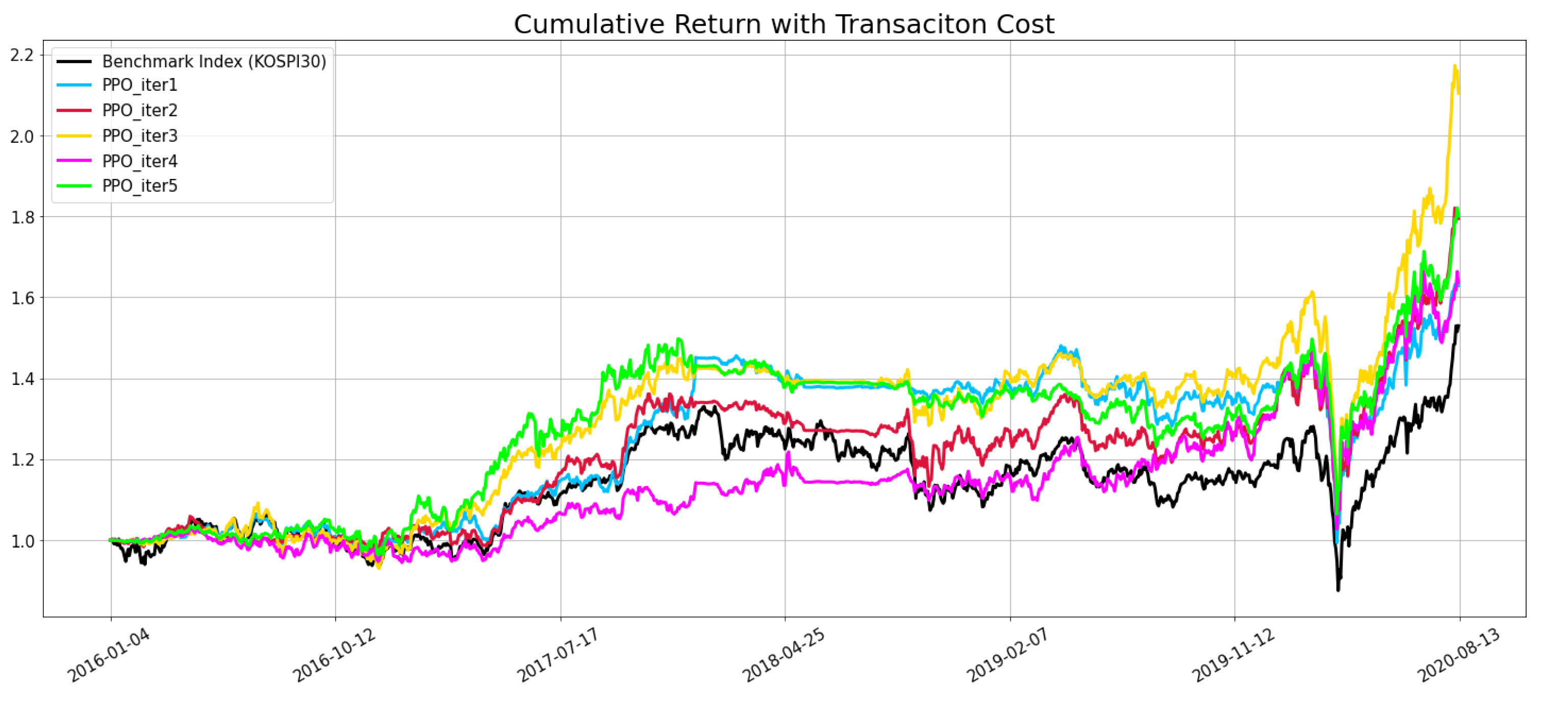We tested whether the model’s performance was enhanced by changing $h_{max}$, buying threshold, and selling threshold based on the PPO agent because the trading agent with the best average performance in the KOSPI market was PPO. The PPO agent obtained a higher cumulative return than the KOSPI30 in all five experimental iterations through the trading strategy changes. The values of $h_{max}$, buying threshold, and selling threshold were 10, 3, and 0, respectively, and the results are shown in Figure 7.

We extended the application of this trading strategy to A2C, DDPG, the ensemble strategy, and Remake Ensemble Trading agents and conducted five experiments, as in the case of PPO. As a result, the average performance of all agents was better than before the trading strategy adjustment, and overall performance was better for individual iterations. In particular, in the case of the ensemble strategy, similar to PPO, the cumulative return was higher than the benchmark index in all its periods, and the average performance was also the best of the five trading agents. Although limited to the KOSPI market, in the end, we successfully improved the model in a way that met both of the conditions of robustness that we thought of earlier.

Table 4. Performance evaluation comparison for five agents after changing the trading strategy in the KOSPI market from 4 January 2016 to 13 August 2020 (1134 days).

Iteration	KOSPI30	A2C	DDPG	PPO	Ensemble	Remake
1		18.735%	67.375%	62.823%	57.216%	78.989%
2		35.623%	32.835%	79.415%	99.814%	68.474%
3	52.946%	53.683%	86.469%	110.387%	93.249%	42.380%
4		65.347%	64.380%	63.718%	76.005%	106.056%
5		45.906%	51.989%	80.092%	97.341%	72.467%
mean		43.8595%	60.610%	79.287%	84.725%	72.673%

describes these results, and in cases where agents performed better than the KOSPI 30, the text is marked in bold.

We applied the same trading strategy to the Dow Jones 30 and JPX and compared the cumulative returns between each benchmark index and the trading agents. The results are shown in

Table 5. Performance evaluation comparison for five agents after changing the trading strategy in the Dow Jones 30 from 4 January 2016 to 6 July 2020 (1134 days).

Iteration	DJIA	A2C	DDPG	PPO	Ensemble	Remake
1		32.523%	31.964%	19.995%	33.369%	34.353%
2		35.266%	37.225%	31.06%	29.186%	34.696%
3	53.278%	30.141%	35.27%	25.378%	24.174%	25.987%
4		25.905%	24.637%	22.356%	28.856%	32.28%
5		34.604%	28.937%	18.523%	26.281%	39.01%
mean		31.688%	31.607%	23.462%	28.373%	33.265%

and

Table 6. Performance evaluation comparison for five agents after changing the trading strategy in the JPX market from 4 January 2016 to 21 July 2020 (1134 days).

Iteration	JPX30	A2C	DDPG	PPO	Ensemble	Remake
1		100.422%	96.477%	50.446%	77.599%	109.832%
2		84.178%	79.738%	58.264%	92.764%	57.523%
3	71.51%	110.631%	76.879%	54.933%	80.807%	82.248%
4		104.585%	90.693%	81.633%	79.084%	90.764%
5		61.004%	101.648%	45.742%	62.45%	65.715%
mean		92.164%	89.087%	58.204%	78.397%	81.216%

, respectively. As shown in Table 6, for JPX stocks, the new trading state showed good performance, as in the case of the KOSPI. In contrast, in the Dow Jones 30, unlike in the case of KOSPI, the new trading strategy significantly reduced all agents’ performance.

As mentioned earlier, the core of the new trading strategy is conservatism. Given that this strategy backfired in the Dow Jones 30 market, it can be assumed that aggressive trading strategies may be more effective in the Dow Jones 30 market. On the other hand, in the case of the JPX market, similar performance improvements to the KOSPI were made under the new trading strategy established based on the KOSPI. Thus it can be assumed that the JPX and KOSPI markets are almost identical, and the conservative approach is relatively practical. Of course, it can be seen that if we are to improve performance better than in the previous experiment, we need sophisticated and customized trading strategies for the Dow Jones 30 and JPX rather than the strategy tailored to the KOSPI, which sets $h_{max}$, buying threshold, and selling threshold to 10, 3, 0, respectively. Our experimental results are available on https://github.com/kongminseok/EAASTUDRL.

7. Conclusions and Future Work

In this paper, we empirically analyzed the performance of automated stock trading based on deep reinforcement learning through experiments to validate the contents of [10]. We conducted empirical analysis in three ways to determine whether it is possible to generalize automated stock trading, including several DRL-based trading agents. First, we added a new trading agent, which is named ’Remake Ensemble’, and it is based on the ensemble strategy. Since Remake Ensemble showed no significant performance difference compared to other agents, we concluded that adding several different DRL algorithms to the ensemble-based trading agent would make it difficult to increase the robustness of the model.

Furthermore, we expanded the trading model to the KOSPI and JPX markets for analysis and wondered if there was a way to increase the model’s performance in each market. As one of the methods, the trading strategy was changed to a more conservative and general form by adjusting several model hyperparameters. A new trading strategy was applied based on the KOSPI, which had the lowest performance.

Finally, by changing the trading strategy of the original model, we observed that the model’s robustness could be improved in the KOSPI and JPX markets. The average performance of all agents was better than before changing the trading strategy, and the whole performance was better for individual iterations. However, the performance was low when the same model was applied to the Dow Jones 30.

This empirical analysis is only one possible direction toward a robust automated stock trading system. It cannot be guaranteed that it is optimal for a more stable and robust model. If the experimental iteration exceeds five times, it is unknown whether the PPO and the ensemble strategy still guarantee a higher cumulative return than the KOSPI30 for all iterations. Further, there is no promise that the model will yield stable returns if the trading period or timing are changed.

Although it is clear that the ensemble strategy presented in [10] is a novel and innovative approach, we thought the automated stock trading system still had many potential improvements that have not yet been empirically demonstrated apart from the experiments we conducted. The key is generalization and higher profit. One of the methods related to generalization is the possibility of performance improvement in the Dow Jones 30 and JPX markets through customizing the trading strategy, as in the KOSPI market. Suppose it is possible ensuring a higher return than the benchmark index of the three markets. In that case, it can be challenging to make a general model guarantee stable returns in more diverse markets such as the S&P 500 and KOSDAQ. These things can be called market generalization. The other task is to create a model that assures higher profits than the benchmark index during all trading intervals in various markets. It can be called time generalization.

The original model verifies the agent’s performance based on the current SR, but other metrics such as CR can be used instead of the SR. In addition, a way to replace the turbulence threshold by reflecting rates such as the U.S. Federal Reserve’s interest rates in the environment may be a keyword for higher prediction and performance improvement. This idea is conceived based on the observation that the Fed’s recent rate hike and the financial market shrinkage were carried out in parallel. In addition to interest rates, major economic indicators such as oil prices and the consumer price index (CPI) can be used as components of the environment to train the model. Designing rewards more elaborately can also be a topic for future work.

References

1. Fischer, T.G. Reinforcement Learning in Financial Markets—A Survey; FAU Discussion Papers in Economics 12/2018; Friedrich-Alexander University Erlangen-Nuremberg, Institute for Economics: Erlangen, Germany, 2018. [Google Scholar]
2. Bekiros, S.D. Fuzzy adaptive decision-making for boundedly rational traders in speculative stock markets. Eur. J. Oper. Res. 2010, 202, 285–293. [Google Scholar] [CrossRef]
3. Zhang, Y.; Yang, X. Online Portfolio Selection Strategy Based on Combining Experts’ Advice. Comput. Econ. 2017, 50, 141–159. [Google Scholar] [CrossRef]
4. Kim, Y.; Ahn, W.; Oh, K.J.; Enke, D. An intelligent hybrid trading system for discovering trading rules for the futures market using rough sets and genetic algorithms. Appl. Soft Comput. 2017, 55, 127–140. [Google Scholar] [CrossRef]
5. Rubinstein, M. Markowitz’s “Portfolio Selection”: A Fifty-Year Retrospective. J. Financ. 2002, 57, 1041–1045. [Google Scholar] [CrossRef] [Green Version]
6. Bertsekas, D.P. Dynamic Programming and Optimal Control, 3rd ed.; Athena Scientific: Belmont, MA, USA, 2005; Volume I. [Google Scholar]
7. Bertoluzzo, F.; Corazza, M. Testing Different Reinforcement Learning Configurations for Financial Trading: Introduction and Applications. Procedia Econ. Financ. 2012, 3, 68–77. [Google Scholar] [CrossRef]
8. Neuneier, R. Optimal Asset Allocation using Adaptive Dynamic Programming. In Proceedings of the Advances in Neural Information Processing Systems; Touretzky, D., Mozer, M., Hasselmo, M., Eds.; MIT Press: Cambridge, MA, USA, 1995; Volume 8. [Google Scholar]
9. Neuneier, R. Enhancing Q-Learning for Optimal Asset Allocation. In Proceedings of the Advances in Neural Information Processing Systems; Jordan, M., Kearns, M., Solla, S., Eds.; MIT Press: Cambridge, MA, USA, 1997; Volume 10. [Google Scholar]
10. Yang, H.; Liu, X.; Zhong, S.; Walid, A. Deep reinforcement learning for automated stock trading: An ensemble strategy. In Proceedings of the ICAIF ’20: The First ACM International Conference on AI in Finance, New York, NY, USA, 15–16 October 2020; pp. 31:1–31:8. [Google Scholar] [CrossRef]
11. Konda, V.; Tsitsiklis, J. Actor-Critic Algorithms. In Proceedings of the Advances in Neural Information Processing Systems; Solla, S., Leen, T., Müller, K., Eds.; MIT Press: Cambridge, MA, USA, 1999; Volume 12. [Google Scholar]
12. Mnih, V.; Badia, A.P.; Mirza, M.; Graves, A.; Lillicrap, T.P.; Harley, T.; Silver, D.; Kavukcuoglu, K. Asynchronous Methods for Deep Reinforcement Learning. CoRR 2016, arXiv:1602.01783. [Google Scholar]
13. Zhang, Z.; Zohren, S.; Roberts, S. Deep Reinforcement Learning for Trading. arXiv 2019, arXiv:1911.10107. [Google Scholar] [CrossRef]
14. Lillicrap, T.P.; Hunt, J.J.; Pritzel, A.; Heess, N.; Erez, T.; Tassa, Y.; Silver, D.; Wierstra, D. Continuous control with deep reinforcement learning. arXiv 2015, arXiv:1509.02971. [Google Scholar] [CrossRef]
15. Liang, Z.; Chen, H.; Zhu, J.; Jiang, K.; Li, Y. Adversarial Deep Reinforcement Learning in Portfolio Management. arXiv 2018, arXiv:1808.09940. [Google Scholar] [CrossRef]
16. Xiong, Z.; Liu, X.; Zhong, S.; Yang, H.; Walid, A. Practical Deep Reinforcement Learning Approach for Stock Trading. CoRR 2018, arXiv:1811.07522. [Google Scholar]
17. Schulman, J.; Wolski, F.; Dhariwal, P.; Radford, A.; Klimov, O. Proximal Policy Optimization Algorithms. CoRR 2017, arXiv:1707.06347. [Google Scholar]
18. Lei, C. Deep reinforcement learning. In Deep Learning and Practice with MindSpore; Springer: Berlin/Heidelberg, Germany, 2021; pp. 217–243. [Google Scholar]
19. Luenberger, D.G. Investment Science; Oxford University Press: Oxford, UK, 1997. [Google Scholar]
20. Hull, J. Options, Futures, and Other Derivatives, 6th ed.; Pearson Internat, Ed.; Pearson Prentice Hall: Upper Saddle River, NJ, USA, 2006. [Google Scholar]
21. Li, Y. Deep Reinforcement Learning: An Overview. CoRR 2017, arXiv:1701.07274. [Google Scholar]
22. Glasserman, P. Monte Carlo Methods in Financial Engineering; Springer: New York, NY, USA, 2004. [Google Scholar]
23. Longstaff, F.; Schwartz, E. Valuing American Options by Simulation: A Simple Least-Squares Approach. Rev. Financ. Stud. 2001, 14, 113–147. [Google Scholar] [CrossRef]
24. Tsitsiklis, J.; Van Roy, B. Regression methods for pricing complex American-style options. IEEE Trans. Neural Netw. 2001, 12, 694–703. [Google Scholar] [CrossRef] [PubMed] [Green Version]
25. Li, Y.; Szepesvári, C.; Schuurmans, D. Learning Exercise Policies for American Options. In Proceedings of the Twelfth International Conference on Artificial Intelligence and Statistics, AISTATS 2009, Clearwater Beach, FL, USA, 16–18 April 2009. [Google Scholar]
26. Pastor, L.; Stambaugh, R.F. Predictive Systems: Living with Imperfect Predictors; Working Paper 12814; National Bureau of Economic Research: Cambridge, MA, USA, 2007. [Google Scholar] [CrossRef]
27. Viceira, L.; Luis, M.; Viceira, J.; Campbell, J.; Viceira, L.; Campbell, O.; Press, O.U.; Viceira, L. Strategic Asset Allocation: Portfolio Choice for Long-Term Investors; Clarendon Lectures in Economics; Oxford University Press: Oxford, UK, 2002. [Google Scholar]
28. Brandt, M.W.; Goyal, A.; Santa-Clara, P.; Stroud, J.R. A Simulation Approach to Dynamic Portfolio Choice with an Application to Learning About Return Predictability. Rev. Financ. Stud. 2005, 18, 831–873. [Google Scholar] [CrossRef] [Green Version]
29. Moody, J.; Saffell, M. Learning to trade via direct reinforcement. IEEE Trans. Neural Netw. 2001, 12, 875–889. [Google Scholar] [CrossRef] [Green Version]
30. Deng, Y.; Bao, F.; Kong, Y.; Ren, Z.; Dai, Q. Deep Direct Reinforcement Learning for Financial Signal Representation and Trading. IEEE Trans. Neural Netw. Learn. Syst. 2017, 28, 653–664. [Google Scholar] [CrossRef]
31. Chen, L.; Gao, Q. Application of Deep Reinforcement Learning on Automated Stock Trading. In Proceedings of the 2019 IEEE 10th International Conference on Software Engineering and Service Science (ICSESS), Beijing, China, 18–20 October 2019; pp. 29–33. [Google Scholar] [CrossRef]
32. Dang, Q. Reinforcement Learning in Stock Trading. In Advanced Computational Methods for Knowledge Engineering—Proceedings of the 6th International Conference on Computer Science, Applied Mathematics and Applications, ICCSAMA 2019, Hanoi, Vietnam, 19–20 December 2019; Thi, H.A.L., Le, H.M., Dinh, T.P., Nguyen, N.T., Eds.; Advances in Intelligent Systems and Computing; Springer: Berlin/Heidelberg, Germany, 2019; Volume 1121, pp. 311–322. [Google Scholar] [CrossRef] [Green Version]
33. Jeong, G.; Kim, H.Y. Improving financial trading decisions using deep Q-learning: Predicting the number of shares, action strategies, and transfer learning. Expert Syst. Appl. 2019, 117, 125–138. [Google Scholar] [CrossRef]
34. Jiang, Z.; Liang, J. Cryptocurrency Portfolio Management with Deep Reinforcement Learning. CoRR 2016, arXiv:1612.01277. [Google Scholar]
35. Bekiros, S.D. Heterogeneous trading strategies with adaptive fuzzy Actor–Critic reinforcement learning: A behavioral approach. J. Econ. Dyn. Control 2010, 34, 1153–1170. [Google Scholar] [CrossRef]
36. Li, J.; Rao, R.; Shi, J. Learning to Trade with Deep Actor Critic Methods. In Proceedings of the 11th International Symposium on Computational Intelligence and Design, ISCID 2018, Hangzhou, China, 8–9 December 2018; Volume 2, pp. 66–71. [Google Scholar] [CrossRef]
37. Chakole, J.B.; Kolhe, M.S.; Mahapurush, G.D.; Yadav, A.; Kurhekar, M.P. A Q-learning agent for automated trading in equity stock markets. Expert Syst. Appl. 2021, 163, 113761. [Google Scholar] [CrossRef]
38. Subramanian, H.; Ramamoorthy, S.; Stone, P.; Kuipers, B.J. Designing Safe, Profitable Automated Stock Trading Agents Using Evolutionary Algorithms. In Proceedings of the 8th Annual Conference on Genetic and Evolutionary Computation; Association for Computing Machinery, New York, NY, USA, 1 January 2006; pp. 1777–1784. [Google Scholar] [CrossRef] [Green Version]
39. Bhat, A.A.; Kamath, S.S. Automated stock price prediction and trading framework for Nifty intraday trading. In Proceedings of the 2013 Forth International Conference on Computing, Communications and Networking Technologies (ICCCNT), Tiruchengode, India, 4–6 July 2013; pp. 1–6. [Google Scholar] [CrossRef]
40. Fama, E. Efficient Capital Markets: A Review of Theory and Empirical Work. J. Financ. 1970, 25, 383–417. [Google Scholar] [CrossRef]
41. Chong, T.T.L.; Ng, W.K.; Liew, V.K.S. Revisiting the Performance of MACD and RSI Oscillators. J. Risk Financ. Manag. 2014, 7, 1–12. [Google Scholar] [CrossRef] [Green Version]
42. Cohen, G.; Qadan, M. The Complexity of Cryptocurrencies Algorithmic Trading. Mathematics 2022, 10, 2037. [Google Scholar] [CrossRef]
43. Mndawe, S.T.; Paul, B.S.; Doorsamy, W. Development of a Stock Price Prediction Framework for Intelligent Media and Technical Analysis. Appl. Sci. 2022, 12, 719. [Google Scholar] [CrossRef]
44. Maitah, M.; Procházka, P.; Čermák, M.; Šrédl, K. Commodity Channel Index: Evaluation of Trading Rule of Agricultural Commodities. Int. J. Econ. Financ. Issues 2016, 6, 176–178. [Google Scholar]
45. Gurrib, I. Performance of the Average Directional Index as a market timing tool for the most actively traded USD based currency pairs. Banks Bank Syst. 2018, 13, 58–70. [Google Scholar] [CrossRef]
46. Sharpe, W.F. The Sharpe Ratio. J. Portf. Manag. 1994, 21, 49–58. [Google Scholar] [CrossRef] [Green Version]
47. Kritzman, M.; Li, Y. Skulls, Financial Turbulence, and Risk Management. Financ. Anal. J. 2010, 66, 30–41. [Google Scholar] [CrossRef]
Figure 1. Agent–environment interface.
Applsci 13 00633 g001
Figure 2. Stock Trading Mechanism Overview.
Applsci 13 00633 g002
Figure 3. Cumulative returns for each agent with the DJIA (the dotted line is the benchmark index, which is the cumulative return of the DJIA).
Applsci 13 00633 g003
Figure 4. Cumulative returns of each agent with the average return of the top 30 KOSPI stocks (the dotted line is the benchmark index, which is the cumulative return of the KOSPI30).
Applsci 13 00633 g004
Figure 5. Cumulative returns of each agent with the average return of the top 30 JPX stocks (the dotted line is the benchmark index, which is the cumulative return of the JPX30).
Applsci 13 00633 g005
Figure 6. Cumulative return curves of the original ensemble strategy agent and DJIA ( h m a x = 100 , buying threshold = 0, selling threshold = 0, initial portfolio value $1,000,000, from 4 January 2016 to 6 July 2020, (1134 days)).
Applsci 13 00633 g006
Figure 7. Cumulative return curves of PPO agent and KOSPI30 ( h m a x = 10 , buying threshold = 3, selling threshold = 0, initial portfolio value 1,000,000,000, from 4 January 2016 to 13 August 2020 (1134 days)).
Applsci 13 00633 g007