Article

Two-Stage Tour Route Recommendation Approach by Integrating Crowd Dynamics Derived from Mobile Tracking Data

State Key Laboratory of Information Engineering in Surveying, Mapping and Remote Sensing, Wuhan University, Wuhan 430079, China
*
Author to whom correspondence should be addressed.
Appl. Sci. 2023, 13(1), 596; https://doi.org/10.3390/app13010596
Submission received: 14 November 2022 / Revised: 13 December 2022 / Accepted: 26 December 2022 / Published: 1 January 2023
(This article belongs to the Special Issue State of the Art in Recommendation and Mobile Systems for Tourism)

Abstract

:
Tourism activities essentially represent the interaction between crowds and attractions. Thus, crowd dynamics are critical to the quality of the tourism experience in personalized tour recommendations. In order to generate dynamic, personalized tour routes, this paper develops a tourist trip design problem with crowd dynamics (TTDP-CD), which is quantified with the crowd dynamics indicators derived from mobile tracking data in terms of crowd flow, crowd interaction, and crowd structure. TTDP-CD attempts to minimize the perceived crowding and maximize the assessed value of destinations while minimizing the total distance and proposes a two-stage route strategy of “global optimization first, local update later” to deal with the sudden increase in crowding in realistic scenarios. An evolutionary algorithm is extended with container-index coding, mixed mutation operators, and a global archive to create a personalized day tour route at the urban scale. To corroborate the performance of this approach, a case study was carried out in Dalian, China. The results demonstrate that the suggested method outperforms previous approaches, such as NSGA-II, MOPSO, MOACO, and WSM, in terms of performance and solution quality and decreases real-time crowding by an average of 7%.

1. Introduction

The tourist trip design problem (TTDP) is the core problem of the tourism recommendation system (TRS). It is used to solve the challenges of information overload and decision-making difficulties for tourists, which involves the time allocation at a point of interest (POI) and the spatial structures of the routes (including POI selection and sequencing) [1,2,3,4,5]. A solution of a TTDP aims to find optimal routes to maximize the obtained utility (e.g., score, profit) [4,6,7,8] and minimize the cost (e.g., distance, expense) [9,10], which improves the tourism experience while accounting for various constraints (e.g., time budget and personal preferences) [11].
Tourism experience is essential and necessary for tour route recommendations and is complex due to its multi-faceted nature, tourists’ mobile nature, and uncertainty in tourism destinations [12]. In addition to facilities and services, attractions’ crowding situation significantly impacts the tourist experience, as “over-tourism” can negatively affect visitors’ perceptions of crowding, resulting in lower customer satisfaction and revisit rates [5,13,14]. For instance, the current crowding-related TTDP is limited to the interiors of specific attractions and lacks the co-analysis of the crowding of multiple attractions. In addition, few studies have focused on coping with the sudden increase in crowds, and a dynamic adjustment mechanism and attraction replacement strategy are urgently required in route recommendation [11,15,16]. In addition, the tourism value is essential for determining whether an attraction is worth visiting and is ordinarily measured and rated objectively with the ranking of facilities and services. However, the recommendations made often ignore the current trending and tourists’ selection behaviors. Notably, supercities (cities with a permanent population of 5 to 10 million) are rich in tourism resources, representing a vast number of attractions and a wider geographical spread, making them popular destinations for many tourists. Apparently, it is quite difficult for those tourists with limited knowledge about the destinations and current trends to choose attractions and plan routes in the supercity. Furthermore, the expansion of the city scale poses a significant challenge to the data source’s applicability, the model’s practicality, and the algorithm’s capability in TTDP.
To cope with these gaps, crowd dynamics derived from broad-coverage mobile tracking data, which refer to the quantitative descriptions of the movement of humans in space and time, are feasibly capable of evaluating the value of attractions in the supercity and managing crowding. Mapping tourist movements gives an understanding of tourism destinations and the interconnections between destinations [17,18]. For example, capturing tourists’ mobility (e.g., distribution of the duration of stay per attraction and which attractions are frequently visited together) and social connections (e.g., identifying similar users with spatial co-occurrences) are helpful in ranking and composing the itinerary [19]. With crowd dynamics information, the tourism experience quality of the TTDP could be further improved.
The contribution of this paper can be summarized as follows. First, this paper defines a tourist trip design problem with crowd dynamics (TTDP-CD) for the first time in literature and proposes an effective two-stage route strategy of “global optimization first, local update later” to generate dynamic, personalized tour routes with less crowded situations, including initial pre-tour itineraries and dynamically adjusted in-tour itineraries for avoiding sudden overcrowding. Second, the crowd dynamics indicators (i.e., crowd flow, crowd interaction, and crowd structure) are derived from mobile tracking data to support the construction of two-stage multi-objective model in terms of three conflicting objectives (i.e., crowding, value, and distance) and dynamic adjustment strategy. These indicators describe the characteristics of attractions as affected by human tourism mobilities in space and time. Third, an improved non-dominated sorting genetic algorithm II (INSGA-II) with container-index coding, mixed mutation operators, and an archiving strategy is proposed to solve TTDP-CD. It overcomes the difficulties in the conflicting objectives and multiple constraints involved with time-varying crowding, attraction selection, sequence determination, and time allocation, particularly in supercities.
This paper carries out a case in Dalian, China, to evaluate the performance of the proposed strategies and methods. The comparison of performance and evaluation of solutions demonstrates that the INSGA-II outperforms other approaches. In addition, combining the initial route with dynamic adjustment, the proposed two-stage strategy can offer tourists a dynamic, less-crowded tour route in the supercity with high immediacy and low adjustment costs.
The remaining sections of this paper are structured as follows. Section 2 comprehensively reviews the related works. Section 3 describes the methodology for solving TTDP-CD, including data processing, index deriving, model construction, and algorithm operation. Section 4 presents a case study conducted in Dalian. Section 5 evaluates the performance of our proposed approach and strategy. Finally, Section 6 provides conclusions and suggestions for future research directions.

2. Literature Review

2.1. Tourist Trip Design Problem

Personalized tour itineraries have replaced standard tour packages as the norm in travel planning [20,21]. TRSs are committed to meeting individual travel requirements and helping to organize leisure and travel plans. The emphasis of TRS research is now shifting to recommendations for complete travel itineraries, which can be addressed by solving the TTDP [19]. The existing research has led to tremendous advances in the model and algorithm design of TTDP.
TTDP variants can be categorized as either single-tour or multiple-tour variants [22]. The orienteering problem (OP) is the basis for modeling the single-tour TTDP, aiming to maximize the overall profit obtained while adhering to time and budget constraints [23]. Several extensions of OP, such as the orienteering problem with time windows (OPTW) [24] and the time-dependent orienteering problem (TDOP) [25], have been successfully applied to model complex versions of single-tour TTDP. Multiple-tour TTDP can be modeled as a vehicle routing problem with profits (VRPP) in which profits are distributed across multiple vehicles with a limited capacity [26].
The objectives in TTDP can be summarized as maximizing profit, minimizing cost, and customized objectives. Profit gained from visiting POIs, such as the total score and utility of attractions, should be maximized [7,27,28]. Minimizing costs can be reflected in minimizing the distance [29] and expenses [30]. Moreover, customized objectives are designed to solve specific application-related problems. For instance, Divsalar et al. (2022) [30] included minimizing total emissions from travel as one of the TTDP’s green travel goals.
Concerning the algorithms for solving TTDP, exact and meta-heuristic methods are typically employed. In the exact algorithm field, methods such as the weighted-sum method and mixed-integer linear programming are generally applied, which can transform multi-objective problems into single-objective problems. In relation to meta-heuristic algorithms, single-solution-based and population-based metaheuristics are commonly-used approaches [31]. Single-solution-based metaheuristics include local search, tabu search, and simulated annealing [21,27,30,32]. Evolutionary algorithms (e.g., genetic algorithms, evolutionary strategies) and swarm intelligence-based methods (e.g., ant colony, particle swarm optimization) [6,33,34] are examples of population-based metaheuristics. Typically, a multi-objective problem is resolved by augmenting the metaheuristic algorithm with specific search components, such as fitness assignment, diversity preservation, and elitism.
As research in TTDP flourishes, the theories and methods applied to TTDP are used in various intelligent tools, such as digital applications and e-guides [35]. Specifically, several mobile and web-based decision support applications that facilitate tourism have been introduced. Gavalas et al. [36] employed a metaheuristic based on a local search, namely the SlackRoutes, to solve the TTDP and developed a web and mobile client application, eCOMPASS, to help users to plan their multi-day tours by providing them with the specific route, time schedule, and transportation mode. Kurata et al. [37] introduced a user-friendly web-based tour planning application, CT-Planner4 (https://ctplanner.jp/ctp5/, accessed on 5 December 2022), where the user can select the target area, mode of transport, starting point, end point, and travel style on the web page and then acquire the planned route visualized on an online map.
The above TTDP-related works focus more on the profit and utility tourists attained from attractions and give less attention to how the crowd movements of tourists influence the attraction characteristics dynamically. These crowd dynamics contain a wealth of information that can help to understand the attractions better and enhance the tourism experience. For this reason, we propose a framework of the TTDP-CD to meet the actual application requirements, which appears for the first time in the literature.

2.2. Crowd Dynamics in Tourism

Crowd dynamics refer to the quantitative descriptions of the movement of humans in space and time, which are widely employed in urban planning and tourism to comprehend the movement of individuals [38]. Common statistical approaches to crowd dynamics include quantitative statistical analysis of flow, interaction network analysis, and the calculation of mobility indicator values [39,40,41].
Crowd dynamics can enhance the tourism experience in TTDP in numerous ways, such as preventing congestion and enhancing destination awareness. Nowadays, academic interest is gradually growing in crowd-aware TTDP. Various studies have demonstrated that large crowds within an attraction indicate the attraction’s popularity and create a more enjoyable entertainment atmosphere [42,43,44]. However, “over-tourism” caused by excessive crowds poses significant safety risks, especially in the post-COVID-19 phase, when visitors become more sensitive to crowding and avoid crowded places voluntarily in the short term [45]. Some researchers have considered attraction congestion as an objective of the TTDP. Wang et al. (2016) [34] constructed a multi-objective time-varying function that incorporated POI heat, user interest, and crowding data, and solved the problem by employing a variant of the ant colony optimization algorithm to provide users with a travel itinerary that avoids the most crowded time of the POI. In addition to the congestion, the interactive network of attractions constructed by tourists’ mobility contains a wealth of information that can be used for destination comprehension. For instance, in the destination network, a high degree of centrality indicates higher power and status of the nodes [40,46]. Lastly, the composition of the population structure of attractions can be used to describe the audience type of the attraction quantitatively. It can be used for substitution between attractions, which is inspired by the concept of homophily [39,47]. However, existing studies have not explored crowds, and there is no practical method to adjust tourist routes to address sudden crowd surges.
There are various data sources for obtaining crowd dynamics. RFID, GPS chip-embedded tickets, and pedestrian sensors can be utilized to obtain crowding data at attractions [34,48,49]. Information on past tour behaviors requires access to the complete travel chain of visitors in the city, which can be collected from social media data and web notes [40,50]. However, those geo-tag data are highly biased and hardly reflect the travel activities of the vast remaining majority of those who do not post online. With the widespread penetration of smart tourism in tourism activities, big data, such as mobile tracking data, is increasingly used in the studies of tourism activities [51,52,53,54]. Compared to existing data sources, mobile tracking data provides a larger volume, more comprehensive, and boarder description of travel flows [55]. However, research on using mobile tracking data to aid TTDP has not yet been proposed to the best of our knowledge.
In this work, a novel framework for modeling and solving the Tourist Trip Design Problem with Crowd Dynamics is designed to recommend personalized, dynamic one-day tours in supercities, using broad-coverage mobile tracking data and an improved multi-objective algorithm. The two-stage strategy brings the dynamic TTDP to the front, providing the adjustment solution when faced with emergencies such as overcrowding.

3. Methodology

3.1. Research Framework and Definitions for TTDP-CD

This paper proposes a novel research framework for solving TTDP-CD, shown in Figure 1, for generating personalized, dynamic one-day tour routes with a high experience value for the tourists. We divided the research process into four sections. (1) Data processing. A massive amount of mobile tracking data with rich location and time information is used as the data source to extract past tourist trips, which are represented by tourism activity chains. (2) Indices derivation. Tourism activity chains are used to derive indicators of three types of crowd dynamics, including crowd flow, crowd interaction, and crowd structure. (3) Model construction. With the derived crowd dynamics indicators, this study defines three objectives, including minimizing crowding, maximizing value, and minimizing distance, with multiple constraints and employing a two-stage route strategy for generating initial pre-tour routes and dynamically adjusted in-tour itineraries to avoid sudden overcrowding. (4) Algorithm operation. The constructed multi-objective model is solved with a heuristic algorithm, INSGA-II, both in the pre-tour initial routing stage and in-tour dynamic adjustment stage, thus generating the initial pre-tour routes and the adjusted in-tour routes.
The proposed TTDP-CD is novel in terms of model and algorithm. Unlike the traditional TTDP model, the TTDP-CD applies the crowd dynamics patterns obtained from past tourist trips to tourist itinerary planning for the first time in the literature, as reflected in the avoidance of peak crowds, attraction scores with reference to realistic choices, and adaptive in-tour dynamic adjustments under unexpected circumstances. These improvements can not only lead to better tourist experiences and more flexible itineraries in realistic and unexpected situations, but also provide a novel perspective on the application of crowd dynamics in tourism research. As an optimization problem in mathematics, TTDP is commonly solved by employing meta-heuristic algorithms. Among them, the evolutionary algorithms augmented with specific search components, such as NSGA-II, are commonly used to solve multi-objective problems. Our INSGA-II is further improved based on NSGA-II from the aspects of chromosome coding, mutation operation, and evolving strategy to overcome the difficulties in route planning in supercities, thus generating better Pareto solutions of the recommended routes.
Definition 1 (Attraction Network).
The attraction network G = A , E , W is constructed with all attractions in the city, where A is a set of attraction vertices. The edge E represents the directed transfer between vertices, whose weight consists of two attributes of distance travelled and time spent on the transfer, and W = ( d i j , t i j ) i , j A , i j . A i denotes a tourism attraction, and i = 1, 2, …, N A , where N A denotes the total number of attractions. For a more realistic route, the elements in weight W are obtained via the Baidu Map API (https://lbsyun.baidu.com) which can provide the optimal path between the determined departure and destination locations for various transportation modes. In this study, the transportation mode between attractions (walking or driving) is determined by the distance of each attraction transfer. The walking mode is employed if the distance is less than 1.5 km; otherwise, the driving mode is employed.
Definition 2 (Tourist preference weight).
Different tourists have different preferences. A tourist’ preference is represented by category preference weight [ α n , α c , α e ], where α n , α c , and α e denote the tourist’s desirability for natural landscapes, cultural sightseeing, and entertainment attractions, and α n + α c + α e = 1 .
Definition 3 (Time window).
Crowd dynamics indicators are time-varying. In this paper, the fifteen hours from 7 A.M. to 10 P.M. are divided into several time windows at different time intervals. W k denotes the k-th time window at a three hours interval with k = 1, 2, …, 5, while w k at one hour interval with k = 1, 2, …, 15.

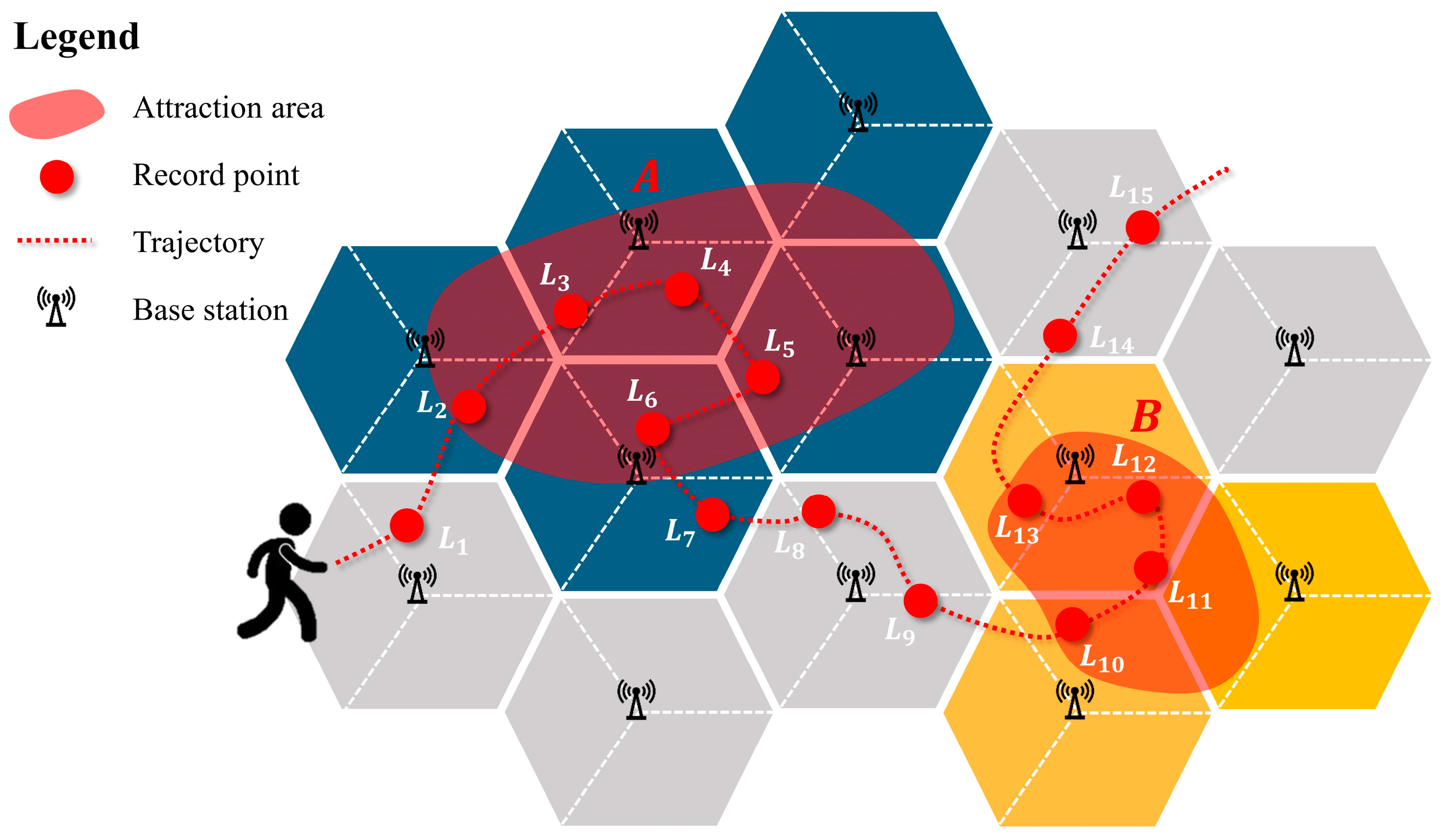
3.2. Data Processing: Generating Tourism Activity Chains

The broad coverage and low acquisition cost of mobile tracking data allow for an accurate description of tourism activities from individual and group perspectives [56]. As depicted in Figure 2, a user’s travel trajectory is recorded as the cell phone signal communicates with the base station. With the correspondence between the attraction area and base station location determined, the user’s stay within the attractions can be detected. Our goal is to identify tourists’ stays at multiple attractions within the city, thereby constituting complete tourism activity chains. First, the raw mobile tracking data needs to be preprocessed. Second, generate the stay sequences in attractions with mobile tracking data. Lastly, identify tourists with a filtering strategy based on the tourists’ spatiotemporal behaviors and generate tourism activity chains. Any users who meet the following spatiotemporal behaviors criteria are detected as tourists: (1) users who access the attraction area during the opening hours and spend more than 30 min there; (2) users who stay overnight (0 A.M. to 6 A.M.) at the same attraction or visit the attraction three or more times in a single day are judged to be the residents in the attraction area, not tourists; (3) users who stay at the same attraction during the daytime (8 A.M. to 7 P.M.) with several staying days more than half of the days of interest are judged to be commuters in the attraction area, not tourists.
After completing the above processes, tourism activity chains are extracted. A tourist’s tourism activity chain is represented as the following list: C = P 1 , T 1 s , T 1 e , P 2 , T 2 s , T 2 e , , P n , T n s , T n e , where P i denotes the i-th tourism attraction in the chain, while T i s and T i e denote the starting and ending time of the visit to P i .

3.3. Indices Deriving: Calculating Crowd Dynamics Indicators

Crowd dynamics indicators describe the characteristics of attractions as affected by human movements in tourism, and provide the source data for route design and adjustment. Based on previous research and the impact of crowd mobility on the tourism experience, this paper derives three crowd dynamics indicators of each attraction from the tourism activity chains: (1) crowd flow indicator (relative crowding at the attraction); (2) crowd interaction indicators (degree of centrality in the crowd interaction network of attractions); (3) crowd structure indicators (similarity of crowd structure between attractions).
  • Crowd Flow Indicator. To some extent, the crowding of attractions represents a higher popularity and a more entertaining atmosphere; however, “over-tourism” poses more significant security risks and reduces the quality of the tourism experience. Since the congestion at each attraction has time-period regularity, the crowding experienced on the tour can be reduced by avoiding the peak hours at each attraction. The crowd flow indicator ( F ¯ i , w k ) represents the average relative crowding between different days in the same time window, which is calculated as follows:
    F ¯ i , w k = 1 N D D = 1 N D f l o w i , D , w k M A X ( f l o w i )
    where f l o w i , D , w k denotes the number of tourists at A i within time window w k of day D; M A X ( f l o w i ) denotes the maximum number of tourists at A i in all time windows over several days; N D is the total number of days.
  • Crowd Interaction Indicator. Crowd interaction refers to the movement of crowds between attractions resulting from the transformation of tourists. The directed crowd interactive network of attractions in different time windows is constructed by calculating the number of transfers between attractions with the tourism activity chains of all tourists, which are used as the weight of edges. In the interaction network, the nodes with a higher degree centrality have higher significance and status. The in-degree and out-degree of centrality of the node in different time windows can be calculated as follows:
    D i , i n , W k = j N A r i j , i n , W k
    D i , o u t , W k = j N A r i j , o u t , W k
    where r i j , i n , W k is the number of tourists from attraction A i to A j in time window W k ; r i j , o u t , w k is the number of tourists from A j to A i in W k .
  • Crowd Structure Indicator. The tourism behavioral characteristics of tourists can reflect the characteristics of the target audience of the attraction, which can be obtained from the tourism activity chains, listed as follows. (1) duration of stay at an attraction ( D A ); (2) average ticket expense per day ( E A v g ); (3) average number of attractions per day ( N A v g ); (4) average duration of stay per attraction ( D A v g ); (5) number of days to play ( D T ); (6) activity entropy ( A e ); (7) radius of gyration ( R g ). Activity entropy measures the diversity of an individual’s mobility behavior [57]:
    A e = i = 1 N A p i log p i
    where p i is the proportion of stay time at attraction A i . A larger value for A e implies the tourist has a higher diversity of activities. Radius of gyration is commonly used to evaluate the spatial dispersion of an individual’s movement [58]:
    R g = i = 1 N A ( l i l c ) 2 N A
    where l i denotes the x, y coordinates vector of A i ; l c = i = 1 N A l i / N A , which refers to the center of all the location of tourism attractions in the tourist’s tourism activity chain. A large value for R g reveals that the tourist is willing to travel in a large space. Thus, a tourist’s tourism behavioral characteristics can be denoted as a tuple: D A , E A v g , N A v g , D A v g , D T , A e , R g . Then, these behavior characteristics are divided into independent bins according to deciles and data characteristics, with the detailed dividing points are listed in Table A1 in the Appendix A. The crowd structure indicator C S I W k describes the proportional population structure of tourists with varying behavioural characteristics at an attraction, which is denoted C S I W k = P D A , P E A v g , P N A v g , P D A v g , P D T , P A e , P R g . Each element in C S I W k is a list detailing the proportion of tourists in each interval bin. Consequently, the similarity of crowd structure between attraction A and B in time window W k can be calculated as follows:
    S C S I , W k A , B = 1 i = 1 N C S I S E D ( p A , i , p B , i ) N C S I
    where p A , i and p B , i denote the tourist proportion of the i-th element in C S I W k of attraction A and B; S E D ( p A , i , p B , i ) denotes the squared Euclidean distance between the proportions; N C S I denotes the elements of C S I W k , and N C S I = 7 . The larger the value for S C S I , W k is, the more similar the crowd structure of the two attractions is, indicating that their audience groups are more similar. Therefore, the similarity relationship between attractions can serve as a reference for attraction substitution.

3.4. Model Construction: Two-Stage Multi-Objective Model for TTDP-CD

3.4.1. Model Objectives

As stated in the preceding section, this study aims to design personalized tour routes with a high level of experience value for tourists. The spatial structure of the route is optimized based on the multi-objective orienteering problem with time windows (MOOPTW) model, balancing the total crowding, value, and distance within a given time budget ( T m a x ).
The perceived crowding at each attraction depends on the crowding at the visiting time and the length of stay. With the tourist’s visiting time determined, the total perceived crowding during the tourist’s stay in A i , denoted as T P C i , can be defined as:
T P C i = w k W t i , w k · F ¯ i , w k / t i s
where t i , w k denotes the stay time in time windows w k ; F ¯ i , w k is the crowd flow indicator; t i s is the total stay time in A i .
To meet the tourist’s personalized preferences, the stay time in attraction A i , denoted as t i s , is adjusted from the historical average stay time t i based on the tourist’s preference for the category of A i . The tourist’s stay time at A i , denoted as t i s , is calculated as follows:
t = λ ( α i α n + α c + α e N t )
t i s = t i + t
where α i denotes the tourist’s preference for the category of A i , which is an element of tourist preference weight; λ denote the adjustment scaling factor; N t denotes the number of categories, and N t = 3 .
Generally, the value of an attraction is affected by objective factors (e.g., the attraction’s grade G i ) and subjective factors (e.g., the tourist’s preference α i ). The attraction’s grade reflects the quality of the landscape, environment, and service. There are five grades, including 5A, 4A, 3A, 2A, and no grade, corresponding to G i = 5 , 4 , 3 , 2 , 1 , respectively, according to the official standard of rating for the quality of tourist attractions in China. As for the preference, numerous studies have demonstrated that a tourist’s preference for a POI can significantly affect the value obtained at that particular POI [59,60]. In addition to grade and preference, visitors’ historical travel patterns are also substantially informative for determining the value of attractions. The attraction’s status value ( S i ) out of the attractions in the city can be reflected with its degree of centrality ( D i , i n and D i , o u t ) as crowd interaction indicator and denoted as Equation (10). A higher status value indicates greater importance of the attraction node, such as a core transit attraction [40,46]. Moreover, the average stay time ( t i ) in the attraction A i can reflect the value of A i . The more extended the stay at the attraction, the more appealing and worthwhile the attraction is. Therefore, the comprehensive value of attractions can be expressed as Equation (11), where β denotes a constant scaling factor and e represents the natural logarithm.
S i = D i , i n + D i , o u t
V i = β · G i · S i · t i · e α i
TTDP-CD’s objectives include minimizing the perceived crowding at the attractions along the itinerary (Equation (12)), maximizing the total value of the attractions in the itinerary (Equation (13)), and minimizing the total distance travelled, with the departure and final arrival locations determined by tourists (Equation (14)). To facilitate the calculation, the maximization objective function of value is converted into a minimization one by evaluating the opposite number.
min C =   i = 1 N A T P C i · x i
min   V = i = 1 N A V i · x i
min D =   i = 1 N A j = 1 N A d i j x i j + d 0 s + d 0 e
where x i is a discrete variable that takes a value of 0 or 1; if A i is visited in the itinerary, then x i = 1 ; otherwise, x i = 0 . In Equation (14), x i j is used to record the visiting sequence; x i j = 1 indicates that there is a sub-route of A i A j ; otherwise, x i j = 0 . d i j represents the distance from A i to A j . d 0 s and d 0 e indicate the distance from the departure location to the first attraction and from the last attraction to the final arrival location, respectively. The departure and final arrival location might be home or a hotel, as determined by the tourists’ individual preferences.

3.4.2. Model Constraints

There are two categories of model constraints: permanent technical constraints and customized constraints. As demonstrated by Equations (15)–(18), permanent technical constraints guarantee that designed routes are rational and valid [4]. Equation (15) ensures time connectivity. Equations (16) and (17) ensure that attractions are visited during the opening hours, where T F i denotes time feasibility. In MOOPTW, the times of entering and exiting an attraction must be identical, and each attraction may only be visited once; therefore, Equation (18) is used to ensure the route connectivity.
t i a + t i s + t i j = t j a
i = 1 N A T F i · x i = 0
T F i = 0 , t i a t i o   a n d   t i d t i c 1 ,   e l s e
i = 1 N A x i j = j = 1 N A x i j 1
Customized constraints ensure that the itinerary meets the tourist’s personalized needs. Equation (19) limits the total time spent within the time budget ( T m a x ). Equation (20) ensures that the attractions in the itinerary satisfy the tourist’s preference for three attraction categories, where α C denotes the weight of tourist’s preference for category C and ε indicates the deviation threshold between the itinerary and the preference. I C i is used to judge the category of A i . If A i is in category C , I C i = 1 ; otherwise, I C i = 0 .
i = 1 N A j = 1 N A x i j t i j + i = 1 N A x i t i s + t 0 s + t 0 e T m a x
C n , c , e i = 1 N A I C i x i i = 1 N A x i α C 2 ε

3.4.3. Two-Stage Route Strategy

The unanticipated and uncontrollable crowd surge within the attraction would substantially impact the experience and safety. Therefore, this paper proposes a two-stage route strategy that dynamically adjusts the routes as tourists travel along the initial tour route designed by the constructed multi-objective model. At the end of the visit to an attraction, if the next attraction is overcrowded, the model will generate a candidate set consisting of alternative attractions to the overcrowded attraction and re-plan the remaining route for the tourist according to the three proposed objectives. Figure 3 depicts the detailed process of the two-stage route strategy.
In Part I, the tour commences in accordance with the initial route, where the grey attractions represent completed trips. At the decision point, the dynamic adjustment stage will be activated if the crowding at the next attraction B exceeds the crowd threshold; otherwise, the tourist will complete the remaining itinerary as planned and continue to judge at each subsequent decision point. With M A X ( f l o w i ) and scale factor φ determined, the crowd threshold F T h r e d i is calculated as follows:
F T h r e d i = φ · M A X ( f l o w i )
When the dynamic adjustment stage is activated, it is necessary to find a candidate set to replace attraction B so that the adjusted route retains similar characteristics to the initial one. The rules for determining the candidate set are as follows: (a) the same category as B; (b) the crowding is less than F T h r e d i currently; and (c) the crowd structure is similar to that of B, indicating similar audience groups. The final candidate set consists of the top-15 attractions regarding the crowd structure similarity calculated in Section 3.3.
In Part II, all possible route solutions for the dynamic adjustment stage are presented, where a complete route is a route from the root node to the leaf nodes. These routes include unvisited attractions, such as C and D, and a candidate set of B (e.g., B′, B″). Our goal is to search for the optimal solution from these potential solutions.
In Part III, the objectives of the adjusted stage model are identical to those of the initial route stage in Equations (12)–(14), while the mathematical models of the two stages vary in constraints. The change in the distance is inevitable after the adjustment, but an excessive increase in distance indicates a failed adjustment. Therefore, the constraint of the adjusted distance is determined by Equation (22), where D i n i and D a d j are the total route distances before and after the adjustment. Meanwhile, λ d is the distance scaling factor related to the location distribution of attractions and the spatial scale of the city, which can refer to the distances of past tourist trips from mobile tracking data.
D a d j < λ d D i n i
Finally, the optimal adjusted route is determined using the adjusted-stage model and the multi-objective optimization algorithm. The to-visit attractions include attractions C and D from the initial route and an alternate attraction, B. Furthermore, the next segment of transfer will also become the decision point for the next dynamic adjustment.

3.5. Algorithm Operation: Solving the Model with Extended INSGA-II

The multi-objective model is solved by using the improved non-dominated sorting genetic algorithm II (INSGA-II), which is extended with a container-index coding, mixed mutation operator, and archive strategy to overcome the model’s difficulties of conflicting objectives, multiple constraints, time-varying crowding, attraction selection, and sequencing determination. The INSGA-II pseudocode is shown in Algorithm 1.
Algorithm 1: Improved non-dominated sorting genetic algorithm II
Input: Model parameters P , P A , P c , P m , G
  • 1: Initialization: Generate an initial population P 0 , perform the non-dominated sorting on P 0 and calculate the rank (level) of each individual, add P 0 into global achieve A 0 , and set the number of iterations t = 0 ;
  • 2: Selection: Select P individuals from P t with the selection operator as S t ;
  • 3: Crossover: Select two individuals from S t to perform the crossover operation with the crossover probability of P c and add the solutions to Q t ;
  • 4: Mutation: Select an individual from S t to perform the mutation operation (randomly, from inversion, moving, swap, and point mutation) with the mutation probability of P m and add the solutions to Q t ;
  • 5: Mating populations: Combine the parent population ( P t ) and offspring population ( Q t ) , R t = P t + Q t , and updating the global archive, A t = A t + Q t ;
  • 6: Fitness assignment: Assign rank (level) to individuals in R t and A t , respectively, based on the Pareto dominance of objective values;
  • 7: Diversity preservation: Add individuals to P t + 1 from R t starting from the highest level until P t + 1 = P , based on the crowding distance, and add solutions to A t + 1 from A t starting from the highest level until A t + 1 = P A , based on the crowding distance;
  • 8: Termination: If the termination criteria is satisfied, then A = A t + 1 and stop. Go to Process 2 otherwise.
Output: A

3.5.1. Initialization

Due to the abundance of attractions in the city, only a few of them can be visited within the time budget. In addition, the number of tourist attractions varies in a realistic tour. Therefore, the container-index coding is intended to solve the selection and sequencing issues among hundreds of attractions and accommodate a variable number of to-visit attractions. Figure 4a illustrates an example of container-index coding and decoding. The container bits consist of 25 genes for storing distinct attraction IDs on the chromosome and take values in the range [ 1 , N A ] . The index bits consist of 5 distinct genes that record the route order by indexing the attraction IDs in the container bits. The index bits record a variable-length route by dividing them into two parts: the fixed bits (ranging in [1, 25]) and the variable bits (ranging in [0, 25]). The value of 0 on the variable bits demonstrates that no attractions are scheduled at the corresponding location in the route; thus, the number of attractions in the route ranges from 3 to 5.
Container-index coding can not only make the number of attractions variable, which increases the flexibility of route recommendations, but also make the chromosome carry more attractions and increase the diversity of the population to eliminate the initial populations’ decisive influence on the results.

3.5.2. Route Evolution

INSGA-II is a heuristic algorithm used to solve optimization problems by manipulating bio-inspired operators, including selection, crossover, and mutation. In this study, tournament selection operator and partial-mapped crossover operator are utilized, with the crossover frequency controlled by the crossover probability ( P c ) , and the process is shown in Figure 4b. The mutation operator changes specific genes to maintain the population of genetic diversity, with the mutation probability ( P m ) controlling the mutation frequency. This paper uses mixed mutation operators to increase population diversity and avoid falling into local optimization, including inversion mutation, moving mutation, swap mutation, and point mutation, shown in Figure 4c. Three segments of bits are mutated in a random manner using one of the mutation operators.

3.5.3. Route Evaluation

INSGA-II maintains two populations concurrently: the operational population and the archival population. The operational population is the source of parent chromosomes used for evolutionary manipulation in Section 3.5.2. The archival population stores a fixed number of globally high-quality chromosomes. The operational population is sufficiently small to perform genetic operations with less computational effort, while the archival population is sufficiently large to achieve a good distribution of convergence points. Both populations are constantly renewed as the routes evolve. After an evolutionary operation, new offspring are generated from the parent chromosomes. The best individuals from the parents and offspring are selected as the updated operational population, which is the parent population for the next iteration by a fast non-dominated sorting approach based on the crowding distance assignment in the NSGA-II framework [61]. The parents, offspring, and original archival chromosomes are stratified and ranked using the same strategy as the operational population, and a specified number ( P A ) of chromosomes are selected as the updated archival population according to the ranking.
Better populations can be obtained by route evaluation with the archiving strategy. On the one hand, elite solution losses due to crossover and mutation operations are retained in the archival population, thereby reducing the risk of convergence distortion; on the other hand, preserving a larger archive population of non-dominated points entails preserving more information about the Pareto front accumulated during the last generations to guide population evolution.

3.5.4. Termination Criteria

Termination conditions are crucial factors affecting the quality of the Pareto solution and the computation expense. A typical termination condition for evolutionary algorithms is when the Pareto front stops moving significantly or reaches the maximum number of convergence generations ( G ).

4. Experiment and Results

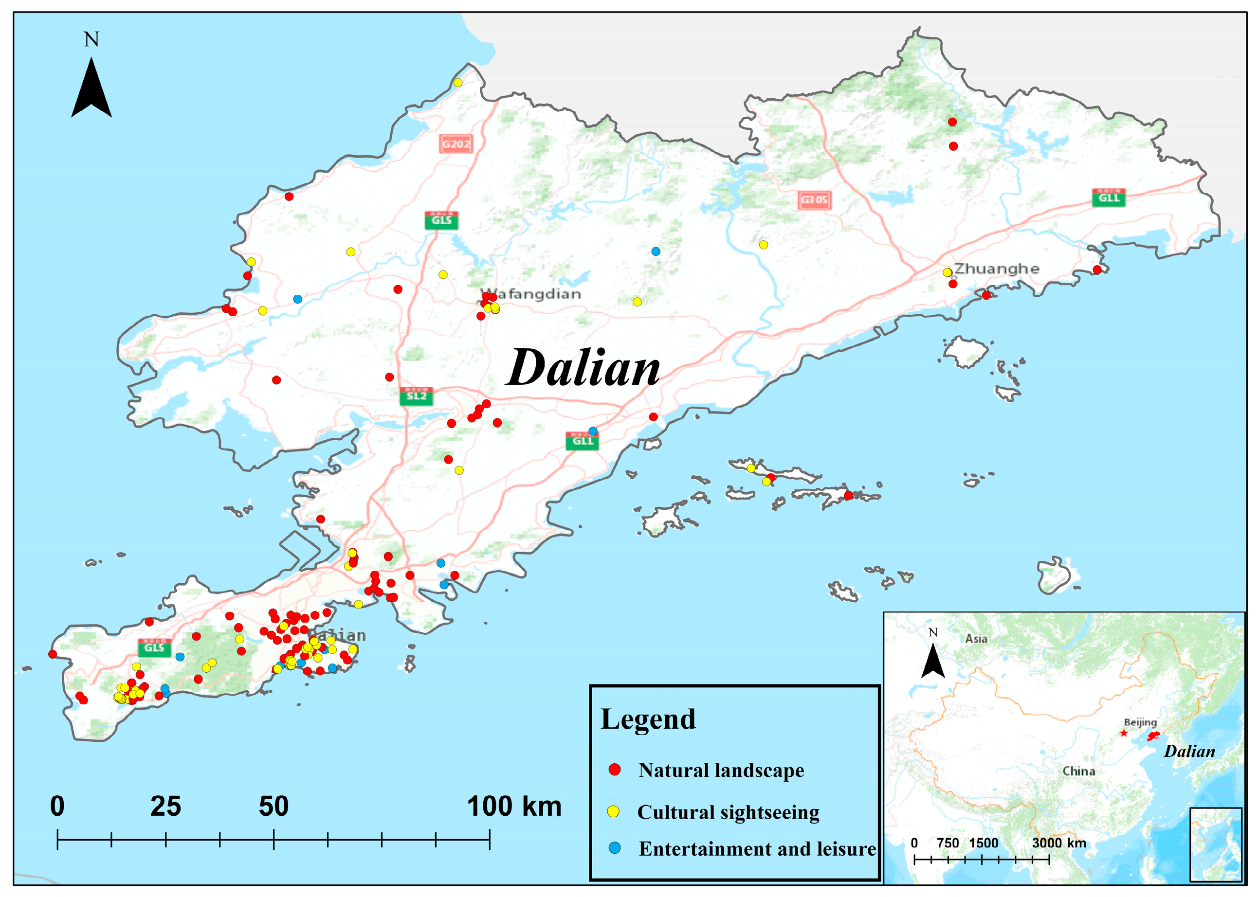
4.1. Study Area and Data

Dalian, located at the southern end of the Liaodong Peninsula, is one of China’s most popular coastal tourist supercities, with more than seven million permanent residents. It covers an area of 12,574 square kilometers and has a long coastline, stretching for thousands of kilometers, creating numerous sea-viewing spots. Dalian has witnessed most of China’s modern history and has various historical attractions. Figure 5 depicts the distribution of 151 major tourism attractions in Dalian, most of which are concentrated in urban areas.
Anonymous mobile tracking data consisting of user records and base station data are used as the data source. As shown in Table 1, a user record contains the encrypted user ID, base station ID (including LAC and CI), and timestamp. The anonymous mobile tracking data from 1 October 2020 to 3 October 2020 is used to derive crowd dynamics indices, whereas the data from 4 October 2020 is used to calculate the real-time hourly-updated crowd flow indicators to determine whether a dynamic adjustment is required during the tour. In addition, the basic attribute information (category and grade) and geographic information (geographical boundary coordinate) of the 151 attractions are obtained from online resources, including Baidu Map API (https://lbsyun.baidu.com, accessed on 17 October 2021) and Mafengwo (https://www.mafengwo.cn, accessed on 17 October 2021).

4.2. Derived Crowd Dynamics from Detected Tourism Activity Chains

In order to assess the accuracy of the rules for the tourist filtering strategy, the results of the number of tourist visits identified by the strategy were compared with official public data for the same period. The number of visitor visits for all attractions in Dalian and the Dalian Forest Zoo during the November holiday in 2020 was approximately 2,952,500 and 130,000, respectively. According to the contemporaneous results of the filtering strategy, the number of tourist visits to Dalian was 3,184,049, while Dalian Forest Zoo was 123,305, with relative errors of 7.84% and −5.15%, respectively. The results show that the accuracy of our filtering strategy is sufficiently guaranteed for macro tourism activity studies on an urban scale.
Approximately 0.89 million tourists are identified from 1 October to 3 October. Figure 6a depicts an example of a tourist’s two-day tourism activity chain. Figure 6b visualizes the crowd interaction network of attractions, where the nodes’ size represents the nodes’ degree of centrality; the thicker and denser the edges between nodes, the stronger the interaction between attractions. Notably, the significant tendency for the average degree and the average weighted degree suggests that the network interaction strength is generally weak in the morning and evening. Furthermore, according to its time differences, it can effectively confirm that it is necessary to take time factor into account when calculating attractions’ status. Figure 6c reflects the temporal variation of crowd flow indicators of the six example attractions in three days. Most attractions exhibit an upward-then-downward trend, with some experiencing a slight decline during midday. Figure 6d shows the crowd structure similarity S C S I in five different time windows, with horizontal and vertical coordinates representing the attraction’s IDs and the color in each pixel cell representing the S C S I between two attractions.

4.3. Algorithm Parameters

Several parameters affect the performance of INSGA-II, including operational population size ( P ), archival population size ( P A ), crossover probability ( P c ), mutation probability ( P m ), and maximum number of iterations ( G ). In this paper, the value of G is empirically set to 2000; P A is a multiple of P set to ten times of P . Eight sets of controlled trial experiments are designed to determine the appropriate values for the remaining parameters, including P , P c , and P m . In Table 2, E1, E2, E3, and E4 are the experiments designed for the parameter P , E2, E5, and E6 for parameter P c , and E2, E7, and E8 for parameter P m . Ten independent experiments are conducted for each set of parameters using the same dataset from Dalian.
The algorithm’s performance can be compared in terms of efficiency and effectiveness. Efficiency can be measured by the number of iterations and CPU time. For effectiveness, the algorithm can be evaluated using the hypervolume metric ( H V ), which can meassure convergence, distribution, and diversity of a solution set [62]. A larger value of HV indicates better performance.
H V X , P = x X X v ( x , P )
The comparison results of controlled trial experiments are shown in Figure 7. As P increases, the average number of iterations decreases. However, the average CPU time consumed for iterative convergence increases, which indicates that the increase in population size could significantly increase the computation time per generation. The mean HV value of E2 ( P = 50) is significantly larger than that of E1 ( P = 30) and E3 ( P = 70) and slightly lower than that of E4 ( P = 100). Considering the cost of calculation, it is more reasonable to set P to 50. For P c , E2 ( P c = 0.7) performs better than E5 ( P c = 0.5) for all three evaluations. Although E2 ( P c = 0.7) has a larger average number of convergent generations than E6 ( P c = 0.9), E2 ( P c = 0.7), it can reach convergence faster than E6 ( P c = 0.9). For P m , E2 ( P m = 0.2) is significantly more advantageous than E7 ( P m = 0.1) and E8 ( P m = 0.3). Therefore, considering the efficiency and effectiveness simultaneously, we set the parameters of our approach to the values listed in Table 3.

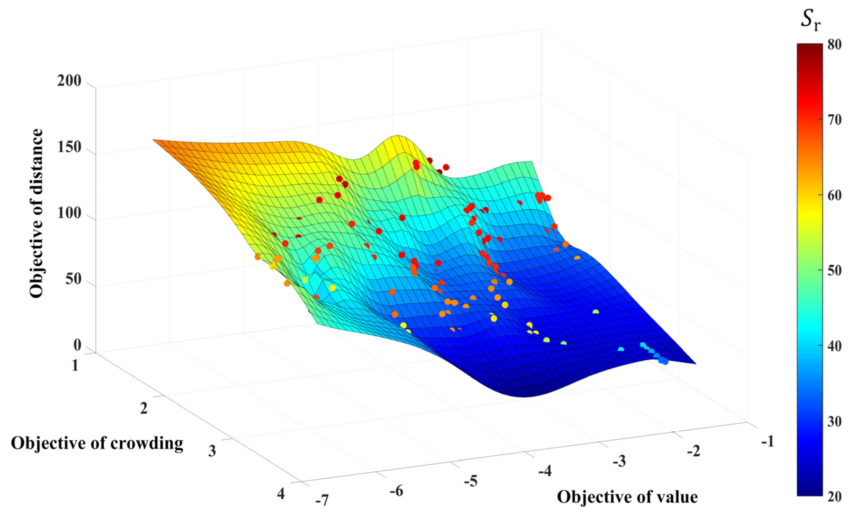
4.4. Optimization Results

In this part, a tourist is provided with the optimal scheme of routes, including the initial and adjusted routes, as an example of the optimization results. The tourist’s preference weights [ α n , α c , α e ] are [0.25, 0.5, 0.25]. The objective importance weights [ w C , w V , w D ] are [0.5, 0.3, 0.2]. The time budget is 8:00–18:30. The departure and final arrival locations are (121.62E, 38.90N) and (121.33E, 38.83N), respectively.

4.4.1. Initial Route Solutions

The algorithm is executed using the parameters listed in Table 3. Each run yields a set of non-dominated solutions. The initial stage was executed 20 times independently to avoid random errors and one-time occasionality. We extracted one of the 20 independent experiments and plotted the non-dominated solutions after the convergence in the three-dimensional space composed of three objectives, shown in Figure 8. These non-dominated solutions can be fitted into a three-dimensional surface and distributed evenly on the three targets, demonstrating that our method can obtain a well-distributed Pareto front.
The final non-dominated solutions are obtained by reevaluating the 20 sets of non-dominated solutions based on the dominance relationship. Each of the final non-dominant solutions can meet the needs of tourists with extensive objective values and has its emphasis on the three objectives. In this paper, a satisfaction evaluation function is developed to select a reference solution from the final non-dominated solutions that best satisfies the importance of different objectives for the tourist. With the tourist’s objective-importance weights for three objectives determined, the satisfaction of route r is calculated as follows:
S r = 100 × 1 w C f C , r f C , m i n f C , m a x f C , m i n + w V f V , r f V , m i n f V , m a x f V , m i n + w D f D , r f D , m i n f D , m a x f D , m i n
where f C , r , f V , r , f D , r denote the objective function values of route r . A larger value of S r indicates that the route is better considering the three objectives simultaneously according to the tourist’s needs.
Figure 9 depicts routes with three, four, and five spots of the selected reference solutions, with the red areas representing the scope of the to-visit attractions and the line charts representing the crowding flow indicator ( F ¯ i ) of the attractions involved in the routes. In the three routes, there is one 5A attraction (#92 Tiger Beach Ocean Park) and two 4A attractions (#12 Hengshan Temple and #67 Dalian Forest Zoo), which indicates that attractions with higher grades are more likely to be selected due to their high value. The remaining five attractions are not highly rated but are well located (close to highly rated attractions), have a high status in the attraction network, or fall within the tourist’s preferred category (cultural sightseeing category). For example, #27 Yanwo Mountain is 1.5 km away from the 5A-rated attraction #92 Tiger Beach Ocean Park and 3.4 km away from the 4A-rated attraction #67 Dalian Forest Zoo; and #107 Zhengjue Lecture Temple and #142 Jade Buddha Temple are cultural sightseeing attractions. Moreover, in the line charts of Figure 9, by correlating the visiting schedule and peak crowding period of each attraction, it can be concluded that the initial routes avoid the historical crowding peak in most cases.

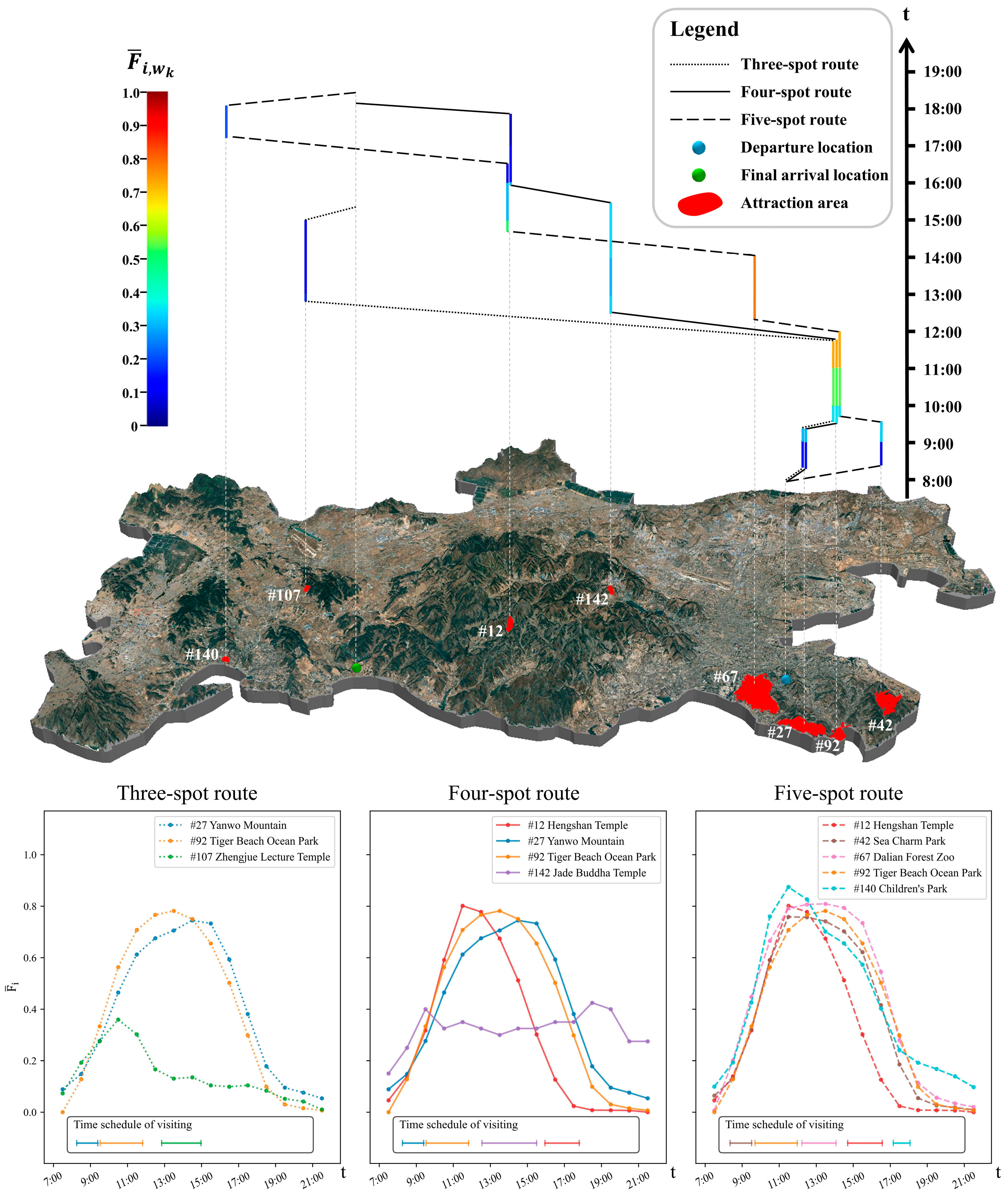
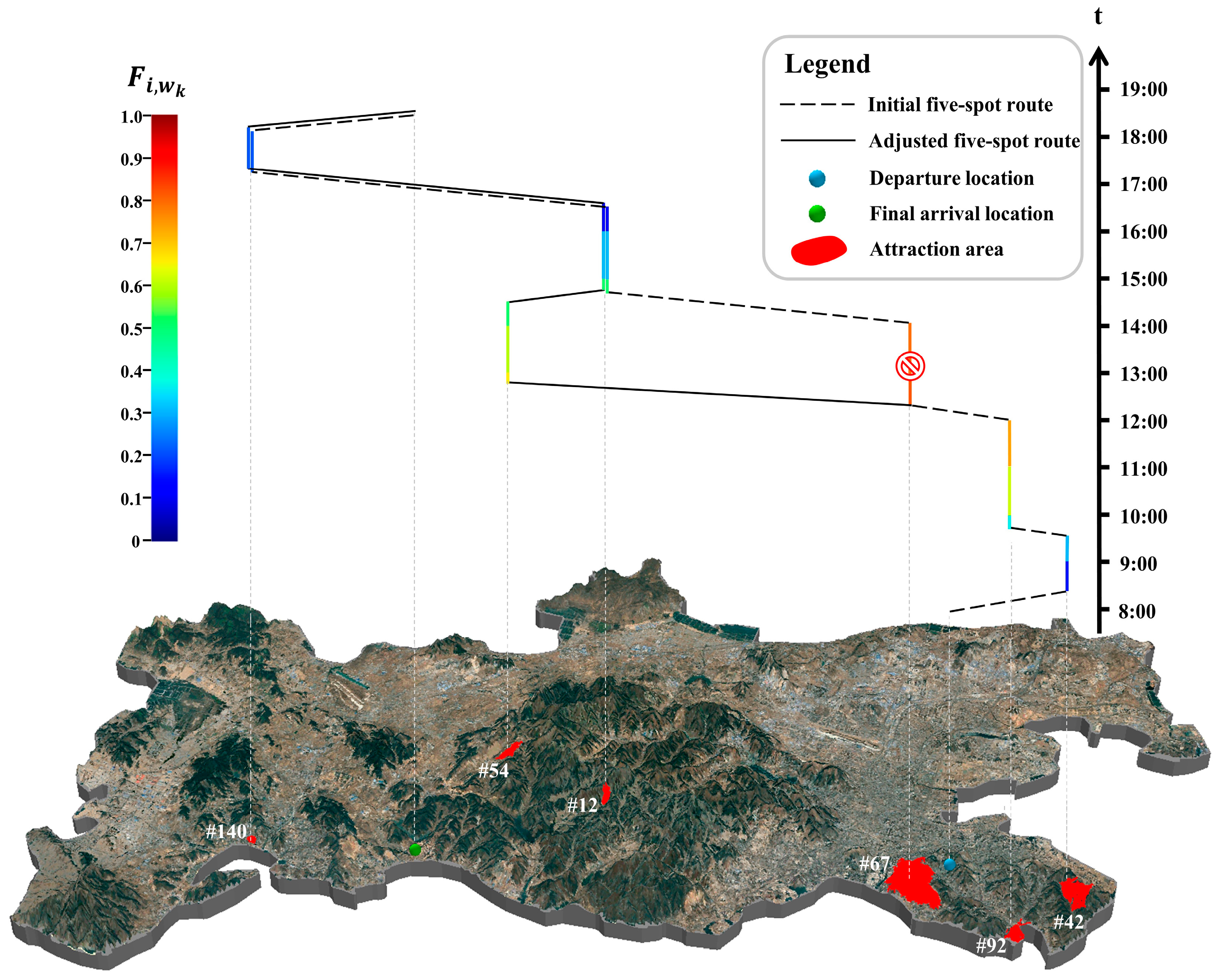
4.4.2. Adjusted Route Solutions

Adopting the strategy of the dynamic adjustment, the three initial routes are adjusted based on the real-time crowding flow indicator ( F i ) updated hourly on 4 October. In the adjustment stage, scale factor φ of the crowd threshold are set to be 0.8. According to the ratio of the longest distance to the average distance of the past tourist trips, the distance scale factor λ d is set to be 1.4. Among them, the five-spot route is adjusted due to the sudden increase in crowds, shown in Figure 10. One point to note is that although the route adjustment can reduce the crowding in the actual trip, it will unavoidably affect other objective values, and we attempt to minimize the three objectives.
In the adjusted route, #67 Dalian Forest Zoo is replaced by #54 Yinggeshi Botanical Garden. If the route is executed as the planned initial route, the value of the real-time crowding objective function would be 2.137, while after the adjustment, the value is 1.667, with a decrease of 21.99%, which indicates that the dynamic adjustment strategy can successfully provide alternatives to avoid sudden increases in crowds. Hence, the value objective function obtains a 28.01% increase after adjustment, from −8.303 to −5.977, due to the loss of the over-crowded 4A attraction #67 Dalian Forest Zoo, and the total distance increased by 17.769 km. This is the result of considering all three objectives simultaneously, which reduces the crowding at the expense of increases in the other objectives. Overall, dynamic route adjustment can be an excellent solution to sudden increases in crowds, providing tourists with a less-crowded route during the actual tour while minimizing the impact on other objectives.

5. Discussion

In this section, we compare the INSGA-II with other algorithms in terms of performance and solutions and evaluate the effectiveness of the dynamic adjustment by comparing the route solutions of the initial route and the dynamic adjustment stage. Considering the variations in individual preferences, constraints, and requirements in the practical applications, 20 tourist cases are designed in Table 4 according to the behavioral characteristics from mobile tracking data, in terms of category preference weights, objective importance weights, time budget, departure location, and final arrival location. The non-dominated sorting genetic algorithm II (NSGA-II), the multi-objective particle swarm optimization (MOPSO), the multi-objective ant colony optimization (MOACO), which are classical and widely used in solving the multi-objective TTDP [35], are used as baselines to compare with our INSGA-II. In addition to the above multi-objective optimization algorithms, the weighted sum method (WSM), one of the classical exact methods for multi-objective problems [63], is also involved in the comparison. To reduce random errors, each tourist’s experiment is conducted independently 20 times using each method.

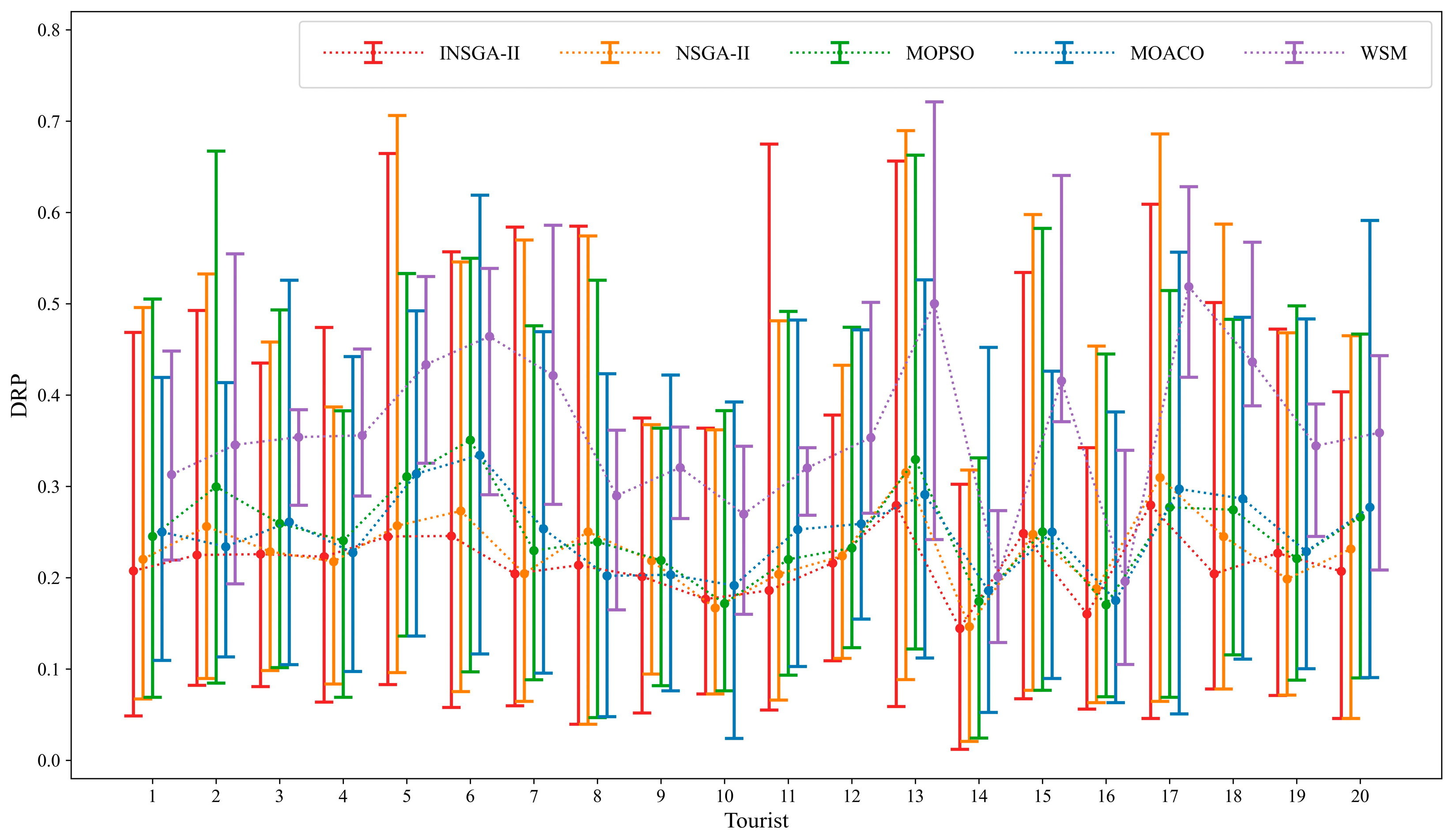
5.1. Performance Comparison

This section is dedicated to comparing the performance of various algorithms. The HV can be utilized to estimate the performance of the multi-objective optimization algorithms, which can be obtained according to Equation (23). As WSM is not a multi-objective optimization algorithm, it is not involved in this section.
As shown in Figure 11, our INSGA-II has larger average HVs than all the baseline methods for all tourists and has higher upper and lower bounds of HV in most cases, indicating that the non-dominated solutions obtained from INSGA-II have better convergence and distribution than the baseline methods. Moreover, INSGA-II has a narrow range of HVs across multiple independent experiments, demonstrating that INSGA-II is more robust. Generally, evolutionary algorithms (INSGA-II and NSGA-II) perform better than swarm intelligence-based algorithms (MOPSO and MOACO) in solving the proposed problem in this paper. All methods perform poorly in designing routes for tourist #4, #9, #10, and #17 with a tight time budget of no more than 9.5 h. Surprisingly, under such an extreme time budget, the INSGA-II performs significantly better than the baseline methods.

5.2. Solution Comparison

This section focuses on the solutions obtained from different methods by comparing the three objective function values of the final non-dominated solutions. As previously stated, for each tourist and method, the final non-dominated solutions are obtained according to the dominance relation of all non-dominated solutions from 20 independent experiments. Figure 12 depicts the final non-dominated solutions of five methods in the three-dimensional space of objectives. Obviously, compared with the baseline methods, our INSGA-II obtains more feasible non-dominated solutions, and the solutions from INSGA-II are closer to the minimum value of each objective, demonstrating that the INSGA-II algorithm can obtain more optimal solutions and a better Pareto front for the proposed multi-objective problem.
To quantitatively evaluate the final non-dominant solutions from different methods for all tourists, the distance to reference point (DRP) is calculated in Equation (25), denoted as the Euclidean distance between a final non-dominated solution (representing a feasible route) and the reference point ( O ). The three coordinate axes values of O are the minimum of the three objectives in the tourist’s final non-dominated solutions. Lower D P R indicates that the solution is more aligned to minimize the three objectives.
D R P r = o b j C , V , D N o r f o b j , r N o r f o b j , r e f 2
In Figure 13, for each tourist, with the D P R of all final non-dominated solutions from each algorithm calculated, the upper boundary, lower boundary, and middle point of the vertical bar indicates the maximum, minimum, and average D P R of these final non-dominated solutions, respectively. In Table 5, further information is extracted from Figure 13. Compared with baseline methods, the INSGA-II significantly obtains the lowest average D P R (70%) and the minimum D P R (95%) for most tourists. Therefore, the INSGA-II outperforms baseline methods in terms of optimality of solutions and can obtain the optimal solution in most cases.

5.3. Dynamic Adjustment Evaluation

This section focuses on evaluating the results of the dynamic adjustment stage by measuring the variations in the value of objectives, with the initial and dynamic adjustment stages implemented with INSGA-II. For each tourist, three kinds of initial reference solutions (three-spot, four-spot, and five-spot routes) are selected from the final non-dominated solutions of initial routes, according to the tourist’s needs (in Equation (24)). The initial reference solutions are used to access the dynamic adjustment stage proposed, which avoids overcrowded attractions by providing alternative attractions. Among these initial routes (including 20 three-spot routes, 20 four-spot routes, and 18 five-spot routes), the proposed method provides dynamic route adjustments for 8, 10, and 9 of them, respectively. The effect of the adjustment is measured by the relative change rate ( R C R ), which is calculated as follows:
R C R = m a d j u s t e d m i n i t i a l m i n i t i a l × 100 %
where m i n i t i a l and m a d j u s t e d denote different metrics of the initial and adjusted reference routes, which include the real-time crowding objective, value objective, distance objective, and total time spent.
The adjustment strategy aims to avoid the sudden increase in crowding while minimizing the three objectives; thus, the reduction of the objective values (reflected with negative R C R ) is expected. Figure 14 shows the R C R of route adjustment for all tourists. It can be seen that the adjustment achieves avoiding the sudden crowding increase and reduces the objective of real-time crowding (calculated with the real-time crowd flow indicators on 4 October) at the price of the increase in other objectives. Considering the crowd-avoiding goal in this paper, if this price is within the tolerable range, the goal of dynamic adjustment of the route is achieved.
In Table 6, further statistical results are analyzed with Figure 14. After the adjustment, 85.19% of the adjusted routes have a reduction in the real-time crowding, while 85.19% of them increase in the value objective, which indicates that the adjustment is implemented at the expense of the value objective in most cases. Surprisingly, the distance and total time spent decreased in most cases. In terms of R C R , the dynamic adjustment results in an average reduction of 7% in the crowding, with an average reduction of 7.95% and 6.74% in the distance and total time and an average increase of 10.87% in the value objective. Therefore, it can be concluded that the obtained value is mainly affected by the dynamic adjustments. Overall, the route adjustment in this paper achieves the purpose of avoiding crowds and providing real-time guidance and adjustment at an acceptable price.

6. Conclusions

Compared to the general TTDP, our proposed multi-objective model with a two-stage route strategy for solving the TTDP-CD aligns more with the needs of dynamic tour routes with a high-value tourism experience. This paper derives crowd dynamics information from 0.89 million historical tourism activity chains, including crowd flow, crowd interaction, and crowd structure of attractions. Crowd dynamics are used in a two-stage tour route design model with the strategy of “global optimization first and local update later.” In addition, the extended INSGA-II is employed to overcome the conflict of multiple objectives and search for the appropriate routes among multiple attractions.
This study performs various experiments to assess and validate the proposed methods and strategies. Three kinds of initial tour routes (three-spot, four-spot, and five spot routes) are designed for 20 tourists, and 27 of the 58 initial routes are dynamically adjusted due to sudden crowd increases, with the results showing that the dynamic adjustment reduces the real-time crowding by an average of 7%. Compared with baseline optimization algorithms, our INSGA-II is superior in algorithm performance, reflected by 100% frequency of the highest average hypervolume metric. The solution comparison indicates that our INSGA-II outperforms other baseline methods reflected with the 95% frequency of the optimal route solution.
We believe that our proposed TTDP-CD can provide a promising direction and reference for applying crowd dynamics to the tourism industry. The proposed approach to solving this problem could improve tourism service and management; for example, it could provide tourists with personalized tour routes with a sense of high-value experience and reduce congestion and crowd gathering in scenic spots for tourism management. The application of our approach can promote the tourism experience by reducing time or money wasted, balancing the activities between attractions, and encouraging the creation of online value-added tourism services.
There are several potential directions worthy of exploration in the future. Most tourists tend to travel in a group, making it essential for TTDPs to consider the preferences and constraints of all group members. It is feasible to split heterogeneous team groups for a while so that each homogeneous subgroup can pursue their interests separately before merging teams while considering the crow dynamics of these attractions. In addition, real-life users deserve more attention. One the one hand, future studies should take into consideration the factor of tourist crowding cognition and attraction affordability through research on real-life users while evaluating the crowding situation; on the other hand, empirical evaluation by real-life users can be extended to expand the application of TTDP study in evaluating the appropriateness of routes. The integration of multiple sources of data, such as RFID, Bluetooth base stations, and local questionnaires can further improve the expand the application feasibility of TTDP study.

Author Contributions

Conceptualization, Y.H. and Z.F.; methodology, Y.H.; software, Y.H., X.Z. and H.Z.; validation, Y.H., X.Z. and H.Z.; formal analysis, Y.H.; investigation, Z.F. and Y.H.; resources, Z.F.; data curation, Y.H. and H.Z.; writing—original draft preparation, Y.H.; writing—review and editing, Z.F. and L.W.; visualization, Y.H.; supervision, Z.F.; project administration, Z.F.; funding acquisition, Z.F. All authors have read and agreed to the published version of the manuscript.

Funding

This research was funded by the National Natural Science Foundation of China, grant number 41771473.

Institutional Review Board Statement

Not applicable.

Informed Consent Statement

Not applicable.

Data Availability Statement

Not applicable.

Conflicts of Interest

The authors declare no conflict of interest.

Appendix A

Table A1. Dividing point of interval bins for different behavioral indicators of tourists.
IndexDividing Point
Duration of stay[30.38, 40.81, 50.13, 59.44, 70.68, 84.68, 102.95, 129.73, 180.03]
Expense per day[0, 26, 98]
Number of attractions per day[1, 1.5, 2, 3]
Travel days[1, 2, 3]
Activity entropy[0, 0.43, 0.51, 0.65, 0.7707, 0.89, 0.98, 1.03]
Radius of gyration[53.82, 163.11, 284.95, 511.80, 940.39, 1671.35, 2934.14, 4356.37, 9996.55]

Appendix B

Table A2. Personalized parameters of 20 tourists.
IDCategory Preference WeightsObjective Importance WeightsTime BudgetDeparture LocationFinal Arrival Location
1[0.3, 0.2, 0.5][0.4, 0.3, 0.3]9:00–22:00[121.60, 38.91][121.60, 38.91]
2[0.25, 0.5, 0.25][0.5, 0.3, 0.2]8:00–18:30121.62, 38.90][121.33, 38.83]
3[0.7, 0.1, 0.2][0.333, 0.333, 0.333]8:30–22:00[121.18, 38.82][121.18, 38.82]
4[0.65, 0.2, 0.15][0.3, 0.3, 0.4]9:30–19:00[121.18, 38.82][121.45, 38.87]
5[0.3, 0.5, 0.2][0.4, 0.4, 0.2]8:00–22:00[121.64, 38.93][121.64, 38.93]
6[0.15, 0.6, 0.25][0.2, 0.5, 0.3]7:30–21:00[121.56, 38.89][121.56, 38.89]
7[0.3, 0.4, 0.4][0.333, 0.333, 0.333]10:00–21:30[121.69, 38.89][121.62, 38.91]
8[0.4, 0.1, 0.5][0.333, 0.333, 0.333]8:00–19:00[121.65, 38.93][121.65, 38.93]
9[0.65, 0.25, 0.1][0.4, 0.3, 0.3]10:00–19:00[121.29, 38.82][121.29, 38.82]
10[0.2, 0.2, 0.6][0.333, 0.333, 0.333]9:30–18:00[121.56, 38.89][121.54, 38.87]
11[0.35, 0.15, 0.5][0.3, 0.3, 0.4]8:00–22:00[121.62, 38.92][121.29, 38.82]
12[0.5, 0.3, 0.2][0.333, 0.333, 0.333]7:30–21:00[121.54, 38.87][121.69, 38.89]
13[0.1, 0.65, 0.25][0.4, 0.4, 0.2]10:00–22:00[121.63, 38.94][121.56, 38.94]
14[0.8, 0.1, 0.1][0.4, 0.3, 0.3]9:00–20:00[121.64, 38.93][121.66, 38.87]
15[0.55, 0.2, 0.25][0.5, 0.3, 0.2]9:30–21:00[121.81, 39.05][121.81, 39.05]
16[0.25, 0.1, 0.65][0.4, 0.3, 0.3]8:00–18:00[121.62, 38.91][121.56, 38.89]
17[0.1, 0.75, 0.15][0.4, 0.4, 0.2]8:00–17:30[121.81, 39.05][121.81, 39.05]
18[0.35, 0.35, 0.3][0.333, 0.333, 0.333]8:00–22:00[121.65, 38.93][121.62, 38.92]
19[0.4, 0.4, 0.2][0.3, 0.3, 0.4]9:30–19:00[121.64, 38.93][121.64, 38.93]
20[0.25, 0.25, 0.5][0.333, 0.333, 0.333]9:00–22:00[121.59, 38.91][121.59, 38.91]

References

  1. Borràs, J.; Moreno, A.; Valls, A. Intelligent Tourism Recommender Systems: A Survey. Expert Syst. Appl. 2014, 41, 7370–7389. [Google Scholar] [CrossRef]
  2. Gavalas, D.; Konstantopoulos, C.; Mastakas, K.; Pantziou, G. Mobile Recommender Systems in Tourism. J. Netw. Comput. Appl. 2014, 39, 319–333. [Google Scholar] [CrossRef]
  3. Hamid, R.A.; Albahri, A.S.; Alwan, J.K.; Al-qaysi, Z.T.; Albahri, O.S.; Zaidan, A.A.; Alnoor, A.; Alamoodi, A.H.; Zaidan, B.B. How Smart Is E-Tourism? A Systematic Review of Smart Tourism Recommendation System Applying Data Management. Comput. Sci. Rev. 2021, 39, 100337. [Google Scholar] [CrossRef]
  4. Rodríguez, B.; Molina, J.; Pérez, F.; Caballero, R. Interactive Design of Personalised Tourism Routes. Tour. Manag. 2012, 33, 926–940. [Google Scholar] [CrossRef]
  5. Vansteenwegen, P.; Van Oudheusden, D. The Mobile Tourist Guide: An OR Opportunity. OR Insight 2007, 20, 21–27. [Google Scholar] [CrossRef]
  6. Liao, Z.; Zheng, W. Using a Heuristic Algorithm to Design a Personalized Day Tour Route in a Time-Dependent Stochastic Environment. Tour. Manag. 2018, 68, 284–300. [Google Scholar] [CrossRef]
  7. Zheng, W.; Ji, H.; Lin, C.; Wang, W.; Yu, B. Using a Heuristic Approach to Design Personalized Urban Tourism Itineraries with Hotel Selection. Tour. Manag. 2020, 76, 103956. [Google Scholar] [CrossRef]
  8. Liao, Z.; Zhang, X.; Zhang, Q.; Zheng, W.; Li, W. Rough Approximation-Based Approach for Designing a Personalized Tour Route under a Fuzzy Environment. Inf. Sci. 2021, 575, 338–354. [Google Scholar] [CrossRef]
  9. De Falco, I.; Scafuri, U.; Tarantino, E. A Multiobjective Evolutionary Algorithm for Personalized Tours in Street Networks. In Applications of Evolutionary Computation; Mora, A.M., Squillero, G., Eds.; Springer International Publishing: Cham, Switzerland, 2015; Volume 9028, pp. 115–127. ISBN 978-3-319-16548-6. [Google Scholar]
  10. Zheng, W.; Liao, Z.; Lin, Z. Navigating through the Complex Transport System: A Heuristic Approach for City Tourism Recommendation. Tour. Manag. 2020, 81, 104162. [Google Scholar] [CrossRef]
  11. Lim, K.H.; Chan, J.; Karunasekera, S.; Leckie, C. Tour Recommendation and Trip Planning Using Location-Based Social Media: A Survey. Knowl. Inf. Syst. 2019, 60, 1247–1275. [Google Scholar] [CrossRef]
  12. Lamsfus, C.; Martín, D.; Alzua-Sorzabal, A.; Torres-Manzanera, E. Smart Tourism Destinations: An Extended Conception of Smart Cities Focusing on Human Mobility. In Information and Communication Technologies in Tourism 2015; Tussyadiah, I., Inversini, A., Eds.; Springer International Publishing: Cham, Switzerland, 2015; pp. 363–375. ISBN 978-3-319-14342-2. [Google Scholar]
  13. Moyle, B.; Croy, G. Crowding and Visitor Satisfaction During the Off-season: Port Campbell National Park. Ann. Leis. Res. 2007, 10, 518–531. [Google Scholar] [CrossRef]
  14. Zehrer, A.; Raich, F. The Impact of Perceived Crowding on Customer Satisfaction. J. Hosp. Tour. Manag. 2016, 29, 88–98. [Google Scholar] [CrossRef]
  15. Liu, J.; Wood, K.L.; Lim, K.H. Strategic and Crowd-Aware Itinerary Recommendation. In Machine Learning and Knowledge Discovery in Databases: Applied Data Science Track; Dong, Y., Mladenić, D., Saunders, C., Eds.; Springer International Publishing: Cham, Switzerland, 2021; Volume 12460, pp. 69–85. ISBN 978-3-030-67666-7. [Google Scholar]
  16. Yu, F.-C.; Lee, P.-C.; Ku, P.-H.; Wang, S.-S. A Theme Park Tourist Service System with a Personalized Recommendation Strategy. Appl. Sci. 2018, 8, 1745. [Google Scholar] [CrossRef] [Green Version]
  17. Park, S.; Xu, Y.; Jiang, L.; Chen, Z.; Huang, S. Spatial Structures of Tourism Destinations: A Trajectory Data Mining Approach Leveraging Mobile Big Data. Ann. Tour. Res. 2020, 84, 102973. [Google Scholar] [CrossRef]
  18. Zheng, W.; Li, M.; Lin, Z.; Zhang, Y. Leveraging Tourist Trajectory Data for Effective Destination Planning and Management: A New Heuristic Approach. Tour. Manag. 2022, 89, 104437. [Google Scholar] [CrossRef]
  19. Augstein, M.; Herder, E.; Wörndl, W. (Eds.) Tourist Trip Recommendations—Foundations, State of the Art, and Challenges. In Personalized Human-Computer Interaction; De Gruyter Oldenbourg: Berlin, Germany, 2019; pp. 159–182. ISBN 978-3-11-055248-5. [Google Scholar]
  20. Hyde, K.F.; Lawson, R. The Nature of Independent Travel. J. Travel Res. 2003, 42, 13–23. [Google Scholar] [CrossRef]
  21. Kotiloglu, S.; Lappas, T.; Pelechrinis, K.; Repoussis, P.P. Personalized Multi-Period Tour Recommendations. Tour. Manag. 2017, 62, 76–88. [Google Scholar] [CrossRef] [Green Version]
  22. Gavalas, D.; Konstantopoulos, C.; Mastakas, K.; Pantziou, G. A Survey on Algorithmic Approaches for Solving Tourist Trip Design Problems. J. Heuristics 2014, 20, 291–328. [Google Scholar] [CrossRef]
  23. Tsiligirides, T. Heuristic Methods Applied to Orienteering. J. Oper. Res. Soc. 1984, 35, 797. [Google Scholar] [CrossRef]
  24. Kantor, M.G.; Rosenwein, M.B. The Orienteering Problem with Time Windows. J. Oper. Res. Soc. 1992, 43, 629–635. [Google Scholar] [CrossRef]
  25. Fomin, F.V.; Lingas, A. Approximation Algorithms for Time-Dependent Orienteering. Inf. Process. Lett. 2002, 83, 57–62. [Google Scholar] [CrossRef]
  26. Archetti, C.; Hertz, A.; Speranza, M.G. Metaheuristics for the Team Orienteering Problem. J. Heuristics 2007, 13, 49–76. [Google Scholar] [CrossRef]
  27. Tlili, T.; Krichen, S. A Simulated Annealing-Based Recommender System for Solving the Tourist Trip Design Problem. Expert Syst. Appl. 2021, 186, 115723. [Google Scholar] [CrossRef]
  28. Ko, T.; Qureshi, A.G.; Schmöcker, J.-D.; Fujii, S. Tourist Trip Design Problem Considering Fatigue. J. East. Asia Soc. Transp. Stud. 2019, 13, 1233–1248. [Google Scholar] [CrossRef]
  29. Trachanatzi, D.; Rigakis, M.; Marinaki, M.; Marinakis, Y. An Interactive Preference-Guided Firefly Algorithm for Personalized Tourist Itineraries. Expert Syst. Appl. 2020, 159, 113563. [Google Scholar] [CrossRef]
  30. Divsalar, G.; Divsalar, A.; Jabbarzadeh, A.; Sahebi, H. An Optimization Approach for Green Tourist Trip Design. Soft Comput. 2022, 26, 4303–4332. [Google Scholar] [CrossRef]
  31. Talbi, E.-G. Metaheuristics: From Design to Implementation; John Wiley & Sons: Hoboken, NJ, USA, 2009; ISBN 978-0-470-27858-1. [Google Scholar]
  32. Verbeeck, C.; Vansteenwegen, P.; Aghezzaf, E.-H. An Extension of the Arc Orienteering Problem and Its Application to Cycle Trip Planning. Transp. Res. Part E Logist. Transp. Rev. 2014, 68, 64–78. [Google Scholar] [CrossRef]
  33. Kwon, W.Y.; Kim, M.; Suh, I.H. Probabilistic Tourist Trip-Planning with Time-Dependent Human and Environmental Factors. In Proceedings of the 2016 International Conference on Big Data and Smart Computing (BigComp), Hong Kong, China, 18–20 January 2016; pp. 505–508.
  34. Wang, X.; Leckie, C.; Chan, J.; Lim, K.H.; Vaithianathan, T. Improving Personalized Trip Recommendation by Avoiding Crowds. In Proceedings of the 25th ACM International on Conference on Information and Knowledge Management, Indianapolis, IN, USA, 24–28 October 2016; pp. 25–34. [Google Scholar]
  35. Ruiz-Meza, J.; Montoya-Torres, J.R. A Systematic Literature Review for the Tourist Trip Design Problem: Extensions, Solution Techniques and Future Research Lines. Oper. Res. Perspect. 2022, 9, 100228. [Google Scholar] [CrossRef]
  36. Gavalas, D.; Kasapakis, V.; Konstantopoulos, C.; Pantziou, G.; Vathis, N.; Zaroliagis, C. The ECOMPASS Multimodal Tourist Tour Planner. Expert Syst. Appl. 2015, 42, 7303–7316. [Google Scholar] [CrossRef]
  37. Kurata, Y.; Hara, T. CT-Planner. In Information and Communication Technologies in Tourism 2014; Xiang, Z., Tussyadiah, I., Eds.; Springer International Publishing: Cham, Switzerland, 2013; pp. 73–86. ISBN 978-3-319-03972-5. [Google Scholar]
  38. Barbosa, H.; Barthelemy, M.; Ghoshal, G.; James, C.R.; Lenormand, M.; Louail, T.; Menezes, R.; Ramasco, J.J.; Simini, F.; Tomasini, M. Human Mobility: Models and Applications. Phys. Rep. 2018, 734, 1–74. [Google Scholar] [CrossRef]
  39. Hernández, J.M.; Santana-Jiménez, Y.; González-Martel, C. Factors Influencing the Co-Occurrence of Visits to Attractions: The Case of Madrid, Spain. Tour. Manag. 2021, 83, 104236. [Google Scholar] [CrossRef]
  40. Mou, N.; Zheng, Y.; Makkonen, T.; Yang, T.; Tang, J.; Song, Y. Tourists’ Digital Footprint: The Spatial Patterns of Tourist Flows in Qingdao, China. Tour. Manag. 2020, 81, 104151. [Google Scholar] [CrossRef]
  41. Xu, Y.; Xue, J.; Park, S.; Yue, Y. Towards a Multidimensional View of Tourist Mobility Patterns in Cities: A Mobile Phone Data Perspective. Comput. Environ. Urban Syst. 2021, 86, 101593. [Google Scholar] [CrossRef]
  42. Popp, M. Positive and Negative Urban Tourist Crowding: Florence, Italy. Tour. Geogr. 2012, 14, 50–72. [Google Scholar] [CrossRef]
  43. Cheng, H.; Liu, Q.; Bi, J.-W. Perceived Crowding and Festival Experience: The Moderating Effect of Visitor-to-Visitor Interaction. Tour. Manag. Perspect. 2021, 40, 100888. [Google Scholar] [CrossRef]
  44. Jacobsen, J.K.S.; Iversen, N.M.; Hem, L.E. Hotspot Crowding and Over-Tourism: Antecedents of Destination Attractiveness. Ann. Tour. Res. 2019, 76, 53–66. [Google Scholar] [CrossRef]
  45. Kainthola, S.; Tiwari, P.; Chowdhary, N.R. Overtourism to Zero Tourism: Changing Tourists’ Perception of Crowding Post COVID-19. J. Spat. Organ. Dyn. 2021, 9, 115–137. [Google Scholar]
  46. Casanueva, C.; Gallego, Á.; García-Sánchez, M.-R. Social Network Analysis in Tourism. Curr. Issues Tour. 2016, 19, 1190–1209. [Google Scholar] [CrossRef]
  47. McPherson, M.; Smith-Lovin, L.; Cook, J.M. Birds of a Feather: Homophily in Social Networks. Annu. Rev. Sociol. 2001, 27, 415–444. [Google Scholar] [CrossRef] [Green Version]
  48. Tsai, C.-Y.; Chung, S.-H. A Personalized Route Recommendation Service for Theme Parks Using RFID Information and Tourist Behavior. Decis. Support Syst. 2012, 52, 514–527. [Google Scholar] [CrossRef]
  49. Li, Y.; Yang, L.; Shen, H.; Wu, Z. Modeling Intra-Destination Travel Behavior of Tourists through Spatio-Temporal Analysis. J. Destin. Mark. Manag. 2019, 11, 260–269. [Google Scholar] [CrossRef]
  50. Sun, Y.; Shao, Y.; Chan, E.H.W. Co-Visitation Network in Tourism-Driven Peri-Urban Area Based on Social Media Analytics: A Case Study in Shenzhen, China. Landsc. Urban Plan. 2020, 204, 103934. [Google Scholar] [CrossRef]
  51. Li, J.; Xu, L.; Tang, L.; Wang, S.; Li, L. Big Data in Tourism Research: A Literature Review. Tour. Manag. 2018, 68, 301–323. [Google Scholar] [CrossRef]
  52. Schmöcker, J.-D. Estimation of City Tourism Flows: Challenges, New Data and COVID. Transp. Rev. 2021, 41, 137–140. [Google Scholar] [CrossRef]
  53. Ye, B.H.; Ye, H.; Law, R. Systematic Review of Smart Tourism Research. Sustainability 2020, 12, 3401. [Google Scholar] [CrossRef] [Green Version]
  54. Gretzel, U.; Sigala, M.; Xiang, Z.; Koo, C. Smart Tourism: Foundations and Developments. Electron. Mark. 2015, 25, 179–188. [Google Scholar] [CrossRef] [Green Version]
  55. Qian, C.; Li, W.; Duan, Z.; Yang, D.; Ran, B. Using Mobile Phone Data to Determine Spatial Correlations between Tourism Facilities. J. Transp. Geogr. 2021, 92, 103018. [Google Scholar] [CrossRef]
  56. Raun, J.; Ahas, R.; Tiru, M. Measuring Tourism Destinations Using Mobile Tracking Data. Tour. Manag. 2016, 57, 202–212. [Google Scholar] [CrossRef]
  57. Pappalardo, L.; Vanhoof, M.; Gabrielli, L.; Smoreda, Z.; Pedreschi, D.; Giannotti, F. An Analytical Framework to Nowcast Well-Being Using Mobile Phone Data. Int. J. Data Sci. Anal. 2016, 2, 75–92. [Google Scholar] [CrossRef] [Green Version]
  58. González, M.C.; Hidalgo, C.A.; Barabási, A.-L. Understanding Individual Human Mobility Patterns. Nature 2008, 453, 779–782. [Google Scholar] [CrossRef]
  59. Castellani, M.; Pattitoni, P.; Vici, L. Pricing Visitors’ Preferences for Temporary Art Exhibitions. SSRN J. 2012, 21, 83–103. [Google Scholar] [CrossRef]
  60. Zheng, W.; Liao, Z.; Qin, J. Using a Four-Step Heuristic Algorithm to Design Personalized Day Tour Route within a Tourist Attraction. Tour. Manag. 2017, 62, 335–349. [Google Scholar] [CrossRef]
  61. Deb, K.; Pratap, A.; Agarwal, S.; Meyarivan, T. A Fast and Elitist Multiobjective Genetic Algorithm: NSGA-II. IEEE Trans. Evol. Computat. 2002, 6, 182–197. [Google Scholar] [CrossRef] [Green Version]
  62. Shang, K.; Ishibuchi, H.; He, L.; Pang, L.M. A Survey on the Hypervolume Indicator in Evolutionary Multiobjective Optimization. IEEE Trans. Evol. Computat. 2021, 25, 1–20. [Google Scholar] [CrossRef]
  63. Marler, R.T.; Arora, J.S. The Weighted Sum Method for Multi-Objective Optimization: New Insights. Struct. Multidisc. Optim. 2010, 41, 853–862. [Google Scholar] [CrossRef]
Figure 1. Information derivation and route recommendation strategies for TTDP-CD. The crowd flow, reflected by the time-varying crowd flow indicator F i , is used to assist tourists in avoiding peak hours. The crowd interaction between attractions reveals the status of each attraction in the interaction network, which is reflected by the degree of nodes D i , i n and D i , o u t and is used to determine the value of destinations. As the dynamic adjustment is activated, the attraction replacement scheme is determined by the similarity of the crowd structure S C S I .
Applsci 13 00596 g001
Figure 2. A user’s record of points and trajectory in the process of sightseeing. L 1 L 15 represent the location of recorded points from mobile tracking data. Points at attraction A ( L 2 L 6 ) record the first attraction stay in the user’s trajectory, while points at attraction B ( L 10 L 13 ) record the second one. These stays constitute the user’s stay sequences at attractions. Only after the user is identified as a tourist of attraction A and attraction B by the tourist filtering strategy can these detected stays be determined as tourism activities, which are used to construct tourism activity chains.
Applsci 13 00596 g002
Figure 3. Process of the two-stage route strategy.
Applsci 13 00596 g003
Figure 4. Representation of the chromosome and evolutionary operators: (a) container-index coding and decoding; (b) partial-mapped crossover operator; (c) mixed mutation operators.
Applsci 13 00596 g004
Figure 5. Distribution of major tourism attractions in Dalian.
Applsci 13 00596 g005
Figure 6. Derived results of crowd dynamics from tourism activity chains: (a) an example of tourism activity chain; (b) interaction network of attractions; (c) crowd flow indicator of attractions; (d) similarity of crowd structure of attractions.
Applsci 13 00596 g006
Figure 7. Algorithm evaluation results under different parameters. The three vertical columns are the controlled trial experiments on different kinds of parameters, including P , P c , and P m . The three horizontal rows demonstrate the indicators of the experiment results to evaluate the algorithm’s performance under different parameters, including average iteration times, average CPU time, and average HV.
Applsci 13 00596 g007
Figure 8. Non-dominated solutions of initial route solutions of one independent experiment. The three axes correspond to the three minimized objective function values. The satisfaction evaluation S r of each non-dominated solution (represented as a dot) can refer to the values on the color scale according to the dot’s color.
Applsci 13 00596 g008
Figure 9. Initial routes designed for the tourist and the historical crowd flow indicator ( F ¯ i ) of the involved attractions.
Applsci 13 00596 g009
Figure 10. Routes before and after the dynamic adjustment.
Applsci 13 00596 g010
Figure 11. The comparison of average, maximum, and minimum HV values for 20 different tourists (INSGA-II, NSGA-II, MOPSO, and MOACO).
Applsci 13 00596 g011
Figure 12. The final non-dominated solutions from different methods (an example of tourist #12).
Applsci 13 00596 g012
Figure 13. The comparison of average, maximum and minimum DRP value for 20 different tourists (INSGA-II, NSGA-II, MOPSO, MOACO, and WSM).
Applsci 13 00596 g013
Figure 14. The comparison of objective function values of routes before and after adjustment: (a) Three spot route; (b) four-spot route; (c) five-spot route.
Applsci 13 00596 g014
Table 1. Example of raw records of mobile tracking data.
User IDCILACTimestamp
0000****c2b8167822237761942020/10/1 11:49:56
0000****c2b816659608629872020/10/1 11:52:16
000b****497c16810685396592020/10/1 14:10:00
000b****497c167662264222452020/10/1 14:12:58
Table 2. Eight comparative experiments were performed to test the appropriate parameter.
Experiment P P c P m
E1300.70.2
E2500.70.2
E3700.70.2
E41000.70.2
E5500.50.2
E6500.90.2
E7500.70.1
E8500.70.3
Table 3. Parameters of the INSGA-II algorithm.
Parameters P P c P m P A G
Values500.70.25002000
Table 4. Personalized information of the 20 designed tourist cases.
IDCategory Preference WeightsObjective Importance WeightsTime BudgetDeparture LocationFinal Arrival Location
1[0.3, 0.2, 0.5][0.4, 0.3, 0.3]9:00–22:00[121.60, 38.91][121.60, 38.91]
2[0.25, 0.5, 0.25][0.5, 0.3, 0.2]8:00–18:30[121.62, 38.90][121.33, 38.83]
19[0.4, 0.4, 0.2][0.3, 0.3, 0.4]9:30–19:00[121.64, 38.93][121.64, 38.93]
20[0.25, 0.25, 0.5][0.333, 0.333, 0.333]9:00–22:00[121.59, 38.91][121.59, 38.91]
The complete version is in Table A2 in the Appendix B.
Table 5. The frequency of lowest average DRP and minimum DRP in 20 tourists by INSGA-II, NSGA-II, MOPSO, MOACO, WSM.
MethodFrequency of Lowest Average DRPFrequency of the Minimum DRP
INSGA-II14 (70%)19 (95%)
NSGA-II4 (20%)4 (20%)
MOPSO1 (5%)0 (0%)
MOACO1 (5%)1 (5%)
WSM0 (0%)0 (0%)
Table 6. The RCR of four metrics after the adjustment.
MetricsCount of Reduced CasesCount of Increased CasesAverage RCR
Real-time crowding23 (85.19%)4 (14.81%)−7.00%
Value objective4 (14.81%)23 (85.19%)10.87%
Distance objective20 (74.07%)7 (25.93%)−7.95%
Total time23 (85.19%)4 (14.81%)−6.74%
Disclaimer/Publisher’s Note: The statements, opinions and data contained in all publications are solely those of the individual author(s) and contributor(s) and not of MDPI and/or the editor(s). MDPI and/or the editor(s) disclaim responsibility for any injury to people or property resulting from any ideas, methods, instructions or products referred to in the content.

