Application of Microtremor Survey Technology in a Coal Mine Goaf

Abstract

Goafs are one of the main factors that endanger the safety of mining areas, leading to roadway collapse, land subsidence and other problems. Determining how to detect goafs accurately and efficiently is an important issue faced in engineering geophysical exploration research. Microtremor survey technology, used in geophysical exploration, has been developed in recent years. It has the advantages of low cost, flexible construction, low topographic impact and high efficiency. In this paper, microtremor survey technology was applied to the detection of a coal mine goaf. In the known goaf area of the Taiyuan Nanling Coal Mine, a linear observation array was arranged to conduct rolling acquisition, observe the microtremor signal records of the natural field and use the extended spatial autocorrelation method to extract the dispersion curve. Through the inversion of the extracted dispersion curve, the apparent shear wave velocity profile of the underground medium clearly showed the location of the goaf. It was roughly consistent with the goaf data obtained from the mine. The detection results reflect the advantages of micromotion exploration. The goaf of Coal Seam #2 and its affected area appear to be due to an obvious low-speed phenomenon. The boundary of the apparent shear wave velocity profile of micromotion detection was basically consistent with the boundary of the goaf, indicating that micromotion exploration technology has good technical advantages and application prospects in the detection of coal mine goafs. The rolling acquisition method of linear arrays can be used to ensure accurate detection, improve exploration efficiency and save on exploration costs.

1. Introduction

The geological structure of the goaf in the Nanling mining area is very complex, with developed fractures. After the mining of underground coal seams in this mining area, the goaf is one of the significant hidden dangers affecting the safety of the mining area. If the goaf collapses and fills with water, it will endanger the life and safety of the personnel in the mining area. Therefore, it is particularly important to determine the specific location of the goaf. At present, the electrical method, the magnetic method, the seismic method, geological radar, geological drilling and other methods are commonly used. Xue Guoqiang et al. (2013) used the transient electromagnetic method to detect the goaf water-filling area around a power transmission and transformation station in western Shanxi Province, and the results were in good agreement with the drilling data [1]. Qin Si et al. (2015) carried out combined ground well and seismic advance exploration in a coal mine in northern Shaanxi. The results showed that the exploration of abandoned roadways and goafs in front of coal seams had a positive effect [2]. Cai Guangtao et al. (2021) established a geological model and used geological drilling methods to evaluate the stability of a medium-length highway tunnel built above a multi-layer goaf [3]. Xu Xichang et al. (2009) used the high-density electrical method and geological radar to detect abandoned mines, and the results were confirmed by later excavation detection [4].

Micromotion exploration, also known as natural source surface wave exploration, has a long history. The extraction of surface waves from natural earthquakes can be traced back to the 1950s or even earlier. It is a relatively new method to extract surface waves from a microtremor and make them practically useful. Aki (1957) theoretically deduced for the first time the spatial autocorrelation method (SPAC). This method assumes that the microtremor conforms to a stationary random process in time and space. He used this method to obtain the dispersion curve of a Rayleigh wave from the microtremor signal [5]. Capon (1969) proposed the frequency wave number method (F-K), and used this method to extract the surface wave dispersion curve from the fretting signal [6]. For a long time after the above two methods were proposed, microtremor survey technology basically remained in the theoretical research stage, and was not applied to practical research. Okada (2003) improved the SPAC method, set different observation radii and applied the extended spatial autocorrelation method (ESPAC) to multiple observation arrays, which significantly improved data processing efficiency [7]. Due to the improvement of the SPAC method, the array layout became more flexible, which expanded microtremor exploration from theory to practical application. Ohori et al. (2002) used the ESPAC method to estimate shear wave velocity structure with a formation depth of 43 m, and the results were in good agreement with the P-S logging profile. When using an arbitrarily shaped array to determine the Rayleigh wave phase velocity, the ESPAC method is more accurate than the F-K method [8]. Feng Shaokong (2003) applied microtremor exploration technology to the field of civil engineering. He observed the microtremor data of the test site through a double concentric nested triangle array. The results showed that the subsurface shear wave velocity model obtained by microtremor exploration is generally consistent with the traditional P-S logging results [9]. Ye Tailan (2004) explored at a depth of 3000 m using the microtremor exploration method [10]. Xu Peifen et al. (2013) used microtremor detection technology to detect stratum stratification and hidden faults, achieving good results [11]. Tian Baoqing et al. (2017) took the geothermal resource area in southern Jiangsu as an example to analyze the effect of micromotion survey, as well as geological and technical factors such as observation radius and sampling frequency, by comparing the results of microtremor exploration and drilling. The applicability of the microtremor detection method was studied, and a good detection effect was obtained [12]. Huang Huicong et al. (2022) carried out microdynamics surveys at 53 sites in Taichung, Taiwan, China, and the results indicated that the thickness of the alluvium decreases from west to east, which is consistent with the geology of the Taichung area [13]. In recent years, microtremor exploration has achieved results in the field of goaf exploration; for instance, Ma Guosong (2022) applied the microtremor method to the exploration of a water-rich goaf for the first time. He carried out the high-density electrical method and micromotion detection in a known goaf area of Qingdao Metro Line 8, and obtained a micromotion shear wave apparent velocity profile that clearly showed the location of the goaf, which was consistent with the results of high-density electrical method inversion and borehole sampling [14]. A series of microtremor detection results has shown that the microtremor exploration is sensitive to the response of an underground abnormal high-velocity body and an abnormal low-velocity body, and can accurately locate the abnormal body.

This paper considered the goaf of the Nanling Coal Mine in Taiyuan City as the research object, verified the goaf of Coal Seam #2 and its area of influence through known data and processed and analyzed the collected fretting data after field experiments. The experimental results prove that the fretting method can effectively detect the goaf. The conventional method of microtremor exploration is to use triangle array for data acquisition. This experiment innovatively used the rolling acquisition method of linear array, which can also obtain better detection results, greatly improve exploration efficiency and save on exploration costs.

2. Principle of Microtremor Exploration

At any time, and anywhere on the earth’s surface, there is a weak vibration. This continuous weak vibration is called microtremor, which mainly comes from two aspects: first, it is caused by natural phenomena such as air pressure, wind speed, waves and tidal changes; second, it is caused by processes such as vehicle driving, machine operation and people’s daily production activities [11]. Microtremor is a kind of complex vibration without a specific source. The energy of these vibrations spreads into the distance in the form of waves, the main form of propagation being surface waves. Microtremor exploration is one of the geophysical exploration methods that use the observation system to record surface waves, extract the dispersion information contained therein and then infer the S-wave velocity structure of the underground medium. At present, there are two commonly used methods to extract the dispersion curve; one is the SPAC method, and the second is the F-K method. We used the SPAC method in this study.

2.1. SPAC

The SPAC method is based on two basic assumptions: (1) the microtremor accords with a stationary random process in time and space; and (2) the fundamental order surface wave is dominant among all kinds of waves included in the microtremor. The basic principle of the SPAC method is as follows.

The SPAC method is a data-processing method to obtain a microtremor signal and extract the phase velocity dispersion curve of the Rayleigh wave from the vertical component of the microtremor signal by deploying the observation array [15]. It requires a circular observation array; four microtremor acquisition stations are located in the array (Figure 1), one of which is located at the center of the circle (S1), with the other three (S2, S3, S4) evenly distributed on the circumference of the radius (r), forming an equilateral triangle [16].

Taking S₁ (0, 0) and S₂ (r, θ), the surface wave signals are u (0, 0, ω, t) and u (r, θ, ω, t). The spatial autocorrelation function can then be expressed as:

$$\phi (r,\theta ,\omega )=\overline{u(0,0,\omega ,t)u(r,\theta ,\omega ,t)}$$

(1)

In (1), φ is the spatial autocorrelation function; r is the polar diameter of point S₁, the polar diameter here being the observation radius; θ is the polar angle of point S₁; ω is the angular frequency; u is the surface wave signal; and t is the collection time. The arithmetic mean of the spatial autocorrelation function in all directions of the circular array is the spatial autocorrelation coefficient (ρ).

$$\rho (r,\omega )=\frac{1}{2\pi \phi (0,\omega )}{\displaystyle {\int }_0^{2\pi }\phi (r,\theta ,\omega )}d\theta$$

(2)

The integral result of spatial autocorrelation coefficient can be expressed as:

$$\rho (r,\omega ){=J}_0(\frac{\omega r}{c(\omega )}){=J}_0(\frac{2\pi fr}{c(\omega )})$$

(3)

In (3), $J_0(\chi )$ is the first kind of zero-order Bessel function; $c(\omega )=\omega /k$ is the surface wave phase velocity; and k is the wave number. By calculating the spatial autocorrelation coefficient, the relationship between the angular frequency and phase velocity can be obtained, and then the dispersion curve at this point can be obtained.

2.2. ESPAC

The traditional SPAC method requires a circular array to collect data; however, the actual terrain in the work area often does not meet these construction conditions. The specific processing method is to take the spatial autocorrelation coefficient as a function of the distance between two points of the full observation point and use a curve to express it. Then, the curve is best fitted to obtain the Bessel function and thus deduce the phase velocity. This SPAC method using irregular array is called the ESPAC method [17].

The ESPAC method generally adopts 2D array acquisition, including triangular array, cross array, L-shaped array, etc. (Figure 2).

The aim of the ESPAC method is to keep the frequency unchanged, change the circumference radius, calculate the autocorrelation coefficient and fit it with the Bessel function to obtain the relationship between the autocorrelation coefficient and the distance [18]. The spatial autocorrelation coefficient (S) of frequency (f) at different radii is defined as:

$$S_{0n}({f,r}_{0n})={\gamma }_0(\frac{{2\pi fy}_{0n}}{c(f)})n=1,2,\dots ,N-1$$

(4)

$$E={\displaystyle {\sum }_{n=1}^{N-1}{[S_{0n}({f,r}_{0n})-{\gamma }_0(\frac{{2\pi fy}_{0n}}{c(f)})]}^2}$$

(5)

In (4) and (5), r_0n is the radius of change; γ₀ corresponds to the first kind of zero-order Bessel function (J₀); n is the number of radii changed; and E is the fitting error.

2.3. F-K

The F-K method obtains the frequency wave number spectrum of the Rayleigh wave from natural source surface wave records according to the maximum likelihood theory, and extracts the surface wave phase velocity of each frequency component with narrowband filters with different center frequencies [19]. The F-K method requires a more flexible array layout than the SPAC method; however, the F-K method requires a large number of geophones, generally more than seven, and geophones are distributed evenly in the exploration area, as far as possible, and the distance between geophones is not equal, as far as possible [10]. This method is based on the two-dimensional Fourier transform, which converts the fretting signal from the time–space domain to the frequency wave number domain for analysis. The wave number vector (k) corresponding to the peak in the power spectrum corresponds to the basic order fluctuation signal. First, the phase velocity at the frequency (f) is obtained as follows:

$$v=\frac{2\pi f}{k}$$

(6)

In (6), v is the phase velocity, k is wave number vector, f is frequency.

Then, the propagation direction of the surface wave of a certain frequency component through the azimuth of the frequency wave number power spectrum is determined:

$${\Phi }_0=arctan(\frac{k_{0x}}{k_{0y}})$$

(7)

Finally, the phase velocity corresponding to different frequencies is obtained, and a phase velocity dispersion curve can be obtained.

3. Methodology

3.1. Survey Area Overview

The survey area was located in Nanling Village (Figure 3 and Figure 4), Taiyuan City, Shanxi Province. According to the mining plan provided by the mining party, it is estimated that the goaf is located roughly below Nanling Village. According to some drilling data in the mining area, Coal Seam #2 is in the middle of the Shanxi Formation, which is one of the main minable coal seams in this area. The thickness of the coal seam is approximately 1.90~2.66 m, with an average of 2.36 m. It is a coal seam of medium thickness with a simple structure. The floor elevation of Coal Seam #2 in the working face is approximately 820~830 m, the ground elevation is 1230~1250 m, the terrain undulates greatly and the buried depth of Coal Seam #2 is 410~420 m.

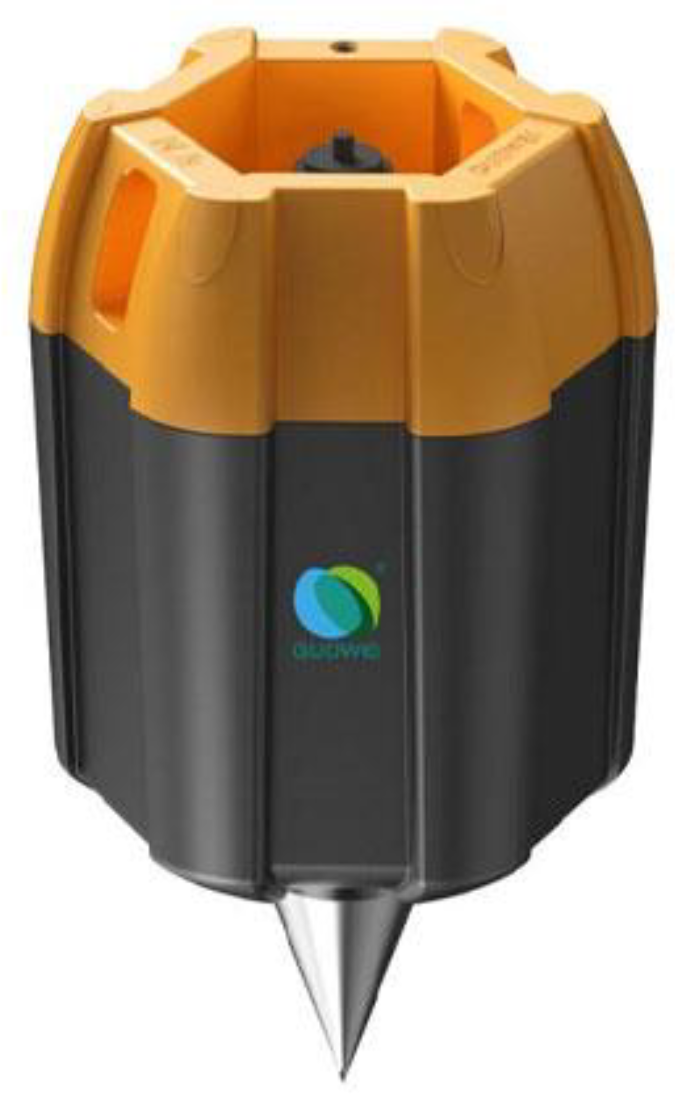
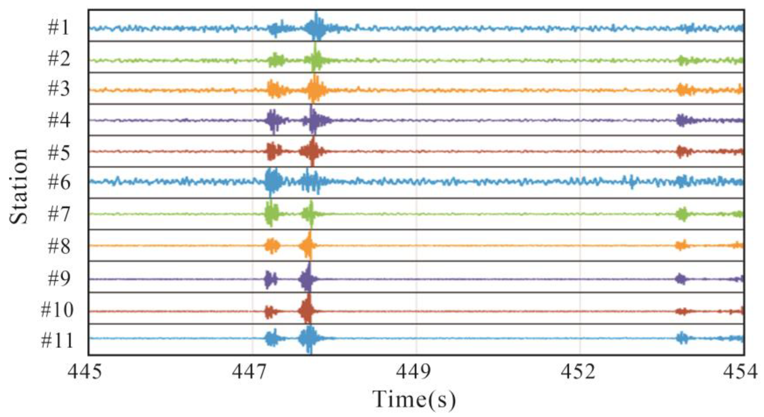
3.2. Instrument Consistency Test

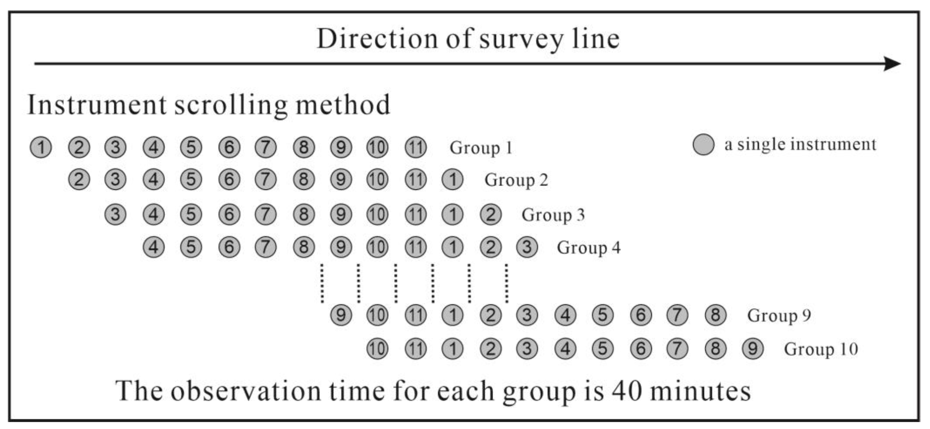
To ensure the reliability of experimental data, the consistency of each instrument should be ensured before data collection. In this experiment, 11 sets of GN309 remote real-time intelligent micromotion detectors were used. Prior to formal data collection, Hefei Guowei Electronics Co., Ltd., Hefei, China, conducted a unified consistency test. Figure 5 shows a GN309 remote real-time intelligent microtremor detector.

Table 1. GN309 detector parameters.

Name	Specifications
Natural frequency	2 Hz
Sensitivity	260 V/m/s
Frequency response range	0.1~1600 Hz
Open-circuit damping coefficient	0.7
Coil impedance	6400 Ω

shows the specifications of GN309. We placed all of the instruments in order and recorded the waveform within 10 min; in addition, a section of waveform record in the range of 445~454 s was intercepted from the server (Figure 6). It can be seen that the response trend and waveform consistency of each instrument in the same time period were good, ensuring that the consistency of the instrument met the requirements of fretting detection.

3.3. Array Layout

As the ESPAC method was adopted in this experiment, the requirements for array layout were more flexible. However, if the energy of the natural source surface wave was equal in all directions, a linear arrangement could be adopted, which is easier to implement in field work [18]. At the same time, the survey line was located around the village. If the array was arranged in two dimensions, the experimenters needed to enter the village to place instruments, and there are a lot of dangerous buildings in the village. Considering the actual terrain conditions and the safety of the technicians, a linear array was selected for this experiment.

According to the data provided by the mining party, the burial depth of Coal Seam #2 is roughly 410~420 m, so the exploration effect could be guaranteed if the exploration depth was 500 m. If the exploration depth is H, the number of each array is n and the spacing between geophones is d, the following formula should be met:

$$n=[H/(1.5~2.5)d]+1$$

(8)

We used 11 collection stations in total, so n is 11. In (8), we can deduce that the geophone spacing d should be set between approximately 20 and 33 m.

Due to the small number of acquisition stations in this experiment, in order to maintain a high detection resolution on the basis of meeting the exploration depth, the spacing between the acquisition stations was set as 20 m. The acquisition station could not cover the whole measuring line at one time, so the linear rolling acquisition method was adopted in this experiment [20]. This made use of the characteristics of the linear array and reused the data of the acquisition station on the linear array. It used eight acquisition stations to survey two micro-points each time. After one acquisition, it moved the two stations at the back of the line to the front for the rolling operation, effectively improving the working efficiency by more than double. On this basis, Hefei Guowei Electronics Co., Ltd., Hefei, China, in collaboration with the Seismological Research Institute of the China Seismological Bureau, further improved and perfected the acquisition method. By laying 20 acquisition stations in a straight line and surveying more than 10 micro-points at the same time, the data were reused to a greater extent, and the exploration efficiency was further improved to more than 10 times the original.

3.4. Data Acquisition

Before arranging the acquisition station, the instruments were sequenced and numbered to identify and intercept the fretting data by the post-processing software. The receiving point positions of all acquisition stations were determined by the longitude and latitude acquired by a GPS. The consistency of each receiving point was controlled by the internal synchronous clock of the GPS, and the error of each receiving point position was less than 10⁻¹ s. Each collection station separately collected experimental data and transmitted it to the computer terminal through a 4G signal.

Two survey lines were set up in this experiment: the WD1 line had 10 survey points, with a spacing of 20 m, a total length of 380 m and an actual exploration length of 190 m; the WD2 line had 8 measuring points, with a spacing of 20 m, a total length of 340 m and an actual exploration length of 170 m. Taking the WD1 line as an example, 11 acquisition stations were used to survey one point each time, and each acquisition and observation lasted for 40 min. After the acquisition, the station at the back of the line was moved to the front to realize the rolling acquisition (Figure 7).

4. Results and Discussion

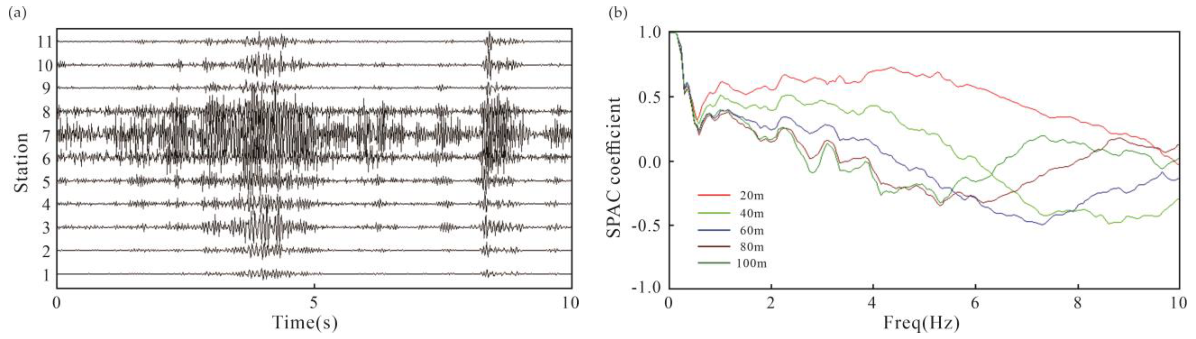
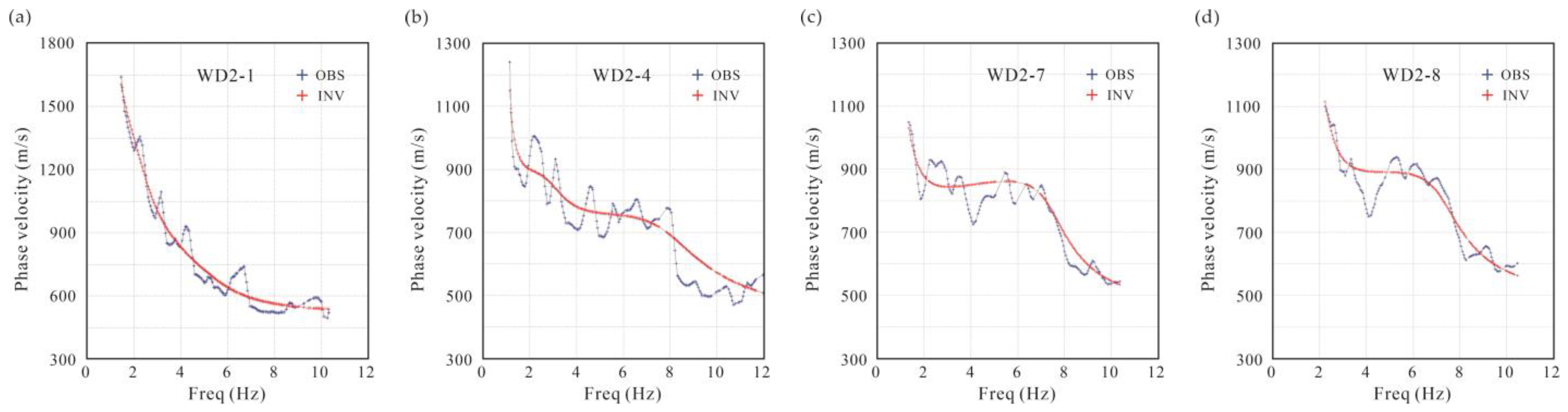
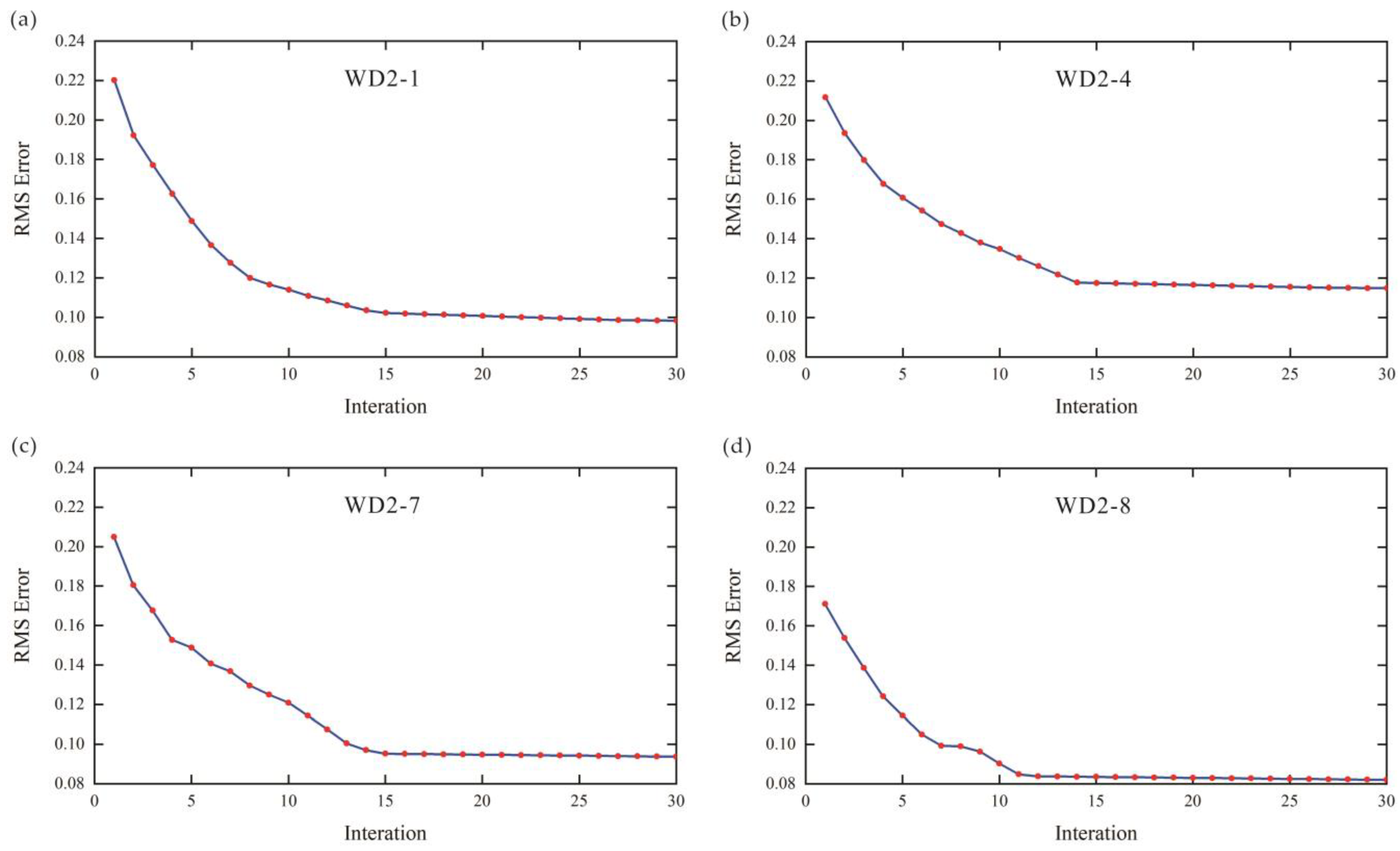
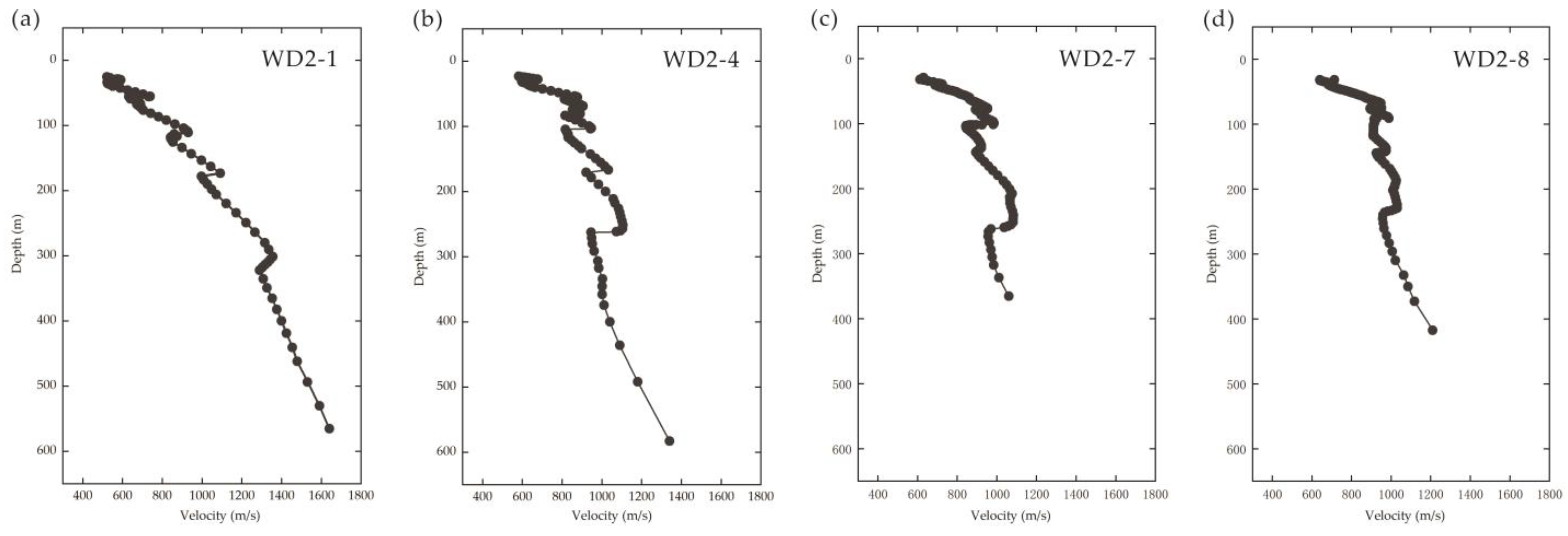
4.1. Data Processing Flow

After the consistency of all instruments reached the standard, we started to collect the data, and the collected data files were saved in an SG2 format. For the data processing of this experiment, we used the Surface Plus module in Canada’s Geogiga Seismic Pro software. Firstly, we needed to import the raw data of each measuring point into the Surface Plus module. Secondly, when setting up the observation system, considering that some acquisition stations may be affected by interfering objects, such as trees, gravel and abandoned building residues, and when the acquisition stations were placed in accordance with the specified coordinates, we needed to place the acquisition stations in deviation, with the placement deviation not exceeding 5 m. To ensure the reliability of the data results, the allowable deviation of the ESPAC calculation was set to 5%. Thirdly, we removed the interfering seismic traces, and calculated the dispersion spectrum of this point after setting the dispersion analysis parameters. Finally, we picked up the dispersion curve of the point manually. Since there were few borehole data in this area, the initial velocity model of the formation could be automatically generated when the dispersion curve of this point was inversed.

The relevant research on surface wave inversion shows that the surface wave inversion based on the genetic algorithm has a fast calculation speed, strong global search ability and much less dependence on the initial model than other linear inversion methods, so this algorithm was used in the inversion of the velocity model [19]. Based on Darwin’s theory of biological evolution, the genetic algorithm (GA) simulates the process of natural selection and biological evolution, and uses iterative processes such as coding, selection and transformation to solve the optimal solution, which has an advantage over the global nonlinear method [21].

We used the built-in GA method to invert the dispersion curve. The algorithm built into the software automatically determines the thickness and number of layers of the initial model according to the measured dispersion curve curvature. We set the population size to 128, the crossing probability to 95% and the variation probability to 9%, and obtained the apparent shear wave velocity and D-V curve of the point. Finally, we collected all the dispersion curves to obtain the underground velocity structure profile of the survey line.

Figure 8 shows a waveform record of the WD1-1 measuring point within 10 s. It can be seen from the figure that the data interference of the No. 6, 7 and 8 acquisition stations at this measuring point was large, so it was necessary to remove it from the seismic channels when calculating the dispersion spectrum, so as to ensure the reliability of the results.

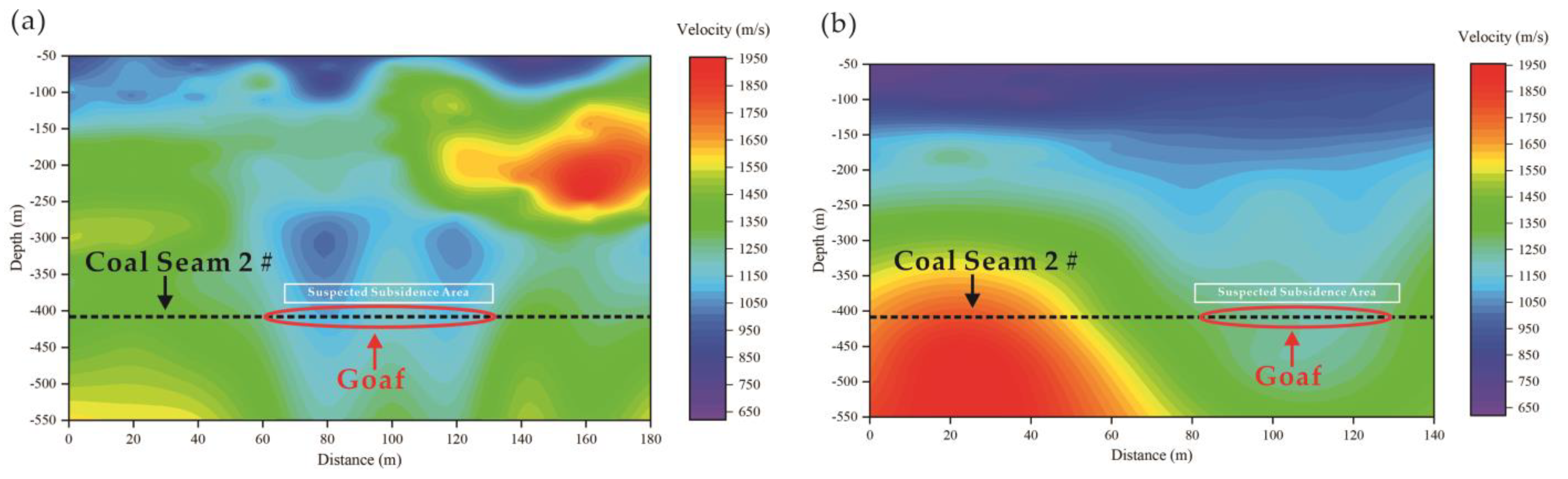
4.2. Interpretation of Achievements

The microtremor method is to divide the interface of the underground media according to the density and trend change in data points in the dispersion curve. Sparse data points indicate that the lithologic particle size is large, and dense data points indicate that the lithologic particle size is small. If the formation velocity suddenly changes or there is a low velocity interlayer, the dispersion curve at this position will have a zigzag inflection point [22].

Figure 9 shows the comparison between the dispersion data retrieved from some measuring points of the WD2 line and the actual observation data, and Figure 10 shows the change in the fitting mean square deviation of the dispersion curve with the number of iterations. It can be seen that the fitting effect of the dispersion curve was good. The initial model was automatically generated. Although it was somewhat different from the actual formation data, the initial value of the mean square error of dispersion curve fitting was small, and the target function converged quickly in the inversion process. The mean square error of 12~15 iterations was able to meet the inversion requirements.

By calculating the D-V observation curves of 18 exploration points in the survey area (Figure 11), we found that the effective detection depth was approximately 50~500 m and the velocity range was 400~1600 m/s. At some measuring points, the formation velocity changed obviously, and the velocity curves of the measuring points all jumped between approximately 300 and 400 m buried depth, with a zigzag inflection point.

In this experiment, data acquisition of 38 points was carried out, including 18 exploration points and 2 micro-measuring-lines. The following is the apparent shear wave velocity profile of the two survey lines (Figure 12). The black dotted line represents the position of Coal Seam #2. The red oval represents the position of the goaf. The white rectangular area represents the suspected subsidence area.

It can be seen from the apparent shear wave velocity profile of the WD1 line that there were two obvious low-speed areas within a buried depth of approximately 400 m and a distance of 40~60 m. The apparent shear wave velocity was lower than 1250 m/s, which may be caused by the goaf of Coal Seam #2. The WD1 line crossed two goaf areas of Coal Seam #2, which are shown as two low-speed areas on the profile map. Above Coal Seam #2 and within the buried depth of 300~400 m, the apparent shear wave velocity was also relatively low. The two sides of the seam were slightly thin and the middle was relatively thick, which may be related to the collapse of Coal Seam #2 caused by goaf ponding.

The detection results of the above two survey lines are in good agreement with the known goaf area of Coal Seam #2, and the resolution in the shallow part was fine. Especially in the transverse direction, the boundary of the goaf was basically consistent with the boundary of the apparent shear wave velocity profile of the micromotion detection. However, the overlying strata collapse caused by coal mining and the geological structure in the area varied, making the thickness of the low velocity layer significantly greater than the thickness of the coal seam. In terms of ground construction conditions, WD1 is arranged in a nearly north–south orientation, almost parallel to the terrain contour line, and the terrain is relatively flat. WD2 is arranged in a nearly east–west orientation, in which the terrain between WD2-1 and WD2-5 is relatively flat. WD2-6 and WD2-8 are arranged along the hillside, almost perpendicular to the terrain contour line, and the terrain elevation difference is large. From the detection results of the above two survey lines, it can be seen that in the vertical direction the resolution of the linear array in flat terrain was significantly higher than that in undulating terrain.

5. Conclusions

In this experiment, we used the microtremor detection method and linear array, extracted the dispersion curve by using the spatial autocorrelation method, obtained the apparent shear wave velocity profile of the underground medium through inversion, identified and verified the location of the goaf of Coal Seam #2 in the Nanling Coal Mine and inferred the collapse of the overlying strata caused by the water accumulation in the goaf, thus providing reference information for the next step of governance of the goaf.

• When a linear array is selected for microtremor exploration, If the number of acquisition stations cannot meet the requirements of one-time data observation, we can choose to deploy the linear array to collect data using rolling acquisition, so that the work efficiency can be greatly improved by reusing the data.
• Microtremor exploration is less affected by the environment, and the construction is simple and flexible. It is useful for field work, and the shallow strata are depicted more finely, which can make up for the shortcomings of other geophysical methods in shallow resolution.
• The layout of the microarray also includes a nested equilateral triangle and circular array. These two arrays require wide site conditions in the target area, but these two methods are not applicable to the topographic conditions of our experimental exploration area. The linear array and rolling acquisition method used in this study are suitable for use in poor terrain, which can shorten the time taken for array layout and improve construction efficiency, while ensuring the exploration effect. The shallow resolution of linear array is inferior to that of a nested equilateral triangle array and circular array. The layout of the array should also consider the site conditions in the construction area.

References

1. Xue, G.Q.; Cheng, J.L.; Zhou, N.N.; Chen, W.Y.; Li, H. Detection and monitoring of water-filled voids using transient electromagnetic method: A case study in Shanxi, China. Environ. Earth Sci. 2013, 70, 2263–2270. [Google Scholar] [CrossRef]
2. Qin, S.; Cheng, J.Y.; Hu, J.W.; Wu, H. Coal-seam-ground-seismic for advance detection of goaf and roadway. J. China Coal Soc. 2015, 40, 636–639. [Google Scholar]
3. Cai, G.T.; Sui, W.H.; Wu, S.L.; Wang, J.L.; Chen, J.X. On-Site Monitoring for the Stability Evaluation of a Highway Tunnel above Goaves of Multi-Layer Coal Seams. Appl. Sci. 2021, 11, 7383. [Google Scholar] [CrossRef]
4. Xv, X.C.; Chen, W.D.; Liu, W. Application of ground-penetrating radar and high-density electromagnetic method to prospecting obsolete mine. Rock Soil Mech. 2002, 23, 126–128. [Google Scholar]
5. Keiiti, A. Space and time spectra of stationary stochastic waves, with special reference to microtremors. Bull. Earthq. Res. Inst. 1957, 35, 415–456. [Google Scholar]
6. Capon, J. High-resolution frequency-wavenumber spectrum analysis. Proc. IEEE 1969, 57, 1408–1418. [Google Scholar] [CrossRef] [Green Version]
7. Okada, H. The Microtremor Survey Method; Society of Exploration Geophysicists: Tokyo, Japan, 2003; pp. 76–77. [Google Scholar]
8. Ohori, M.; Nobata, A.; Wakamatsu, K. A Comparison of ESAC and FK Methods of Estimating Phase Velocity Using Arbitrarily Shaped Microtremor Arrays. Bull. Seismol. Soc. Am. 2002, 92, 2323–2332. [Google Scholar] [CrossRef]
9. Fen, S.K. Array Microtremor Survey and Its Application to Civil Engineering. Chin. J. Rock Mech. Eng. 2003, 6, 1029–1036. [Google Scholar]
10. Ye, T.L. The Exploration Technique for Microtremor Array and Its Application. Earthq. Res. China 2004, 20, 47–52. [Google Scholar]
11. Xu, P.F.; Li, S.H.; Du, J.G.; Ling, S.Q.; Guo, H.L.; Tian, B.Q. Microtremor survey method: A new geophysical method for dividing strata and detecting the buried fault structures. Acta Petrol. Sin. 2013, 29, 1841–1845. [Google Scholar]
12. Tian, B.Q.; Xu, P.F.; Ling, S.Q.; Du, J.G.; Xu, X.Q.; Pang, Z.H. Application effectiveness of the microtremor survey method in the exploration of geothermal resources. J. Geophys. Eng. 2017, 14, 1283–1289. [Google Scholar] [CrossRef] [Green Version]
13. Huang, H.C.; Shih, T.H.; Hsu, C.T.; Wu, C.F. Estimation of Shear-Wave Velocity Structures in Taichung, Taiwan, Using Array Measurements of Microtremors. Appl. Sci. 2022, 12, 170. [Google Scholar] [CrossRef]
14. Ma, G.S. Mapping water-rich goaf utilizing microtremor survey methods. Prog. Geophys. 2022, 37, 1292–1300. [Google Scholar]
15. Xu, P.F.; Li, S.H.; Ling, S.Q.; Guo, H.L.; Tian, B.Q. Application of SPAC method to estimate the crustal S-wave velocity structure. Chin. J. Geophys. 2013, 56, 3846–3854. [Google Scholar]
16. Xu, P.F.; Ling, S.Q.; Li, C.J.; Du, J.G.; Zhang, D.M.; Xu, X.Q.; Dai, K.M.; Zhang, Z.H. Mapping deeply-buried geothermal faults using microtremor array analysis. Geophys. J. Int. 2012, 188, 115–122. [Google Scholar] [CrossRef]
17. Ling, S.; Okada, H. An Extended Use of the Spatial Autocorrelation Method for the Estimation of Geological Structure Using Microtremors. In Proceedings of the 89th SEGJ Conference, Nendo Shuki, Japan, 12–14 October 1993. [Google Scholar]
18. Liao, C.W.; Deng, T.; Ding, W.; Wang, H.; Tan, Y.Y.; Chen, W.M. On positioning way for array microtremor observation. J. Geod. Geodyn. 2007, 27, 61–64. [Google Scholar]
19. Li, N.; He, Z.Q.; Ye, T.L.; Fang, S.C. Test for comparison of array layout in natural source surface wave exploration. Acta Seismol. 2015, 37, 323–334+370. [Google Scholar]
20. Zhou, Z.Y.; Liao, W.L.; Li, J.G. Microtremor Survey Method Linear Array Rapid Processing. J. Geod. Geodyn. 2020, 40, 1097–1100. [Google Scholar]
21. Nagai, K.; O’neill, A.; Sanada, Y.; Ashida, Y. Genetic Algorithm Inversion of Rayleigh Wave Dispersion from CMPCC Gathers Over a Shallow Fault Model. J. Environ. Eng. Geophys. 2005, 10, 275–286. [Google Scholar] [CrossRef]
22. Zhang, B.X.; Xiao, B.X.; Yang, W.J.; Cao, S.Y.; Mou, Y.G. Mechanism of zigzag dispersion curves in Rayleigh exploration and its inversion study. Chin. J. Geophys. 2000, 43, 557–567. [Google Scholar] [CrossRef]
Figure 1. Illustration of the single-circle observation array for the SPAC method.
Applsci 13 00466 g001
Figure 2. Micro-movement irregular observation array: (a) L-shaped array; (b) triangular array; and (c) cross array.
Applsci 13 00466 g002
Figure 3. The location of the survey area and the arrangement of the array.
Applsci 13 00466 g003
Figure 4. Layout of measuring points and goaf scope of Coal Seam #2.
Applsci 13 00466 g004
Figure 5. GN309 remote real-time intelligent microtremor detector.
Applsci 13 00466 g005
Figure 6. Waves of each seismometer in huddle test.
Applsci 13 00466 g006
Figure 7. Schematic diagram of instrument rolling.
Applsci 13 00466 g007
Figure 8. Two sets of parameters of WD1-1: (a) an example of the vertical-component records; (b) SPAC coefficients.
Applsci 13 00466 g008
Figure 9. Dispersion curve of some measuring points of WD2 line. (a) the dispersion curve of WD2-1; (b) the dispersion curve of WD2-4; (c) the dispersion curve of WD2-7; and (d) the dispersion curve of WD2-8.
Applsci 13 00466 g009
Figure 10. The change in fitting mean square deviation of dispersion curve of some measuring points of WD2 line with the number of iterations: (a) the RMS error of WD2-1; (b) the RMS error of WD2-4; (c) the RMS error of WD2-7; and (d) the RMS error of WD2-8.
Applsci 13 00466 g010
Figure 11. D-V curves of each measurement point of WD2 line: (a) the DV curve of WD2-1; (b) the DV curve of WD2-4; (c) the DV curve of WD2-7; and (d) the DV curve of WD2-8.
Applsci 13 00466 g011
Figure 12. Apparent shear wave velocity profiles of two lines: (a) the shear wave velocity profile of WD1 line; and (b) the shear wave velocity profile of WD2 line.
Applsci 13 00466 g012