Research on Short-Term Traffic Flow Combination Prediction Based on CEEMDAN and Machine Learning

Abstract

Traffic flow has the characteristics of randomness, complexity, and nonlinearity, which brings great difficulty to the prediction of short-term traffic flow. Based on considering the advantages and disadvantages of various prediction models, this paper proposes a short-term traffic flow prediction model based on complete ensemble empirical mode decomposition with adaptive noise (CEEMDAN) and machine learning. Firstly, CEEMDAN is used to decompose the original traffic flow time series to obtain multiple component sequences with huge complexity differences. In order to measure the complexity of each component sequence, the permutation entropy of each component sequence is calculated. According to the permutation entropy, the component sequence is divided into three types: high-frequency components, intermediate-frequency components, and low-frequency components. Secondly, according to the different volatility of the three types of components, the high-frequency components, intermediate-frequency components, and low-frequency components are predicted by long short-term memory (LSTM), support vector machine (SVM), and k-nearest neighbor (KNN), respectively. Finally, the accurate traffic flow prediction value can be obtained by the linear superposition of the prediction results of the three component prediction models. Through a measured traffic flow data, the combined model proposed in this paper is compared to the binary gray wolf algorithm–long short-term memory (BGWO-LSTM) model, the improved gray wolf algorithm–support vector machine (IGWO-SVM) model, and the KNN model. The mean square error (MSE) of the combined model is less than that of the BGWO-LSTM model, the IGWO-SVM model, and the KNN model by 41.26, 44.98, and 57.69, respectively. The mean absolute error (MAE) of the combined model is less than that of the BGWO-LSTM model, the IGWO-SVM model, and the KNN model by 2.33, 2.44, and 2.70, respectively. The root mean square error (RMSE) of the combined model is less than that of the BGWO-LSTM model, the IGWO-SVM model, and the KNN model by 2.89, 3.11, and 3.80, respectively. The three error indexes of the combined model are far smaller than those of the other single models. At the same time, the decision coefficient (R²) of the combined model is also closer to 1 compared to the other models, indicating that the prediction result of the combined model is the closest to the actual traffic flow.

1. Introduction

Accurate short-term traffic flow is the premise of the efficient operation of an intelligent transportation system. The process of estimating traffic flow data for the next time period by using predictive algorithms to analyze existing traffic data is called traffic flow prediction. Short-term traffic flow forecasting requires quick feedback, and its time span is generally considered to be no more than 15 min [1]. The evolution of road traffic operating conditions is a dynamic random change process, and its changes are affected by many natural and human factors, such as weather changes and sudden traffic accidents, which makes the traffic operation state strongly random and poses a huge challenge to traffic flow prediction [2]. Because the short-term traffic flow prediction interval is relatively short, the prediction result is more obviously affected by random interference factors, so the difficulty of realizing the real-time prediction of short-term traffic flow is much greater than that of medium-term and long-term prediction of traffic flow. However, in order to realize the real-time guidance of traffic in intelligent transportation systems, it is necessary to publish traffic information in good time, which requires the study of traffic characteristics on short-term scales [3].

2. Current Research Status

Short-term traffic flow prediction is a trending topic in the field of transportation research. More scholars are starting their research in this area very early. According to different research theories, the research can be roughly divided into three categories.

2.1. Predictive Model Based on Mathematical Statistical Analysis

Forecasting models based on mathematical statistical analysis have an important assumption—that historical data and prediction results have exactly the same characteristics. These kinds of forecasting models mainly include the Kalman filter prediction method, the time series analysis forecasting method, the historical average forecasting method, and so on. Since Kalman [4] proposed Kalman filtering in 1960 [3], due to its excellent performance and good effect, Kalman filtering and its improved algorithms have been widely used in modern projects, such as control, finance, communication, inertial guidance, fault detection, and signal processing. Okutani et al. [5] were the first to verify that Kalman filtering has a good predictive effect on short-term traffic flow. Shen Leixiao [6] and other scholars used the dataset of Xuzhou National–Provincial Highway to verify the short-term traffic flow prediction model based on Kalman filtering. Among many time series forecasting models modeled by parametric modeling, ARIMA [7] is the most widely used. Kumar et al. [8] proposed an ARIMA model that takes into account seasonality. Historical average prediction is the earliest forecasting method applied to transportation systems, but the accuracy of prediction is difficult to guarantee, especially when there is an emergency on the road. As a result, the historical averaging method cannot be applied to the increasingly complex modern transportation system [9].

2.2. Prediction Model Based on Intelligence Theory

The intelligent theory prediction model is the establishment of machine learning theory, neural network theory, and deep learning theory applied to a short-term traffic flow prediction model. Hu et al. [10] used an improved particle swarm algorithm to optimize the relevant parameters of the support vector machine, aiming at the problem that noise in the original traffic flow data led to the degradation of model accuracy, which proved that the prediction effect can still be good when the traffic data is noisy. Wang et al. [11] used principal component analysis (PCA) to extract the historical data of core traffic parameters of traffic flow data in Baltimore, USA and then applied the KNN algorithm to predict the state values of core traffic parameters, including traffic flow and traffic speed in the near future. Mao Yunxiang et al. [12] proposed a stochastic forest algorithm that combines multi-node splitting to solve the problem of the poor applicability of traditional decision trees due to the single-split node. Di et al. [13] proposed using the firefly algorithm (FA) to optimize the weights and biases in the BP neural network and constructed the FA–BPNN model. Zhao et al. [14] proposed a parallel radial basis neural network (RBFNN) model to predict traffic flow in a certain area of the city. Wen Huiying et al. [15] used genetic algorithms (GA) to perform the hyperparameter optimization of long short-term memory neural network (LSTM) models, and the GA-LSTM model had good predictive performance. Zhang et al. [16] considered the spatiotemporal correlation of the data and proposed a new deep learning framework called the attention map convolutional sequence-to-sequence model.

2.3. Prediction Model Based on a Combination Forecasting

In 1969, Bates et al. [17] first proposed the concept of combined models, which combine more than two models to predict traffic flow for the complex traffic conditions of different roads in different cities, which can overcome the limitations of a single prediction model to the greatest extent and organically combine the advantages of a single model. Wang Jian et al. [18] used Bayesian networks to combine BP neural network models, differentially integrated moving average autoregressive models based on wavelet analysis, and BP neural network models based on wavelet analysis to make them more accurate than single prediction models. Li et al. [19] developed a deep learning-based approach that includes two single models, CNN and LSTM, for real-time traffic flow prediction at road intersections. Xia et al. [20] proposed an LSTM-weighted model that combines a normal distribution with a time window to enhance the ability to predict traffic flows. Zhou et al. [21] combined LSTM and SVR to construct a short-term traffic flow prediction model, and the results show that the accuracy of the prediction model was higher than that of LSTM and CNN.

3. Methods and Principles

3.1. Complete Ensemble Empirical Mode Decomposition with Adaptive Noise (CEEMDAN)

Torres et al. [22] first proposed the empirical modal decomposition algorithm of adaptive noise-assisted sets, which continuously averages new signals by adding adaptive Gaussian white noise on the basis of the EMD algorithm. It not only solves the problem of modal aliasing but also avoids noise interfering with the original signal, making the signal decomposition more thorough. The decomposition process of CEEMDAN is as follows:

(1) The new signal sequence $x_i\left(t\right)$ is obtained by adding the adaptive noise of n times the same length to the original signal sequence $x\left(t\right)$. The new sequence is decomposed N times with EMD, and the average value is the first eigenmodal function IMF₁. The formula is described as follows:

$$x_i\left(t\right)= x\left(t\right)+\epsilon {\omega }_i\left(t\right)$$

(1)

$${\mathrm{IMF}}_1\left(t\right)=\frac{1}{N}{\displaystyle \sum _{i=1}^N{\mathrm{IMF}}_{1i}\left(t\right)}$$

(2)

where $\epsilon$ is the adaptive coefficient and ${\omega }_i\left(n\right)$ is the noise sequence.

(2) The first margin sequence $r_1\left(t\right)$ is calculated as follows:

$$r_1\left(t\right)=x\left(t\right)-{\mathrm{IMF}}_1\left(t\right)$$

(3)

(3) On the basis of (2), the second eigenmodal function IMF₂ is calculated as follows:

$${\mathrm{IMF}}_2\left(t\right)=\frac{1}{N}{\displaystyle \sum _{i=1}^N{\mathrm{IMF}}_1}\left(r_1\left(t\right)+{\epsilon }_1{\mathrm{IMF}}_1\left(\epsilon {\omega }_i\left(t\right)\right)\right)$$

(4)

(4) Repeat the calculation until the k + 1 stage and the margin sequence $r_k\left(t\right)$ of the kth stage and the k + 1 eigenmodal component IMF_k+1 are obtained as follows:

$$r_k\left(t\right)=r_{k-1}\left(t\right)-{\mathrm{IMF}}_k\left(t\right)$$

(5)

$${\mathrm{IMF}}_{k+1}\left(t\right)=\frac{1}{N}{\displaystyle \sum _{i=1}^N{\mathrm{IMF}}_1}\left(r_1\left(t\right)+{\epsilon }_k{\mathrm{IMF}}_k\left({\omega }_i\left(t\right)\right)\right)$$

(6)

(5) Repeat the above steps until the extreme point of the margin sequence is not greater than 2, then stop the EMD algorithm. Then the original sequence can be decomposed into K eigenmodal functions and a margin sequence through the above steps [23]:

$$x\left(t\right)={\displaystyle \sum _{i=1}^K{\mathrm{IMF}}_K\left(n\right)+R\left(n\right)}$$

(7)

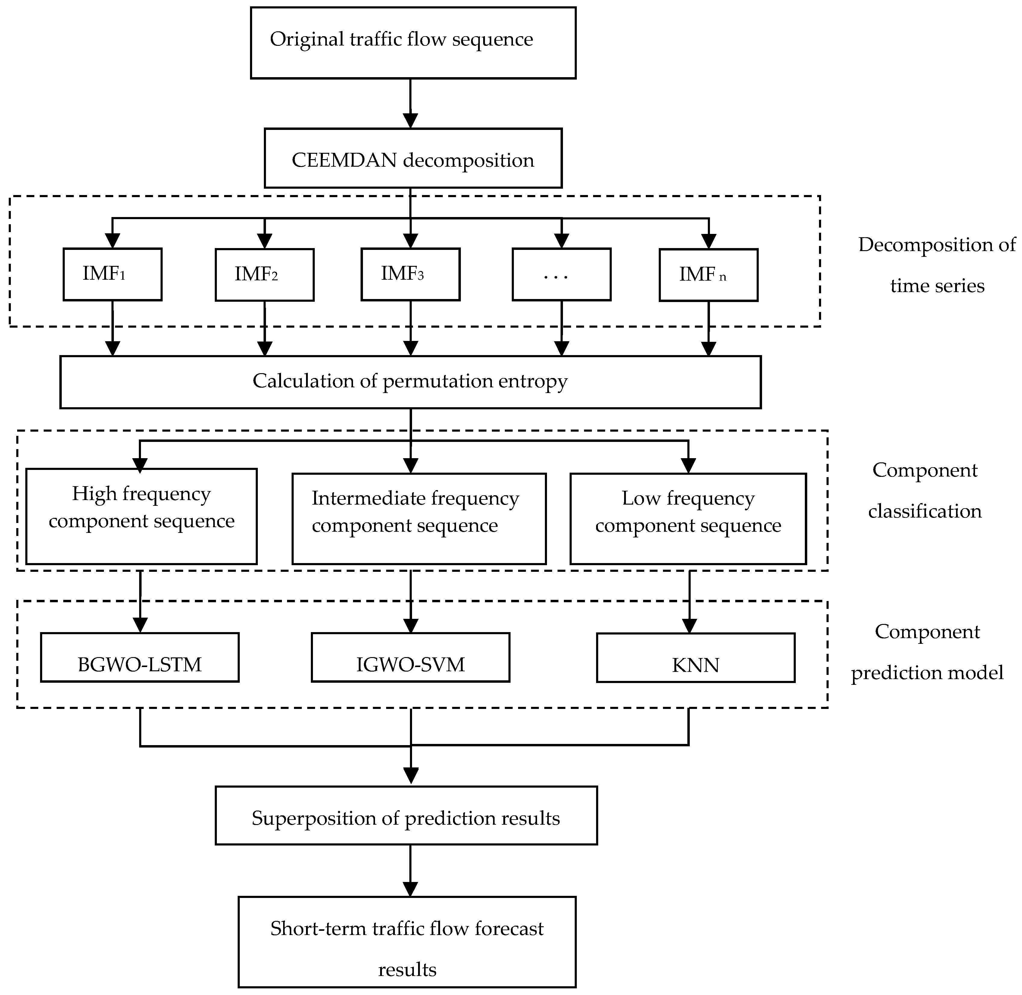
3.2. IMF Classification Based on Permutation Entropy

The permutation entropy (PE) algorithm was first proposed by Christoph Bandt et al. [24] in 2002 and can effectively detect mutations and randomness in complex dynamical systems. The basic principle of the algorithm is as follows:

(1) There is an existing set of time series $\left\{X\left(i\right),i=1,2,\cdots ,n\right\}$, and the phase space reconstruction of this set of one-dimensional time series data is obtained as follows:

$$\left[\begin{array}{cccc}x\left(1\right)& x\left(1+\tau \right)& \cdots & x\left(1+\left(m-1\right)\tau \right)\\ ⋮& ⋮& \cdots & ⋮\\ x\left(j\right)& x\left(j+\tau \right)& \cdots & x\left(j+\left(m-1\right)\tau \right)\\ ⋮& ⋮& \cdots & ⋮\\ x\left(k\right)& x\left(k+\tau \right)& \cdots & x\left(k+\left(m-1\right)\tau \right)\end{array}\right]$$

(8)

where m represents the embedded dimension, $\tau$ is the delay time, and j = 1, 2, …, k.

(2) If each row of the reconstructed matrix is treated as a component, there are a total of k components in the matrix, and each component is arranged in ascending order according to the numerical size, with:

$$x\left(i+\left(j_1-1\right)\tau \right)\le x\left(i+\left(j_2-1\right)\tau \right)\le \cdots \le x\left(i+\left(j_m-1\right)\tau \right)$$

(9)

where $j_1$, $j_2,\cdots$, $j_m$ represents the ordinal number of the column in which each component is located. Thus, for each row vector of the reconstructed matrix, it can be seen as a set of sequences $S\left(l\right)$:

$$S\left(l\right)=\left\{j_1, j_2,\cdots , j_m\right\}$$

(10)

where $l=1,2,\cdots ,k$, and $k\le m!$, and there are a total of $m!$ different mapping symbols in the m-dimensional space. Calculate the probability of each symbol appearing separately, $P_1,P_2,\cdots ,P_k$, and define the PE of the time series $\left\{X\left(i\right),i=1,2,\cdots ,n\right\}$ as in the form of Shannon entropy:

$$H_p\left(m\right)=-{\displaystyle \sum _{g=1}^l{P}_{g}ln{P}_g}$$

(11)

where $P_g=\frac{1}{m!}$, $H_p\left(m\right)$ has the maximum value $ln\left(m!\right)$, so for convenience, the $H_p\left(m\right)$ normalization process will be carried out:

$$H_{PE}\left(m\right)=\frac{H_p\left(m\right)}{ln\left(m!\right)}$$

(12)

Obviously, the value of $H_{PE}\left(m\right)$ in the formula is 0 to 1, and the size of the value of $H_{PE}\left(m\right)$ can be used to measure the degree of randomness of the time series. The larger the value of $H_{PE}\left(m\right)$, the higher the degree of randomness of the time series. Conversely, the smaller the value of $H_{PE}\left(m\right)$, the lower the degree of randomness of the time series.

4. Combined Model Construction and Case Analysis Based on CEEMDAN and Machine Learning

Aiming at the shortcomings of low prediction accuracy and the hysteresis of the prediction results of a single model, the authors of this paper analyzed the traffic flow sequence to find the inherent characteristics of the traffic flow sequence, and constructed a short-term traffic flow combination prediction model based on CEEMDAN and machine learning.

4.1. Short-Term Traffic Flow Combination Model Based on CEEMDAN

The core idea of the short-term traffic flow prediction model based on CEEMDAN is “primitive traffic flow—decomposition—traffic flow component sequence classification—establishment of component sequence prediction model—superposition prediction result”. Firstly, the traffic flow time series is decomposed into multiple component sequences with CEEMDAN, and then by calculating the permutation entropy of each component sequence, the component sequence is divided into high-frequency, medium-frequency, and low-frequency component sequences according to the size of the permutation entropy. Then, three different component prediction models are constructed according to the fluctuation characteristics and frequency characteristics of the three component sequences. Finally, the prediction results of each model can be superimposed to obtain accurate traffic flow prediction results.

4.1.1. Construction of BGWO-LSTM Models

High-frequency component sequences have strong randomness, volatility, and nonlinearity. Specifically, these high-frequency component sequence data have many large fluctuations in a very short time. Because long short-term memory (LSTM) has a strong nonlinear mapping ability and can fit complex data, LSTM was selected to predict the high-frequency components. The accuracy of the LSTM model is greatly related to four discrete parameters, including the historical data step (look back, hereafter referred to as lb), the number of hidden network layers (lstm nets, hereafter referred to as ls), training sessions (epochs, hereafter referred to as ep), and dropout (dp). The binary gray wolf algorithm (BGWO) was selected to optimize these four parameters to construct a high-frequency component prediction model of BGWO-LSTM. The high-frequency component prediction process based on BGWO-LSTM is shown in Figure 1, which is composed of four modules, including data preprocessing, discrete parameter optimization, neural network training, and data prediction.

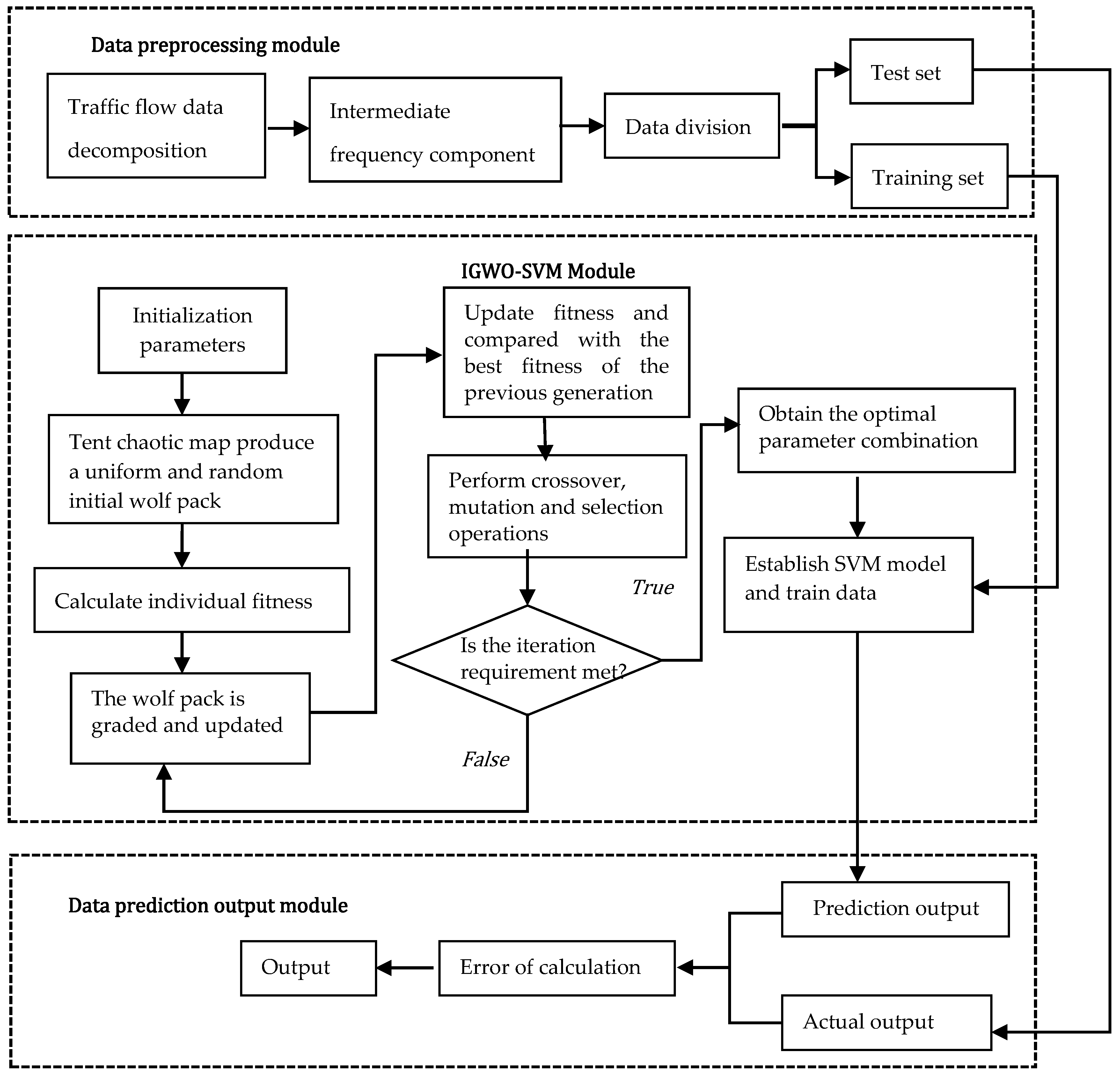
4.1.2. Construction of the IGWO-SVM Model

After using CEEMDAN to decompose the traffic flow sequence, the intermediate-frequency component sequence is selected according to the size of the permutation entropy. The volatility, randomness, and nonlinearity of the intermediate-frequency component sequences are not as strong as those of the high-frequency components. Because the support vector machine has a good nonlinear mapping ability, and at the same time, the theory of the support vector machine is mature and the training time is much shorter than that of the neural network, the support vector machine was selected to construct the intermediate-frequency component sequence prediction model.

In order to build an accurate intermediate-frequency component sequence prediction model, the improved gray wolf algorithm (IGWO) was used to optimize the parameters of the support vector machine (SVM) and establish an IGWO-SVM model. The IGWO-SVM model uses cross-validation to divide the training set into five folds and determine the value range of parameter C and parameter γ from 0.01 to 100. Through the excellent ability of the IGWO to deal with continuous optimization problems, the combination of C and γ with the best performance in the training set is found. The best combination of parameters is applied to the support vector machine prediction so as to improve the prediction accuracy. The flowchart of the model is shown in Figure 2.

4.1.3. Construction of KNN Models

The low-frequency component sequence fluctuates smoothly, the data change amplitude is small, the principle of k-nearest neighbor (KNN) model is simple and easy to use, and its prediction mainly depends on the adjacent K samples. In contrast, the neural network gradually approaches the true value through the backpropagation of error and does not spend a lot of time looking for hyperplanes, such as the support vector machine, which will greatly reduce the computational complexity. The flowchart of the KNN prediction model is shown in Figure 3 using the five-fold cross-validation method to solve the optimal hyperparameter K and the KNN prediction model.

4.1.4. A Combined Model Based on CEEMDAN and Machine Learning

Each forecasting model has its own strengths and weaknesses for different kinds of data. In order to maximize the advantages of each component prediction model and enhance the generalization ability of the model, this paper proposes a combined model based on CEEMDAN and machine learning. The prediction steps for this combined forecasting model are as follows:

Step 1: CEEMDAN can accurately decompose the characteristics of time series, and decompose short-term traffic flow sequences into multiple component sequences with good performance;

Step 2: The sample entropy of each component sequence is calculated, and the random characteristics of each component sequence are measured by the size of the sample entropy. The component sequences are divided into high-frequency components, intermediate-frequency components, and low-frequency components according to the size of the PE value;

Step 3: Since LSTM has strong nonlinear mapping ability, LSTM is used to predict the high-frequency component sequence of traffic flow with strong randomness, volatility, and nonlinearity. In order to improve the accuracy of the model, on the basis of LSTM, BGWO is introduced to optimize the hyperparameters, and the BGWO-LSTM model is established. Because SVM has a strong learning ability and fast training speed for nonlinear data, SVM is used to predict the intermediate-frequency component sequence of traffic flow. At the same time, in order to further improve the performance of the model, the IGWO is introduced on the basis of SVM to optimize the parameters, and the IGWO-SVM model is established. The KNN model has the advantages of simple structure, mature theory, and short training time. KNN is used to predict the low-frequency component sequence of traffic flow, which is relatively stable and does not have strong variation;

Step 4: The prediction results of each high-frequency component, intermediate-frequency component, and low-frequency component are linearly superimposed to obtain accurate traffic flow prediction results.

The flowchart of the short-term traffic flow combination model based on CEEMDAN and machine learning is shown in Figure 4.

4.2. Case Studies

In order to verify the superiority of the short-term traffic flow prediction model based on CEEMDAN and machine learning proposed in this paper, real traffic flow data were used to train the model, and the combined model in this paper was compared with the prediction results of the LSTM model, the IGWO-SVM model, and the KNN model to verify the performance of the combined model and the three single models.

4.2.1. Data Sources

The traffic flow experimental data used in this article came from the PeMS system of the California Department of Transportation, which has used advanced induction coil detection technology to record traffic data for more than 20 years, since 2000, using more than 45,000 sensors in some sections of California. These advanced sensors collect data every 30 s. The authors selected the traffic flow data on a total of 5 days on the main road of a city recorded by 308,512 sensors from 7 October 2019 to 11 October 2019, with a data recording interval of 5 min and a total of 1440 traffic flow data (1152 data from the first 4 days as the training set, and 288 data on the last day as the test set). The authors only studied traffic flow, so some of the data after the redundant information were omitted are shown in

Table 1. Partial traffic flow data.

Time	Traffic Flow/Vehicle	Time	Traffic Flow/Vehicle
7 October 2019 00:00:00	43	7 October 2019 01:05:00	38
7 October 2019 00:05:00	47	7 October 2019 01:10:00	41
7 October 2019 00:10:00	42	7 October 2019 01:15:00	38
7 October 2019 00:15:00	40	7 October 2019 01:20:00	36
7 October 2019 00:20:00	43	7 October 2019 01:25:00	38
7 October 2019 00:25:00	45	7 October 2019 01:30:00	42
7 October 2019 00:30:00	38	7 October 2019 01:35:00	39
7 October 2019 00:35:00	40	7 October 2019 01:40:00	36
7 October 2019 00:45:00	36	7 October 2019 01:45:00	36
7 October 2019 00:50:00	36	7 October 2019 01:50:00	36
7 October 2019 00:55:00	43	7 October 2019 01:55:00	40
7 October 2019 01:00:00	38	7 October 2019 02:00:00	38

.

4.2.2. Data Preprocessing

The authors selected a time series of traffic flows for five consecutive days, as shown in Figure 5. It can be seen from the traffic flow time series curve chart that the traffic flow data do not form a gentle curve but fluctuate significantly with time changes. The traffic flow suddenly increased or decreased at some time points, showing strong randomness. At the same time, the trends of the traffic flows were similar over the course of the days, showing the cyclical nature of traffic flows.

For the existing traffic flow data, CEEMDAN was used for decomposition, and the white noise of 500 sets of standard deviations of 0.2 was added. The decomposition result is shown in Figure 6. As can be seen in Figure 6, the original traffic flow was decomposed into eight well-performing component sequences, which show the frequency and amplitude changes of the traffic flow sequence. In the figure, from top to bottom, the frequency of the component sequence gradually decreases, and the amplitude gradually decreases. IMF₁ has the largest fluctuation and shortest period, and IMF₈ has the smallest fluctuation, the longest period, and a certain degree of stationarity.

In order to measure the decomposition effect of CEEMDAN, the reconstruction error after the decomposition of traffic flow was calculated. Figure 7 shows the reconstruction error. As can be seen in the figure, the maximum reconstruction error does not exceed 6 × 10⁻¹⁴. The reconstruction error is extremely small and not enough to have an impact on the prediction results and can be ignored.

In order to accurately predict the sequence of different traffic flow components, the PE values of each IMF component obtained from the decomposition analysis were calculated. In the calculation of the PE values, the embedded dimension m and the delay time $\tau$ affected the sizes of the PE values. The embedded dimension m was 6 and the delay time $\tau$ was 1. The calculation results for each IMF component are shown in

Table 2. Permutation of entropy values by IMF component.

Component Sequence	IMF1	IMF2	IMF3	IMF4	IMF5	IMF6	IMF7	IMF8
PE	0.9950	0.8677	0.6898	0.5162	0.4203	0.4017	0.3931	0.0374

and Figure 8.

As can be seen in Table 2 and Figure 8, the permutation entropy of IMF 1 is the largest, the permutation entropy of IMF8 is the smallest, and as the component sequence increases, the permutation entropy value gradually decreases, indicating that the randomness and complexity of the time series component sequence gradually decrease. The permutation entropy values of IMF₁, IMF₂, IMF₃, and IMF₄ are between 0.5 and 1.0, indicating that these four component sequences have strong randomness and complexity, and they are regarded as high-frequency component sequences. The permutation entropy values of IMF₅, IMF₆, and IMF₇ are between 0.3 and 0.5, indicating that the randomness and complexity of these three components are not high, and they are regarded as intermediate-frequency components. The permutation entropy value of IMF8 is between 0 and 0.1, indicating that the randomness and complexity of the component sequence are weak, and it is listed as a low-frequency component. The classification of the component sequences provided a basis for the construction of the subsequent combined models.

4.2.3. Outcome Evaluation Indicators

The establishment of the outcome evaluation indicators is an indispensable part of traffic flow forecasting, and its significance is as follows:

(1) When the traffic flow of a certain section of the road is predicted, the overall advantages and disadvantages of the prediction results can be directly reflected, and the purpose of verifying the validity of the model is achieved;

(2) When we use different models to predict traffic flow, we can also visually compare the prediction effects of different models through evaluation indicators so as to quickly judge the advantages and disadvantages of the prediction models.

In this study, the short-term traffic flow prediction model was evaluated by the mean squared error (MSE), the mean absolute error (MAE), the root mean square error (RMSE), and the decision coefficient (R²) [25]. The calculation formula is as follows:

$$E_{MSE}=\frac{1}{N}{\displaystyle \sum _{i=1}^N{(y_i-\stackrel{\wedge }{y_i})}^2}$$

(13)

$$E_{MAE}=\frac{1}{N}{\displaystyle \sum _{i=1}^N\left|y_i-\stackrel{\wedge }{y_i}\right|}$$

(14)

$$E_{RMSE}=\sqrt{\frac{1}{N}{\displaystyle \sum _{i=1}^N{(y_i-\stackrel{\wedge }{y_i})}^2}}$$

(15)

$$R^2=1-\frac{\frac{1}{N}{\displaystyle \sum _{i=1}^N{(y_i-\stackrel{\wedge }{y_i})}^2}}{\frac{1}{N}{\displaystyle \sum _{i=1}^N{(\overline{y_i}-y_i)}^2}}$$

(16)

In the above equation, $E_{MSE}$ is the mean square error, $E_{MAE}$ is the mean absolute error, $E_{RMSE}$ is the root mean square error, $R^2$ is the decision coefficient, N is the total predicted time length, and $y_i$, ${\stackrel{\wedge }{y}}_{i },$ and $\overline{ y_i}$ are, respectively the measured value, predicted value, and the average value of traffic flow. The smaller the values of $E_{MSE}$, $E_{MAE},$ and $E_{RMSE}$, and the smaller the deviation between the predicted results and the actual traffic data, the better the model performance. R² is the correlation between the prediction results and the actual results, and its value is between 0 and 1. The closer it is to 1, the better the fitting regression effect is and the better the model is. Therefore, the optimal prediction model should simultaneously meet the two conditions of the minimum error and the maximum decision coefficient.

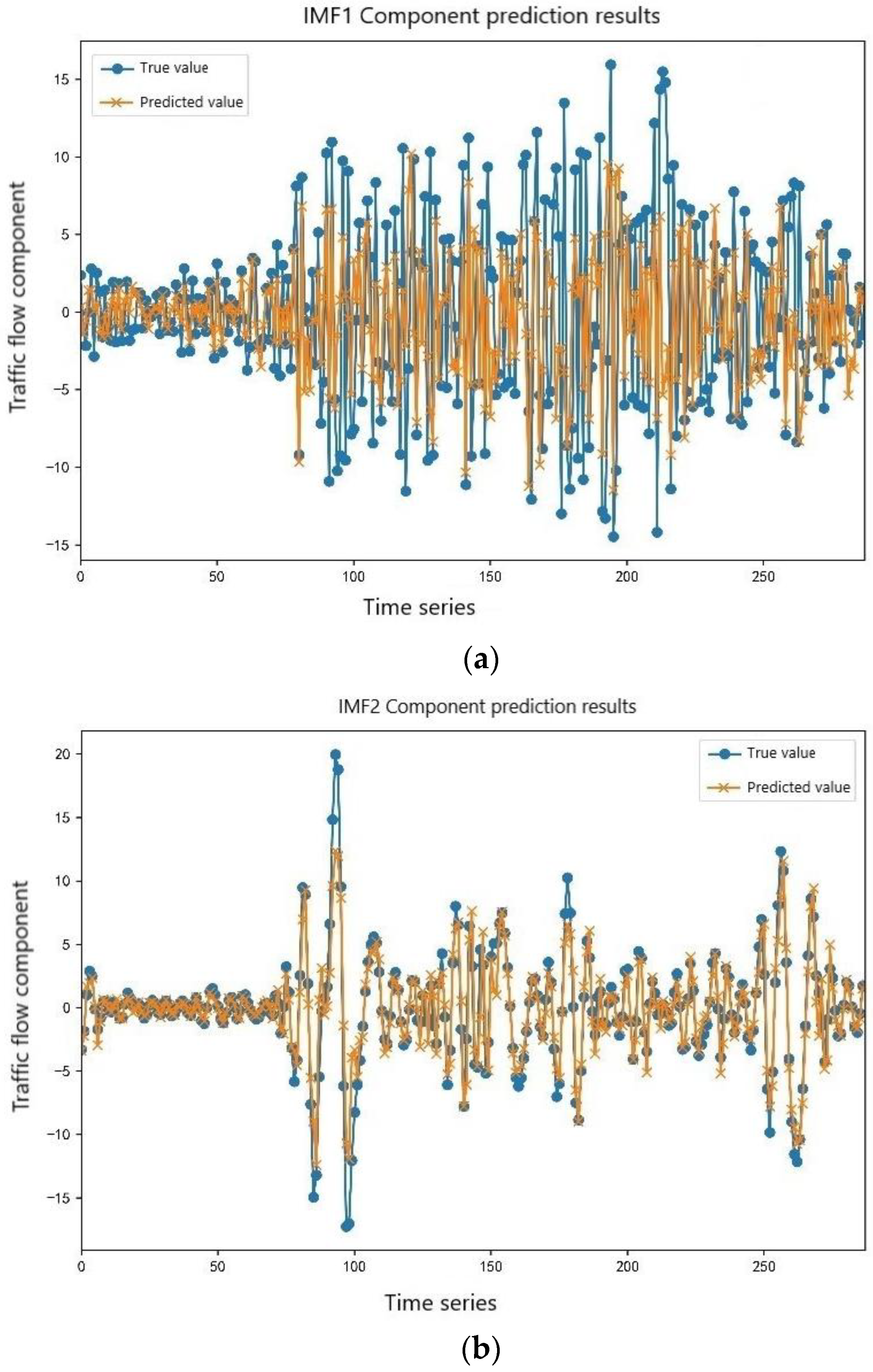
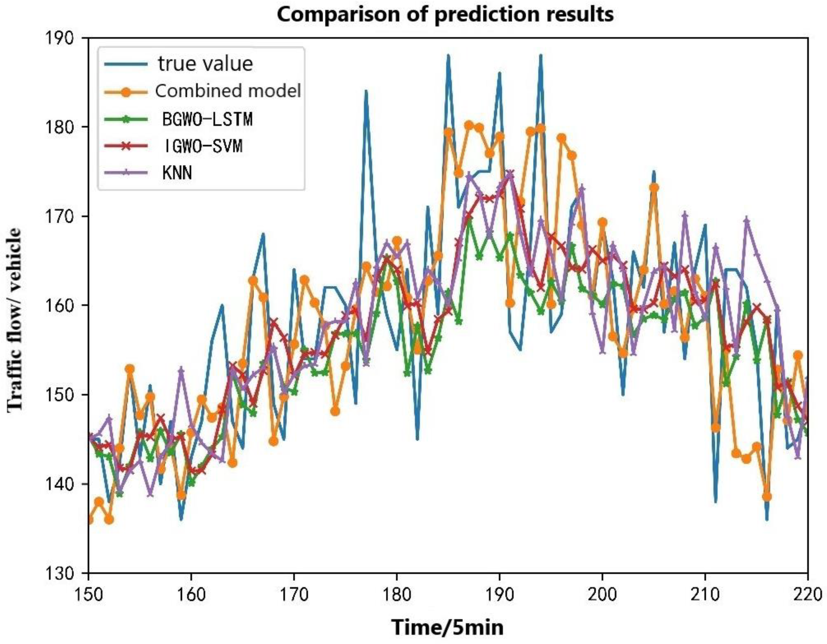
4.2.4. Comparative Analysis of Results

Due to the strong nonlinear mapping ability of the long short-term memory neural network and the strong randomness and volatility of the four high-frequency component sequences of IMF₁, IMF₂, IMF₃, and IMF₄, the BGWO-LSTM model was selected for prediction in this study. The initial population number was set to 30, the maximum number of iterations was 100, the lb value was 3~20, the step size was 1, the ls value was 5~50, and the step size was 5. The ep value was 50 to 300, the step size was 10, the dp value was 0.3 to 0.61, and the step size was 0.01. The high-frequency component prediction is shown in Figure 9.

In Figure 9, it can be seen that IMF₁ had the highest frequency, the strongest volatility, the greatest difficulty in forecasting, and the largest error in prediction. As the component sequence grew, the degree of fluctuation of the data decreased, the error of prediction was gradually reduced, and IMF₄ achieved a good fitting effect.

Due to the good nonlinear mapping ability of support vector machine, the three intermediate-frequency component sequences, IMF₅, IMF₆, and IMF₇ were characterized by certain randomness and volatility. The IGWO-SVM model was selected for prediction. The initial population number was set to 30, and the maximum number of iterations was set 100. The intermediate-frequency component prediction is shown in Figure 10.

In Figure 10, it can be seen that the intermediate-frequency components had a certain degree of volatility, and the prediction difficulty was less than that of the high-frequency component sequence. Among the three intermediate-frequency components, the IMF₅ prediction was the most difficult, and the error of the prediction was relatively large. With the growth in the component series, the degree of data fluctuation was reduced, the prediction error was also gradually reduced, and the prediction error of IMF₇ was the smallest.

Due to the convenient modeling of the KNN, the number of calculations was low, the model training time was greatly reduced compared to BGWO-LSTM and IGWO-SVM, and it also had good prediction performance for relatively stable data, so the KNN model was selected to predict a relatively stable component sequence IMF₈. The low-frequency component prediction is shown in Figure 11. As can be seen in Figure 11, the KNN model had a good predictive result for IMF₈.

It can be seen in Figure 9, Figure 10 and Figure 11 that different models were selected to predict different component sequences, and the prediction results are quite ideal. Then, the prediction results of each component sequence were superimposed to obtain the output results of the final combined model and the output results were comprehensively compared with the single models (BGWO-LSTM, IGWO-SVM, and KNN) to evaluate the advantages and disadvantages of the combined model and the single prediction model proposed in this paper. The final results of each traffic flow prediction model are shown in Figure 12, where the horizontal axis represents the time series points and the vertical axis represents the traffic flow through this section of the road in 5 min.

In Figure 12, it can be seen that these four prediction models could predict the overall trend of traffic flow in a day for the time periods when the traffic flow was relatively stable and the changes were not large, such as in the timeline of [0, 50]. The prediction results of the four prediction models are relatively close to the actual value, but the prediction results are very different in the time periods of some traffic flow mutations. The traffic flow gradually reached the maximum value on one day at the time axis of [150, 200], and the traffic flow fluctuated significantly, which brought great difficulties to the flow prediction in this time period. In order to more intuitively see the prediction effects of different models, this local prediction result was separately amplified and analyzed. The local prediction results are shown in Figure 13.

In Figure 13, it can be seen that the combined prediction model of traffic flow based on CEEMDAN and machine learning proposed in this paper (hereafter referred to as the combined model) has the best prediction results, followed by the BGWO-LSTM and IGWO-SVM models, and KNN has the worst prediction accuracy. Especially in the time period [185, 195] of the timeline, the traffic reached the maximum, and the prediction results of the three single prediction models were quite different from the actual traffic flow. The arrival of the peak of the traffic flow was not well predicted, while the prediction results of the combined model were relatively close to reality and successfully predicted the peak of traffic.

In order to more intuitively compare the advantages and disadvantages of the above four models, the four index models of the mean squared error (MSE), the mean absolute error (MAE), the root mean square error (RMSE) and the decision coefficient (R²) were used for comprehensive analysis and evaluation, and the evaluation indicators of each model are shown in

Table 3. Comprehensive comparison of four short-term traffic flow prediction models.

	Model	A Combined Model Based on CEEMDAN and Machine Learning	BGWO-LSTM Model	IGWO-SVM Model	KNN Model
Evaluation Indicators
EMSE		32.53	73.79	77.55	90.22
EMAE		4.14	6.47	6.58	6.84
ERMSE		5.70	8.59	8.81	9.50
R2		0.98	0.96	0.96	0.95

.

As can be seen in Table 3, the mean squared error of the combined model is smaller than that of the BGWO-LSTM model, the IGWO-SVM model, and the KNN model 41.26, 44.98 and 57.69, respectively. The mean absolute error of the combined model is smaller than that of the BGWO-LSTM model, the IGWO-SVM model, and the KNN model, by 2.33, 2.44, and 2.70, respectively. The root mean square error of the combinatorial model is smaller than that of the BGWO-LSTM model, the IGWO-SVM model, and the KNN model by 2.89, 3.11, and 3.80, respectively. The three error indicators of the combined model are much smaller than the remaining single models. At the same time, the coefficient of determination of the combined model is closer to 1 than that of the other models, indicating that the prediction result of the combined model was closest to the actual traffic flow. Of the remaining three single models, the BGWO-LSTM model performed the best, the IGWO-SVM model followed, and the KNN model performed the worst.

In summary, the combined model proposed in this paper combines the advantages of a single prediction model, and the prediction accuracy is greatly improved compared to that of a single model. It can accurately predict road traffic flow and has good application prospects.

5. Conclusions

This research work considered the mitigation of serious traffic congestion problems encountered on urban roads. Short-term traffic flow prediction is an important part of intelligent transportation systems and plays a vital role in traffic management and intelligent control. Considering the advantages of various prediction models, this paper proposes a short-term traffic flow prediction model based on CEEMDAN and machine learning and proves that the prediction accuracy of the model is greatly improved compared to that of a single prediction model. The performance of the proposed combined model with BGWO-LSTM, IGWO-SVM, and KNN was verified by actual traffic flow data, and the results were proven. The mean squared error of the combined model is less than that of the BGWO-LSTM model, the IGWO-SVM model, and the KNN model by 41.26, 44.98, and 57.69, respectively. The mean absolute error of the combined model is less than that of the BGWO-LSTM model, the IGWO-SVM model, and the KNN model by 2.33, 2.44, and 2.70, respectively. The root mean square error of the combined model is smaller than that of the BGWO-LSTM model, the IGWO-SVM model and the KNN model by 2.89, 3.11, and 3.80, respectively. The three error indicators of the combined model are much smaller than the remaining single models. At the same time, the coefficient of determination of the combined model is closer to 1 than that of other models, indicating that the prediction result of the combined model was closest to the actual traffic flow. It can accurately predict short-term traffic flow and has certain engineering application prospects.

References

1. Chan, K.Y.; Khadem, S.; Dillon, T.S. Optimization of neural network configurations for short-term traffic flow forecasting using orthogonal design. In Proceedings of the World Congress on Computational Intelligence, Brisbane, Australia, 10–15 June 2012. [Google Scholar]
2. Kim, E.Y. MRF model based real-time traffic flow prediction with support vector regression. Electron. Lett. 2017, 53, 243–245. [Google Scholar] [CrossRef]
3. Fu, Y.Q. Short-Term Traffic Flow Analysis and Prediction; Nanjing University of Information Science and Technology: Nanjing, China, 2016. [Google Scholar]
4. Kalman, R.E. A New Approach to Linear Filtering and Prediction Theory. J. Basic Eng. 1960, 82, 35–45. [Google Scholar] [CrossRef] [Green Version]
5. Okutani, I.; Stephanedes, Y.J. Dynamic prediction of traffic volume through Kalman filtering theory. Transp. Res. Part B Methodol. 1984, 18, 1–11. [Google Scholar] [CrossRef]
6. Leixiao, S.H.E.N.; Yuhang, L.U.; Jianhua, G.U.O. Adaptability of Kalman Filter for Short-time Traffic Flow Forecasting on National and Provincial Highways. J. Transp. Inf. Saf. 2021, 39, 117–127. [Google Scholar]
7. Vincent, A.M.; Arthur, V.H. A combination projection-causal approach for short range forecasts. Int. J. Prod. Res. 1997, 15, 153–162. [Google Scholar]
8. Kumar, S.V.; Vanajakshi, L. Short-term traffic flow prediction using seasonal ARIMA model with limited input data. Eur. Transp. Res. Rev. 2015, 7, 21–25. [Google Scholar] [CrossRef] [Green Version]
9. Zhao, H.; Zhai, D.; Shi, C. Review of Short-term Traffic Flow Forecasting Models. Urban Rapid Rail Transit 2019, 32, 50–54. [Google Scholar]
10. Hu, W.B.; Yan, L.P. A Short-term Traffic Flow Forecasting Method Based on the Hybrid PSO-SVR. Neural Process. Lett. 2016, 43, 155–172. [Google Scholar] [CrossRef]
11. Wang, Y.T.; Ja, J.J. Analysis and Forecasting for Traffic Flow Data. Sens. Mater. 2019, 31, 2143–2154. [Google Scholar] [CrossRef]
12. Mao, Y.-X.; Li, X.-Y. Random Forest in Short-term Traffic Flow Forecasting. Comput. Digit. Eng. 2020, 48, 1585–1589. [Google Scholar]
13. Di, J. Investigation on the Traffic Flow Based on Wireless Sensor Network Technologies Combined with FA-BPNN Models. J. Internet Technol. 2019, 20, 589–597. [Google Scholar]
14. Zhao, J.Y.; Jia, L. The forecasting model of urban traffic flow based on parallel RBF neural network. In Proceedings of the International Symposium on Intelligence Computation and Applications, Wuhan, China, 27–28 October 2005; pp. 515–520. [Google Scholar]
15. Wen, H.; Zhang, D.; Siyuan, L.U. Application of GA-LSTM model in highway traffic flow prediction. J. Harbin Inst. Technol. 2019, 51, 81–95. [Google Scholar]
16. Zhang, Z.C.; Li, M. Multistep speed prediction on traffic networks: A deep learning approach considering spatio-temporal dependencies. Transp. Res. Part C Emerg. Technol. 2019, 105, 297–322. [Google Scholar] [CrossRef]
17. Bates, J.M.; Granger, C.W. The Combination of Forecasts. J. Oper. Res. Soc. 1960, 20, 451–468. [Google Scholar] [CrossRef]
18. Wang, J.; Deng, W.; Zaho, J.-B. Short-Term Freeway Traffic Flow Prediction Based on Multiple Methods with Bayesian Network. J. Transp. Syst. Eng. Inf. Technol. 2011, 11, 147–153. [Google Scholar]
19. Li, W.; Ban, X.J. Real-time movement-based traffic volume prediction at signalized intersections. J. Transp. Eng. Part A Syst. 2020, 146, 04020081. [Google Scholar] [CrossRef]
20. Xia, D.; Zhang, M. A distributed WND-LSTM model on map reduce for short-term traffic flow prediction. Neural Comput. Appl. 2020, 33, 2393–2410. [Google Scholar] [CrossRef]
21. Zhou, J.; Chang, H. A multiscale and high-precision LSTM-GASVR short-term traffic flow prediction model. Complexity 2020, 2020, 1434080. [Google Scholar] [CrossRef]
22. Torres, M.E.; Colominas, M.A.; Schlotthauer, G.; Flandrin, P. A complete ensemble empirical mode decomposition with adaptive noise. In Proceedings of the IEEE International Conference on Speech and Signal Processing (ICASSP), Prague, Czech, 22–27 May 2011; pp. 4140–4147. [Google Scholar]
23. Ji, G.-Y. Dissolved Oxygen Prediction of Xi-jiang River with the LSTM Deep Network by Artificial Bee Colony Algorithm Based on CEEMDAN. Chin. J. Eng. Math. 2021, 38, 315–329. [Google Scholar]
24. Brandt, C.; Pompe, B. Permutation Entropy: A natural complexity measure for time series. Phys. Rev. Lett. Am. Physiol. Soc. 2002, 88, 174102. [Google Scholar] [CrossRef]
25. Song, G.; Zhang, Y.; Bao, F.; Qin, C. Stock prediction model based on particle swarm optimization LSTM. J. Beijing Univ. Aeronaut. Astronaut. 2019, 45, 2533–2542. [Google Scholar]
Figure 1. High-frequency component prediction flowchart based on BGWO-LSTM.
Applsci 13 00308 g001
Figure 2. Periodic component prediction flowchart based on IGWO-SVM.
Applsci 13 00308 g002
Figure 3. Flowchart of low-frequency component prediction based on KNN.
Applsci 13 00308 g003
Figure 4. Flowchart of short-term traffic flow prediction model based on CEEMDAN and machine learning.
Applsci 13 00308 g004
Figure 5. Five-day traffic flow time series curve.
Applsci 13 00308 g005
Figure 6. CEEMDAN decomposition of traffic flow time series graph.
Applsci 13 00308 g006
Figure 7. CEEMDAN decomposition traffic flow reconstruction error plot.
Applsci 13 00308 g007
Figure 8. Permutation of entropy values by IMF sequence.
Applsci 13 00308 g008
Figure 9. Prediction results of the high-frequency component sequences. (a) IMF1 component prediction results. (b) IMF2 component prediction results. (c) IMF3 component prediction results. (d) IMF4 component prediction results.
Applsci 13 00308 g009aApplsci 13 00308 g009b
Figure 10. Prediction results of the intermediate-frequency component sequence. (a) IMF5 component prediction results. (b) IMF6 component prediction results. (c) IMF7 component prediction results.
Applsci 13 00308 g010
Figure 11. Prediction results of the low-frequency component sequences.
Applsci 13 00308 g011
Figure 12. Comparison of multi-model prediction results.
Applsci 13 00308 g012
Figure 13. Comparison of local prediction results of different models.
Applsci 13 00308 g013