1. Introduction
The proper functioning of an enterprise is an important element of maintaining its continuity. Therefore, it is necessary to constantly track and analyze the signals coming from both the company itself and its environment in order to quickly respond to changes, modify adopted strategies, and introduce innovative solutions so as to adapt the company’s operation to the changing market conditions on an ongoing basis.
Logistics processes and their effective planning, proper management and effective implementation are of key importance here. The article examines the supply logistics, i.e., the process of supplying raw materials necessary for the implementation of production tasks. The specificity of the examined waste processing company requires knowledge about the size of potential deliveries because the delivered waste, which in this case is the production raw material, must be properly managed and stored due to its toxicity to the natural environment.
In the article, hidden Markov models are used to assess the level of supply. They are a statistical modeling tool used to analyze and predict the phenomena of a sequence of events [
1]. It is not always possible to provide sufficiently reliable information with the existing classical methods in this regard. Therefore, the article proposes modeling techniques that use stochastic processes. In hidden Markov models (HMMs), the system is represented as a Markov process with states that are invisible to the observer but with a visible output (observation) that is a random state function. HMMs can be defined as a machine learning model, particularly as a discrete method, which is a statistical strategy for modeling systems intended to contain Markov processes with hidden states. It is possible to train HMMs on a specific sequence of observations. In addition, the sequence of observations on a specially trained HMM l can also be evaluated to determine the probability of observing such a sequence within the constraints of a particular model. With HMMs, a sequence of observations can be evaluated to see whether it fits a given model well. The higher the score, the greater the match between the observation sequence and the observational data used to train the model. In addition, HMMs allow decoding. This means that we can discover the “best” sequence of hidden states and, as a result, maximize the expected number of correct states. It is widely known that HMMs can be used in different applications [
2,
3], but still, the use of HMMs in many new application fields is yet to be explored [
4,
5].
Moreover, research results presented in literature indicate that models obtained using HMM have been successfully applied in the different areas and achieve better results compared to models obtained using, for example, naive bayes (NB), decision tree (DT), nearest neighbors (KNN), support vector machine (SVM), artificial neural networks (ANN) or radial bias function (RBF) [
6,
7,
8].
The main problem in the construction of the hidden Markov models is the proper selection of the number of states and the type of connections between them as well as the estimation of the model parameters that will ensure its high predictive ability. The use of HMMs allows for the prediction of the most probable sequence of the next states based on the observed sequence of events. This issue is discussed in detail in the article on the example of a manufacturing company. On the basis of the weight of the product received at the plant, Markov states were distinguished and specific amounts of raw material delivery were assigned to them. Five observed states were assumed corresponding to five levels of supply from very low, through low, medium, high, to very high. On the basis of the observed sequence of events, a sequence of the most probable hidden states was identified, the occurrence of which depends only on the state in the preceding moment. For the sequence of the hidden states, a matrix of transition probabilities between the states was determined. The identification of deliveries using HMM allows to provide the company with the information (with a certain probability) regarding subsequent deliveries. In this article, the distribution of outputs from the hidden states is defined by a polynomial distribution.
The article is organized as follows.
Section 2 contains an overview of the literature on the subject.
Section 3 characterizes the subject of the study, i.e., the analyzed company.
Section 4 presents mathematical methods used in the article, presents the characteristics of Markov chains, defines hidden Markov models (HMMs) and discusses the problem of their identification. In
Section 5, the parameters of the hidden Markov model for the supply process of the surveyed company were estimated. It allowed to draw conclusions about the size of the subsequent deliveries. The article ends with a summary of the conducted analyses, final conclusions and an indication of the directions for future research (
Section 6).
2. Literature Review
Prediction in logistics systems is a topic widely discussed in the literature. Forecasts regarding demand, supply, deliveries, and orders are a valuable source of information for the preparation of logistics plans and their implementation in an enterprise as well as for building flexible systems responding to deviations of reality from the forecast. Both short-term and long-term forecasts are important in this area as they can support the enterprise management at the operational and strategic levels, respectively [
7,
8,
9,
10,
11,
12,
13,
14]. Short-term forecasts are useful in planning daily or weekly operations, while long-term forecasts are useful when planning the development of the company’s infrastructure or other long-term investments [
10,
11,
15].
Most quantitative methods use historical data to produce a forecast. The information regarding the expected level of demand can support decisions in the area of production, workforce planning, pricing and defining the marketing strategy. Obviously, it is not possible to construct forecasts that perfectly correspond to future events, and absolutely certain forecasts do not exist. Therefore, the methods of prediction are constantly developed and improved in order to achieve the highest possible level of precision. The vast majority of the studies available in the literature in this area are based on time series analysis. Simple models of exponential smoothing [
10,
11,
16], moving average [
17], and finally ARMA class models are most often used due to their high flexibility of application both to stationary and non-stationary series. For that reason, they are very popular in forecasting within a supply chain [
10,
18]. However, in case of time series, a big problem involves rapid changes as well as discontinuity in demand and high seasonality, e.g., in relation to the products sold only in certain months of the year. The difficulty in finding regularities is not conducive to accurate predictions. This volatility of the market and its randomness make it necessary to implement new methods that counteract external factors.
Machine learning methods have been developing dynamically recently. This is particularly due to the possibility of obtaining precise and extensive data on their functioning from logistics systems, the so-called big data [
19,
20,
21]. Various methods are used in this regard, including traditional neural networks [
22,
23], fuzzy neural networks [
24,
25], support vector machines [
26,
27], decision trees [
28,
29,
30], random forests [
31,
32] or k-means algorithms [
33]. Machine learning results, compared to empirical data, often bring more satisfactory results [
34,
35,
36], often provide more accurate forecasts and are a real alternative to time series. In addition, they are less demanding in terms of pre-processing and data processing.
Nevertheless, in each case, it is necessary to take into account a certain inaccuracy of forecasts and search for such methods of logistics planning that will take into account the possibility of significant deviations of the actual results of the company from the assumed assumptions in the best possible way. In addition, it should be emphasized that even despite the not always satisfactory verifiability of the forecasts, mathematical models are still the foundation of logistics planning in enterprises so the methods of their improvement should be constantly developed. Therefore, the authors in this article proposed an alternative method that uses hidden Markov models in order to identify deliveries and they presented its implementation on the example of a manufacturing company.
Thus, the following three research objectives were adopted:
- (1)
To propose a method for forecasting the level of subsequent supplies of raw material for production using hidden Markov models.
- (2)
To identify the hidden states fulfilling the Markov property which describe the dynamics of raw material supplies.
- (3)
To present a method of modeling using stochastic processes that can be used primarily in relation to irregular deliveries with high randomness.
3. Description of the Case Study Company
The case study company deals with the recovery and processing of waste into alternative fuels, RDFs (refuse-derived fuels) [
37]. RDFs are created as a result of the transformation of waste the energy potential of which is sufficient to obtain energy or the properties of which allow it to be processed into products that can be used for energy. RDF is a specific type of fuel, characterized by high calorific value and homogeneous particle size. Its production consists in separating the combustible fraction (paper, plastics, textiles, wood, rubber) from municipal waste by sorting it and subjecting it to a multi-stage process of shredding followed by briquetting [
38]. The production of alternative fuels is an excellent way to minimize the overall amount of waste and to obtain energy, the recipients of which in Poland are cement plants. Therefore, the examined plant is located in the Cement Plant Chełm. It specifically deals with the production of rubber granules using the material resulting from the recycling of the used car tires and other rubber components. A sample of the final product is presented in
Figure 1.
Waste is delivered to the indicated plant by trucks or vans. After entering the plant and undergoing a qualitative assessment, the waste in the form of tires is weighed using a truck scale and then it is directed to the unloading storage yard. The technological line for the processing of rubber waste consists of a pre-shredding section, proper grinding as well as magnetic and pneumatic separation. The technological line includes shredders, granulators, sets of special sieves, belt conveyors, mixers, and magnetic and pneumatic separators [
37]. The preliminary shredding section includes machines and devices responsible for the initial shredding of waste into the 20–40 mm fractions (pre-shredders), then, in the proper shredding section, through the sets of granulators and specialized grinders, proper shredding takes place, resulting in the appropriate fractions of 0.01–30 mm granules, combined with simultaneously isolating rubber, wire and textile cord to separate devices for further processing [
32]. The isolated raw materials are directed to the machine groups responsible for the production of final products. The shredded rubber is directed to mills and pneumatic separators in order to clean it and eliminate undesirable impurities. Then, it is packed in collective packaging. The steel wire is directed to magnetic separators and then to other grinding devices and a sieve classifier which cleans the wire of impurities. The cleaned wire (steel cord) is directed to the places of temporary storage in the storage yard [
37].
The textile cord is isolated throughout the process with the use of pneumatic separators, and then, in part, it is directed to cleaning on devices used for the production of a stabilizing additive for mineral–asphalt mixtures. After cleaning, the cord is used for further processing in the machine called homogenizer where the filling emulsion and mineral filler are added to the textile cord. After adding the substrates, the mixing of the whole takes place. The mass prepared in this way is transported to the granulator where it is granulated into pellets [
37].
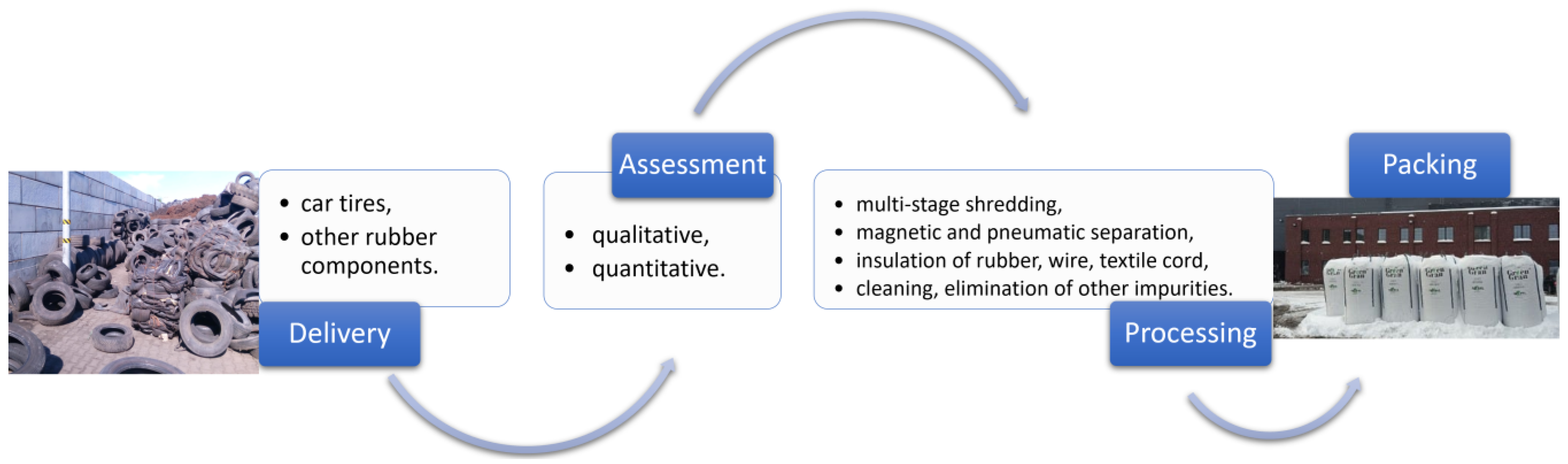
At each of the stages of separation and cleaning of rubber, steel cord, and textile cord in the technological process, waste is generated in the form of low-quality rubber and other solid impurities derived from processing. The waste is an excellent quality alternative fuel that is processed in the combustion process in the cement plant. The general overview of the process is presented in
Figure 2.
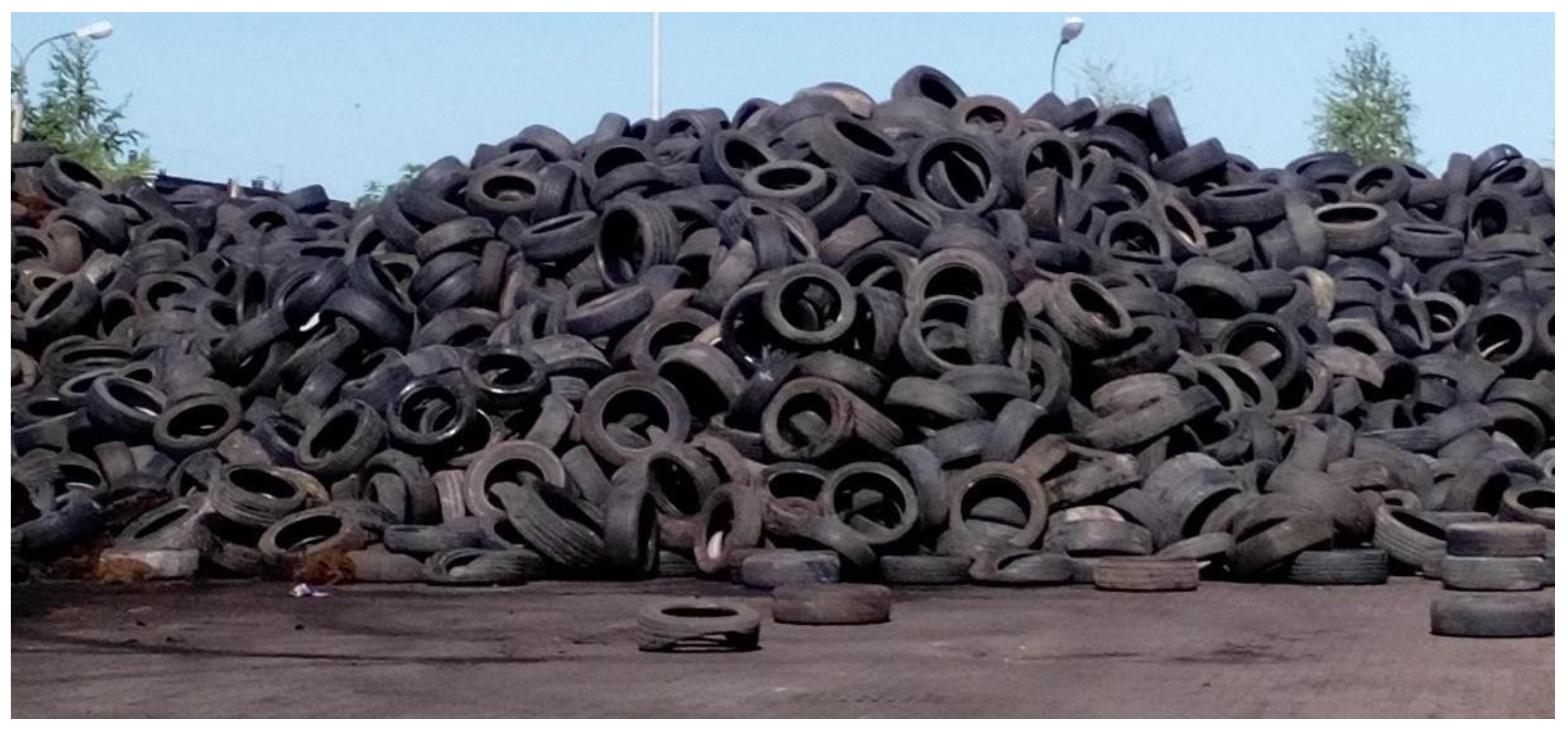
The company processes a total of approx. 47,000 tons of waste per year, including used tires as well as plastics and rubber. In connection to the functioning of the installation, the waste in the form of ferrous metals and alternative fuels is generated. Both types of finished products, i.e., rubber granulate and a stabilizing additive for mineral–asphalt mixes, are widely used in the manufacturing of products, e.g., car mats, slabs and rubber paving stones for playgrounds, etc. Tires are stored in special boxes outside (
Figure 3).
The functioning of this type of company requires a lot of staff involvement and the possession of a modern technological line. The energy potential of waste varies and requires a proper selection and segregation. Therefore, a properly planned, organized and conducted observation of the delivered waste is crucial. The model proposed in the article can successfully support the supply logistics management processes in the surveyed company.
4. Materials and Methods
4.1. Markov Chains
Below, we assume the following: —the set of all real numbers; —a set of natural numbers including zero; —probabilistic space.
Definition 1. A stochastic processis a family of random variablesdefined on the probabilistic spacefor anyandis the set of realizations.
Definition 2. A stochastic processis a Markov process [1,35] if for every, for any finite subset, where,, and for any states,,the propertyis satisfied. Definition 3. A stochastic process is called a homogeneous process [35] if for any,xthe propertyis satisfied. The condition (1.1) is called the Markov property. In the paper, we assume that the set of moments in which we observe the realizations of the stochastic process is a subset of the set of natural numbers, , while the set of realizations of random variables , is a finite set , . The set is called the set of states of the stochastic process. A Markov process with discrete time is called a Markov chain.
Definition 4. A sequence of random variableswith the values in the set of statesis called a Markov chain if, and only if, for anyand,the property [10,39]is satisfied. For a homogeneous Markov chain
, the distribution of transition probabilities between the states is determined by the transition probability matrix
where
for
and
for
, and
is the probability of transition from state
at time
to state
at time
for any
.
For a homogeneous Markov chain, the probability matrix for
steps is
where
is the probability of transition from state
at time
to state
at time
for any
and
for
. Equation (6) is called the Chapman–Kolmogorov equation [
1,
39,
40].
Let , for be the initial distribution for a homogeneous Markov chain with a one-step transition matrix equal to and .
Definition 5. The initial distributionof a homogeneous Markov chainwith transition matrixis stationary if the conditionis satisfied. A homogeneous Markov chain with a stationary initial distribution is called a stationary Markov chain [
1,
39,
40].
4.2. Hidden Markov Models
Hidden Markov model (HMM) is a model consisting of two parts (elements, “layers”): hidden and observed (inner and outer) [
11,
40,
41,
42]. The hidden (inner) part is subordinated to the Markov process, of which the states are not observed (that is why they are called hidden), while we observe the external part of the model where the observed values depend on the realization of the hidden part. The identification of hidden states and the relationship between the hidden and the observed part consists in the analysis of a sequence of events (sequence of states) that has been recorded (observed).
Below, we consider a hidden Markov model with discrete outputs and assume that the hidden part is described by a homogeneous Markov chain:
a set of hidden states;
a set of outputs (set of observed states);
initial distribution, where ;
transition probability matrix between the hidden states, where for any the value denotes the probability of transition from state at time to state at time ;
output probability matrix, where for any quantity is the probability of observing the state at time , provided that the hidden part of the system is in the state .
The elements of the transition matrix and output probability matrix satisfy the condition
and the initial distribution
satisfies the condition
The hidden Markov model with discrete outputs is identified by the set
, where
,
and
, satisfying the conditions (8) and (9) [
6,
40,
41].
4.3. The problem of Identifying Hidden Markov Models
The identification of hidden Markov models consists in estimating the parameters of the model, namely the initial distribution
, the transition probability matrix between the hidden states
and the output probability matrix
, based on the observations
, for
,
. Determination of the structure of HMM
consists in solving three problems [
8,
40].
Problem 1. Estimation of the probability of the sequence of realizationsfor the hidden model of the Markov model, which is the sum of all possible probabilities for the sequences of hidden states,for.
Problem 2. Determination of the sequence of hidden states(Viterbi path), which is best explained for the sequence of observations, whereandfor. Determining the sequencefor the hidden model of the Markov modelconsists in solving the problem Problem 3. Determination of the parametersfor the hidden Markov model consists in solving the problem We use the forward–backward algorithm to estimate the values defined by Equation (10). We use the Viterbi algorithm to determine the sequence of hidden states with the highest probability (11). The values
are determined by maximizing the probability (12) of the occurrence of the series of observations
using the Baum–Welch algorithm [
6,
40,
41].
5. Hidden Markov Models in Forecasting the Supply Sequence
The works [
43,
44] underline that the effective planning of the supply process is the key importance in a company. For the presented company, the assessment of the probable level of supply in the production raw material (i.e., used tires) was analyzed. The company has many suppliers, which is why the tires come from many different sources, and due to the specificity of the assortment, it is often difficult to determine the expected weight of the delivery. The figure below, presenting the level of deliveries over almost three years (
Figure 4), clearly shows how significantly they can vary.
The acceptance of this type of assortment requires the preparation of an appropriate storage place, securing the right number of people and means of transport. In addition, the knowledge of expected deliveries is crucial in planning production processes. Forecasting future deliveries was preceded by an analysis of historical data. First, the deliveries were divided into four types, depending on their weight. This way, the observed states, presented in
Table 1, were distinguished.
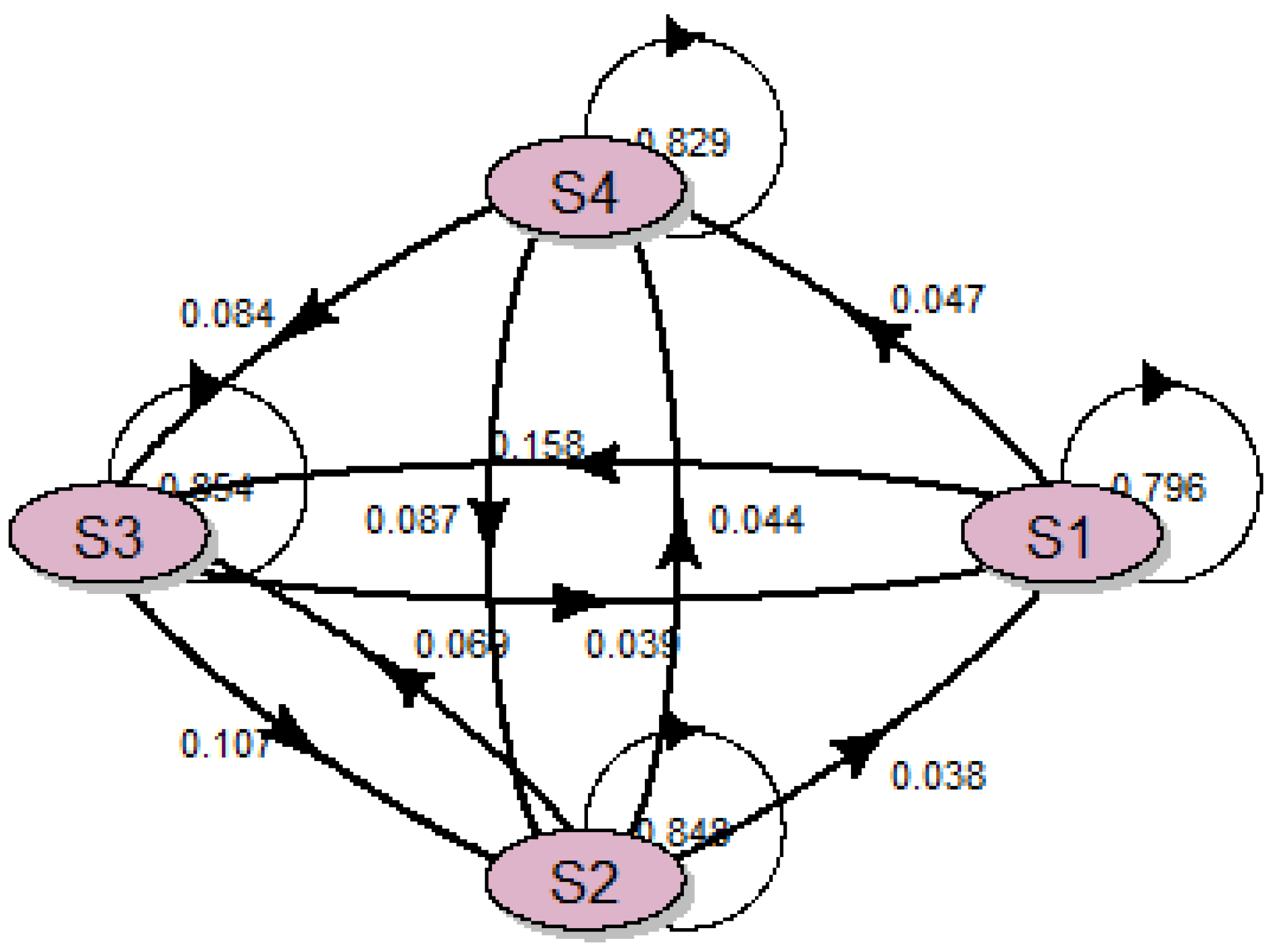
Next, the four hidden states describing the dynamics of the hidden part of the system and using the Markov model for this purpose were determined. In order to describe the dynamics of hidden states, the probability matrix of transitions between the states was determined. These values are presented in the graph showing the relationships between hidden states (
Figure 5).
The above figure shows that the highest values of transitions are for returns to the same state. The values of interstate transitions are much lower. The responses in the form of probabilities of transitions from the hidden states to the observed states are presented in
Table 2.
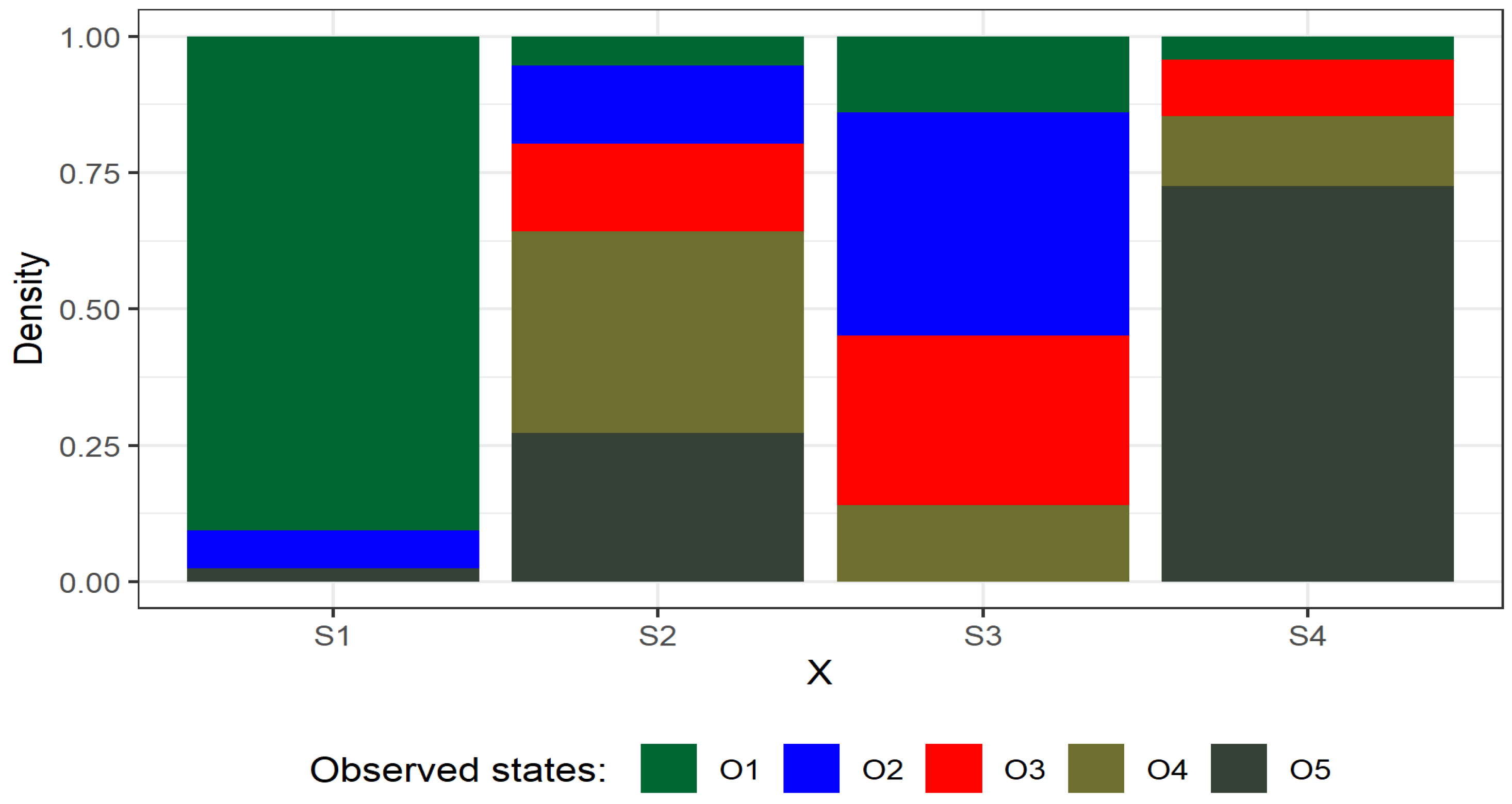
Depending on the relations in the hidden layer, one can infer the probability of the size of the next delivery. Probability distributions of exits from the hidden states to the states observed are shown in a graphical form in
Figure 6.
The description of the model with the use of
Figure 4 and
Figure 5 provides an overview of the behavior of raw material supplies in the supply chain. The probability that a given observed state will occur varies greatly depending on the hidden state. The highest probability values were obtained for the exit from the state S1 to O1 and from S4 to O5. In the event of the hidden state S1, a small supply of raw material (O1) will occur with high probability, while in the case of the hidden state S4 there will be a very large delivery of more than 50 tons.
6. Conclusions
In the article, the authors proposed a description of the supply of raw material to the enterprise using hidden Markov models, different from the time series models, and presented its implementation on the example of a manufacturing enterprise. Observing the order of deliveries, the sequence of the most probable hidden states was identified, the occurrence of which depends only on the state at the moment before. Then, the probabilities of exit from hidden states to the observed states were estimated. This made it possible to forecast the level of supply of raw material for production using hidden Markov models and thus provide the company with the valuable information (with a certain probability) which allows to prepare for the subsequent batches of goods. By identifying the hidden Markov model, we can define and predict changes in the transport schedule. As a result, this will reduce the number of journeys (number of transports), and thus reduce the costs of transporting waste. In addition, reducing the number of transports will have an impact on reducing emissions of harmful substances into the environment.
Additionally, the information obtained from the model allows for better scheduling of work and an even allocation of tasks between employees. If the workload is greater, it is possible to provide proportional salary as well as higher social benefits. Moreover, knowledge of planned deliveries also allows to shape the level of work safety, adjust the necessary equipment and equipment of employees adequately to the type of activities performed and the goods/assortment received.
The presented model is easy to apply directly in the analyzed enterprise. Moreover, the developed method is applicable especially in case of the observed features, phenomena or systems that are characterized by rapid changes, discontinuity or significant seasonality. It is the response to the volatility of the market and its randomness as well as a tool for forecasting that counteracts the negative impact of external factors on the quality of forecasting.
The next step of the research will be the development of models using other methods as well as the comparison and evaluation of the obtained results.
Author Contributions
Conceptualization, A.B. and E.K.; methodology, A.B. and E.K.; software, E.K.; validation A.B. and E.K.; formal analysis, A.B. and E.K.; investigation, A.B. and E.K.; resources, R.P., L.G. and D.P.; data curation, R.P.; writing—original draft preparation, A.B., E.K., L.G. and D.P.; writing—review and editing, A.B., E.K., L.G., K.A. and D.P.; visualization, A.B., R.P. and E.K.; supervision, A.B. and K.A.; project administration, A.B. and K.A.; funding acquisition, K.A. All authors have read and agreed to the published version of the manuscript.
Funding
This research received no external funding.
Institutional Review Board Statement
Not applicable.
Informed Consent Statement
Not applicable.
Data Availability Statement
Not applicable.
Conflicts of Interest
The authors declare no conflict of interest.
References
- Baum, L.E.; Petrie, T. Statistical inference for probabilistic functions of finite state markov chains. Ann. Math. Stat. 1966, 37, 1554–1563. [Google Scholar] [CrossRef]
- Zhang, M.; Chen, X.; Li, W. A Hybrid Hidden Markov Model for Pipeline Leakage Detection. Appl. Sci. 2021, 11, 3138. [Google Scholar] [CrossRef]
- Martins, A.; Fonseca, I.; Farinha, J.T.; Reis, J.; Cardoso, A.J.M. Maintenance Prediction through Sensing Using Hidden Markov Models—A Case Study. Appl. Sci. 2021, 11, 7685. [Google Scholar] [CrossRef]
- Mor, B.; Garhwal, S.; Kumar, A. A systematic review of hidden Markov models and their applications. Arch. Comput. Methods Eng. 2021, 28, 1429–1448. [Google Scholar] [CrossRef]
- Alghamdi, R. Hidden Markov models (HMMs) and security applications. Int. J. Adv. Comput. Sci. Appl. 2016, 7, 39–47. [Google Scholar] [CrossRef] [Green Version]
- Robles, B.; Avila, M.; Duculty, F.; Vrignat, P.; Begot, S.; Kratz, F. Methods to choose the best Hidden Markov Model topology for improving maintenance policy. In Proceedings of the 9th International Conference on Modeling, Optimization & SIMulation, Boredaux, France, 6–8 June 2012. [Google Scholar]
- Nguyen-Le, D.H.; Tao, Q.B.; Nguyen, V.H.; Abdel-Wahab, M.; Nguyen-Xuan, H. A data-driven approach based on long short-term memory and hidden Markov model for crack propagation prediction. Eng. Frac. Mech. 2020, 235, 107085. [Google Scholar] [CrossRef]
- Malhotra, R.; Singla, C.; Farooque, D. Comparison of Hidden Markov Model with other Machine Learning Techniques in Software Defect Prediction. In Proceedings of the 2022 IEEE 7th International Conference for Convergence in Technology (I2CT), Mumbai, India, 7–9 April 2022; pp. 1–5. [Google Scholar]
- Borucka, A. Logistic regression in modeling and assessment of transport services. Open Eng. 2020, 10, 26–34. [Google Scholar] [CrossRef] [Green Version]
- Oszczypała, M.; Ziółkowski, J.; Małachowski, J. Analysis of Light Utility Vehicle Readiness in Military Transportation Systems Using Markov and Semi-Markov Processes. Energies 2022, 15, 5062. [Google Scholar] [CrossRef]
- Ziółkowski, J.; Małachowski, J.; Oszczypała, M.; Szkutnik-Rogoż, J.; Konwerski, J. Simulation model for analysis and evaluation of selected measures of the helicopter’s readiness. Proc. Inst. Mech. Eng. Part G J. Aerosp. Eng. 2022, 236, 2751–2762. [Google Scholar] [CrossRef]
- Hsieh, M.C.; Giloni, A.; Hurvich, C. The propagation and identification of ARMA demand under simple exponential smoothing: Forecasting expertise and information sharing. IMA J. Manag. Math. 2020, 31, 307–344. [Google Scholar] [CrossRef]
- Sulandari, W.; Subanar, S.; Rodrigues, P.C. Exponential smoothing on modeling and forecasting multiple seasonal time series: An overview. Fluct. Noise Lett. 2021, 20, 2130003. [Google Scholar] [CrossRef]
- Lolli, F.; Coruzzolo, A.M.; Peron, M.; Sgarbossa, F. Age-based preventive maintenance with multiple printing options. Int. J. Prod. Econ. 2022, 243, 108339. [Google Scholar] [CrossRef]
- Cantini, A.; Peron, M.; De Carlo, F.; Sgarbossa, F. A decision support system for configuring spare parts supply chains considering different manufacturing technologies. Int. J. Prod. Res. 2022, 60, 1–21. [Google Scholar] [CrossRef]
- Kusuma, N.; Roestam, M.; Pasca, L. The analysis of forecasting demand method of linear exponential smoothing. J. Educ. Adm. Manag. Leadersh. 2021, 1, 7–18. [Google Scholar] [CrossRef]
- Sinaga, H.; Irawati, N. A medical disposable supply demand forecasting by moving average and exponential smoothing method. In Proceedings of the 2nd Workshop on Multidisciplinary and Applications (WMA), Padang, Indonesia, 24–25 January 2018; pp. 24–25. [Google Scholar]
- Rostami-Tabar, B.; Babai, M.Z.; Ali, M.; Boylan, J.E. The impact of temporal aggregation on supply chains with ARMA (1, 1) demand processes. Eur. J. Oper. Res. 2019, 273, 920–932. [Google Scholar] [CrossRef]
- Hofmann, E.; Rutschmann, E. Big data analytics and demand forecasting in supply chains: A conceptual analysis. Int. J. Log. Man. 2018, 29, 739–766. [Google Scholar] [CrossRef]
- Seyedan, M.; Mafakheri, F. redictive big data analytics for supply chain demand forecasting: Methods, applications, and research opportunities. J. Big Data 2020, 7, 53. [Google Scholar] [CrossRef]
- Zvolenský, P.; Barta, D.; Grenčík, J.; Droździel, P.; Kašiar, L. Improved method of processing the output parameters of the diesel locomotive engine for more efficient maintenance. Eksploat. Niezawodn. Maint. Reliab. 2021, 23, 315–323. [Google Scholar] [CrossRef]
- Huang, L.; Xie, G.; Zhao, W.; Gu, Y.; Huang, Y. Regional logistics demand forecasting: A BP neural network approach. Complex Intell. Syst. 2020, 1–16. [Google Scholar] [CrossRef]
- Bandara, K.; Shi, P.; Bergmeir, C.; Hewamalage, H.; Tran, Q.; Seaman, B. Sales demand forecast in e-commerce using a long short-term memory neural network methodology. In Proceedings of the International Conference on Neural Information Processing, Sydney, Australia, 12–15 December 2019; Springer: Cham, Switzerland, 2019; pp. 462–474. [Google Scholar] [CrossRef]
- Aamer, A.; Eka Yani, L.; Alan Priyatna, I. Data analytics in the supply chain management: Review of machine learning applications in demand forecasting. Oper. Supply Chain Manag. 2020, 14, oscm0440281. [Google Scholar] [CrossRef]
- Wen, Z.; Xie, L.; Fan, Q.; Feng, H. Long term electric load forecasting based on TS-type recurrent fuzzy neural network model. Electr. Power Syst. Res. 2020, 179, 106106. [Google Scholar] [CrossRef]
- Jiang, P.; Li, R.; Liu, N.; Gao, Y. A novel composite electricity demand forecasting framework by data processing and optimized support vector machine. Appl. Energy 2020, 260, 114243. [Google Scholar] [CrossRef]
- Güven, İ.; Şimşir, F. Demand forecasting with color parameter in retail apparel industry using artificial neural networks (ANN) and support vector machines (SVM) methods. Comput. Ind. Eng. 2020, 147, 106678. [Google Scholar] [CrossRef]
- Perea, R.G.; Poyato, E.C.; Montesinos, P.; Díaz, J.R. Prediction of irrigation event occurrence at farm level using optimal decision trees. Comput. Electron. Agric. 2019, 157, 173–180. [Google Scholar] [CrossRef]
- Nowakowski, T.; Komorski, P. Diagnostics of the drive shaft bearing based on vibrations in the high-frequency range as a part of the vehicle’s self-diagnostic system. Eksploat. Niezawodn. Maint. Reliab. 2022, 24, 70–79. [Google Scholar] [CrossRef]
- Antosz, K.; Jasiulewicz-Kaczmarek, M.; Paśko, Ł.; Zhang, C.; Wang, S. Application of machine learning and rough set theory in lean maintenance decision support system development. Eksploat. Niezawodn. Maint. Reliab. 2021, 23, 695–708. [Google Scholar] [CrossRef]
- Lin, L.; Guo, H.; Lv, Y.; Liu, J.; Tong, C.; Yang, S. A machine learning method for soil conditioning automated decision-making of EPBM: Hybrid GBDT and Random Forest Algorithm. Eksploat. Niezawodn. Maint. Reliab. 2022, 24, 237–247. [Google Scholar] [CrossRef]
- Punia, S.; Nikolopoulos, K.; Singh, S.P.; Madaan, J.K.; Litsiou, K. Deep learning with long short-term memory networks and random forests for demand forecasting in multi-channel retail. Int. J. Prod. Res. 2020, 58, 4964–4979. [Google Scholar] [CrossRef]
- Dhanalakshmi, J.; Ayyanathan, N. An implementation of energy demand forecast using J48 and simple K means. In Proceedings of the 2019 Fifth International Conference on Science Technology Engineering and Mathematics (ICONSTEM), Chennai, India, 14–15 March 2019; IEEE: Piscataway, NJ, USA, 2019; Volume 1, pp. 174–178. [Google Scholar] [CrossRef]
- Huber, J.; Stuckenschmidt, H. Daily retail demand forecasting using machine learning with emphasis on calendric special days. Int. J. Forecast. 2020, 36, 1420–1438. [Google Scholar] [CrossRef]
- Al-Musaylh, M.S.; Deo, R.C.; Adamowski, J.F.; Li, Y. Short-term electricity demand forecasting using machine learning methods enriched with ground-based climate and ECMWF Reanalysis atmospheric predictors in southeast Queensland, Australia. Renew. Sustain. Energy Rev. 2019, 113, 109293. [Google Scholar] [CrossRef]
- Racewicz, S.; Kutt, F.; Sienkiewicz, Ł. Power Hardware-In-the-Loop Approach for Autonomous Power Generation System Analysis. Energies 2022, 15, 1720. [Google Scholar] [CrossRef]
- Projekt Budowlany. Mirosław Stachowski; RECYKL Organizacja Odzysku S.A, Projektowe Usługi Budowlane: Rawicz, Poland, 2019. (In Polish) [Google Scholar]
- Rajca, P.; Zajemska, M. Ocena możliwości paliwa RDF na cele energetyczne. Rynek Energii 2018, 4, 137. (In Polish) [Google Scholar]
- Privault, N. Understanding Markov Chains; Springer: Singapore, 2018. [Google Scholar] [CrossRef]
- Mamon, R.S.; Elliott, R.J. (Eds.) Hidden Markov Models in Finance; Springer US: Newy York, NY, USA, 2007. [Google Scholar] [CrossRef]
- Zucchini, W.; MacDonald, I.L.; Langrock, R. Hidden Markov Models for Time Series, Chapman; Hall/CRC: Boca Raton, FL, USA, 2017. [Google Scholar] [CrossRef]
- Rabiner, L.R. A tutorial on hidden markov models and selected applications in speech recognition. Proc. IEEE. 1989, 77, 257–286. [Google Scholar] [CrossRef] [Green Version]
- Giri, B.C.; Glock, C.H. The bullwhip effect in a manufacturing/remanufacturing supply chain under a price-induced non-standard ARMA (1,1) demand process. Eur. J. Oper. Res. 2022, 301, 458–472. [Google Scholar] [CrossRef]
- Wang, Z. Intelligent Value-Added System Service of Automobile Manufacturing Enterprise Based on Forecast Demand Algorithm Analysis. In Proceedings of the International Conference on Big Data Analytics for Cyber-Physical-Systems, Shanghai, China, 28 November 2021; Springer: Singapore, 2021; pp. 1047–1055. [Google Scholar] [CrossRef]
| Disclaimer/Publisher’s Note: The statements, opinions and data contained in all publications are solely those of the individual author(s) and contributor(s) and not of MDPI and/or the editor(s). MDPI and/or the editor(s) disclaim responsibility for any injury to people or property resulting from any ideas, methods, instructions or products referred to in the content. |
© 2022 by the authors. Licensee MDPI, Basel, Switzerland. This article is an open access article distributed under the terms and conditions of the Creative Commons Attribution (CC BY) license (https://creativecommons.org/licenses/by/4.0/).

 ,
, 


