Research on the Landslide Prediction Based on the Dual Mutual-Inductance Deep Displacement 3D Measuring Sensor

Featured Application

Based on a novel multi-sensor system for monitoring the deep displacement of slopes, the feasibility of previous work was verified. A new multivariate gray model was developed to predict displacement values with more accurate results than some previous methods. A new discriminative method for slope stability is proposed which can be used to determine hazards in advance, avoiding the vulnerability of previous methods to environmental influences.

Abstract

Landslides are frequent and catastrophic geological hazards, and forecasting their movement is an important aspect of risk assessment and engineering prevention. Based on the integrated deep displacement three-dimensional measuring sensor with sensing unit array structure, an improved multivariable grey model based on dynamic background value and multivariable feedback is proposed to build predictive models for the evolutionary condition of landslides. In the modeling process, the traditional grey model was replaced by extracting the trend information of each variable, instead of summing up each independent variable after assigning weights to it, besides, the Whale Optimization Algorithm (WOA) is used to modify the default value in the model’s background variables. By predicting more than 1000 sets of deep displacement monitoring data collected in the landslide simulation test conducted at the landslide simulation test device, the displacement prediction accuracy of our purposed model is 26%, 47%, and 87% respectively higher than the optimizing grey model (OGM) for three sensing units at different depths. Moreover, a new landslide risk assessment approach based on the orientation vector angle is proposed to make stability discriminations which is less susceptible to volatile data than the TOPSIS-Entropy weight theory and avoids the problem of lack of uniform standards due to the complexity of environmental factors.

1. Introduction

A landslide is a kind of global natural disaster that is mainly caused by rainfall, earthquake, and human activities that can lead to huge damage to infrastructure and the economy even the loss of life [1]. For example, the Shuicheng landslide that happened in China in July 2019 caused 42 deaths and 9 missing people [2]. Likewise, the Kavalappara landslide that happened in India in 2019 caused 46 deaths and 11 missings [3]. There are many parameters to monitor landslides such as displacement, soil stress, hydrology, and precipitation [4]. Among them, displacement is currently one of the most dominant and commonly used parameters of geological hazard monitoring. Displacement monitoring can be divided into surface displacement and deep displacement monitoring, especially the latter provides accurate information for determining the location of sliding surfaces and assessing the states of landslides [5]. Additionally, the predictive techniques for the landslide are essential to reinforce slopes earlier to prevent disasters or to help emergency response systems gain more time to organize evacuations.

Many instruments and techniques have been used to monitor the slope surface displacement, including GPS technology [6,7,8], geodetic method [9,10,11,12], and Interferometric Synthetic Aperture Radar technology [13,14,15], etc. At present, surface displacement monitoring technology has been developed to a relatively high level, which generally has the characteristics of stable performance, high precision, automatic real-time monitoring and so on. However, since the surface displacement monitoring cannot reflect the deformation characteristics of the deep rock and soil mass, it does not meet the needs of stability analysis and management engineering design in many cases. For example, GPS technology can only monitor the displacement or settlement of the site where the sensor is located, and the measurement accuracy is vulnerable to weather [16,17], meanwhile, the Interferometric Synthetic Aperture Radar technology is difficult to monitor the landslide displacement covered with luxuriant trees and needs unmanned aerial vehicles (UAVs) to assist, which is complex to operate and cannot be monitored in real-time [18].

Compared with the surface displacement monitoring technology, the complexity of the monitoring environment leads to slower development of deep displacement monitoring technology. The borehole inclinometer is the most widely used technology, which has been proven capable of monitoring the occurrence of landslides in advance [19,20]. However, it is low-efficiency because manual reading is required for each measurement, worse yet, along with the continuous evolution of the landslide deformation, the inclinometer tube in the borehole is vulnerable to being broken or extruded, which will make the sliding inclinometer unable to sink into the borehole for further measurement. Time-domain reflectometry [21,22,23] is another remote electronic measurement technology that can be used to monitor the displacement but this method cannot determine the direction of landslide movement, nor can it be used in rock and soil mass without shear force. With the development of technology, a new type of displacement monitoring instrument, Fiber Bragg Grating technology [24,25], has been developed. Even though this technology has the features of anti-electromagnetic interference, long transmission distance, it is sensitive to temperature and easy to break during large deformations [26].

When sufficient monitoring data are obtained, various mathematical methods can be used to predict the landslide displacement relatively accurately. These methods can be classified into two categories. The first one is the model-driven prediction methods [27,28], mainly based on geographic and geomorphic conditions and general creep theories. However, such methods are usually complex and have many limitations. On the one hand, they can only be used for these landslides that have occurred, and the final states are necessary to be known so as to calculate the intermediate process of disasters. On the other hand, each model can only be used for a specific process, which lacks robustness.

The other is the data-driven prediction model method on the basis of historical data, which is more widely used in engineering practice. It does not need to take too many geographical factors into account that it can be widely used in different cases. Various methods were developed in previous research, such as the information value model [29,30,31,32], regression model [33,34], grey model [35,36,37,38], random forests [39,40,41], and artificial neural network [42,43,44]. These methods can be divided into small-sample methods and large-sample methods based on the sample size. The large sample method is often more widely used. In addition to displacement monitoring data, large sample methods usually require monitoring data such as precipitation, soil moisture, water level, etc. Machine learning is a typical representation of the large sample method. It can consider the nonlinear behaviors and correlations in the historical monitoring data of different variables. However, in complex field monitoring scenarios, due to the failure of monitoring instruments or human factors, the actual landslide monitoring data may have large noise and data loss, resulting in inaccurate prediction results. Small sample prediction is often used for data samples with stable, exponential, and convergent characteristics, and the grey model is the most common mathematical model in small sample landslide prediction. Under the same sample size, the computational complexity of the grey model is significantly smaller than that of artificial neural networks, extreme learning machines, and deep learning machines. Since landslides are non-integral movements in most cases, the displacement usually first appears in the interior of the rock and soil mass and gradually passes upward to the surface, so it is more practical to evaluate the stability and early forecast of landslides through deep displacement monitoring.

In order to overcome these questions mentioned above, in previous work, a new deep displacement measuring sensor based on dual mutual inductance [45] has been developed. The whole sensor adopts a sensing array structure, thus, the sensor can deform synchronously with the surrounding rock and soil mass, and the distance and direction of the sensing unit are approximately equal to the displacement of the surrounding rock and soil mass. Each sensing unit contains an air-core coil, a magnetic-core coil, associated circuitry, and software. It has the advantage of flexible structure design, automatic measurement, and high measurement accuracy. More importantly, it can reflect the three-dimensional displacement change of deep displacement of rock and soil mass.

In this work, due to the long collection time of the entire sensor, it is impossible to use large sample methods to predict. Therefore, an improved grey model to predict the displacement of landslides and a new method to determine the stability of slopes are proposed, so as to make full use of the monitoring data from the new deep displacement monitor sensor. As this sensor is still in the testing stage, it is not suitable to apply it to the field. Thus, we have built a landslide simulation experiment platform to simulate the landslide occurrence process, so as to check the monitoring performance of the entire sensor. The sequence of the article can be summarized as follows. The platform of the landslides simulation experiment and the integrated deep displacement three-dimensional measuring sensor are described in Section 2. The definition of the original grey model, the improved grey model, and the new method for landslide stability discrimination are introduced in Section 3. The experimental process and results are presented in Section 4 and the conclusions are in Section 5.

2. Landslide Experiment Equipment

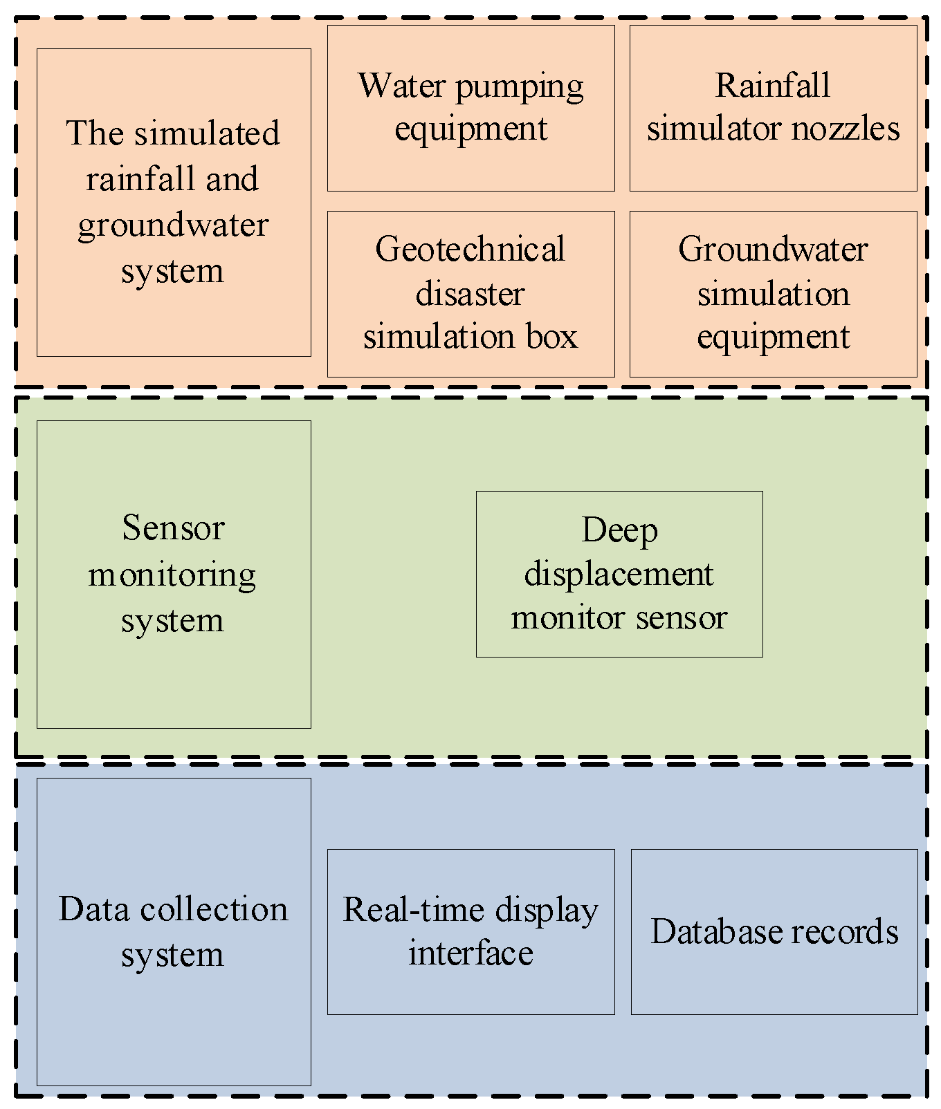
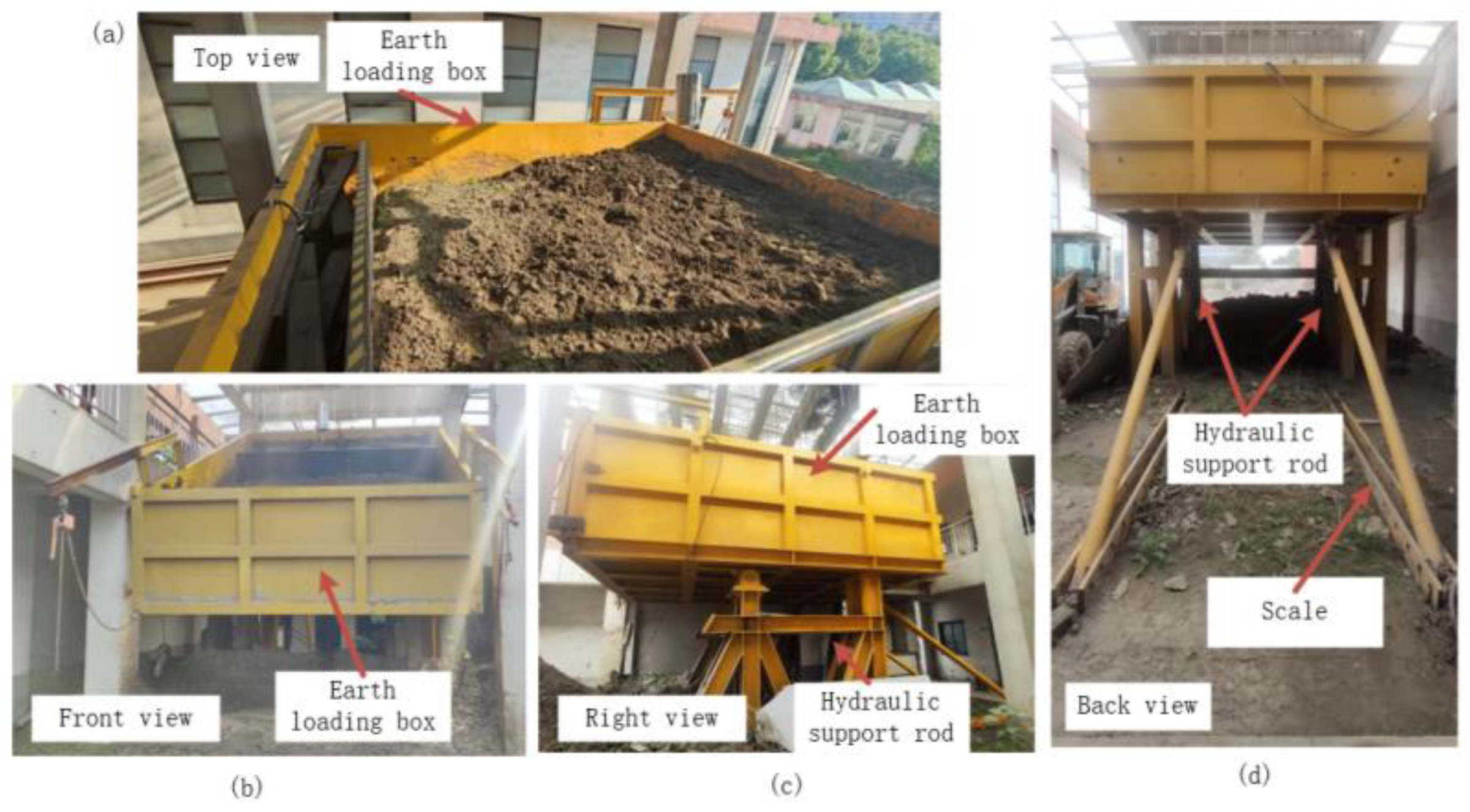
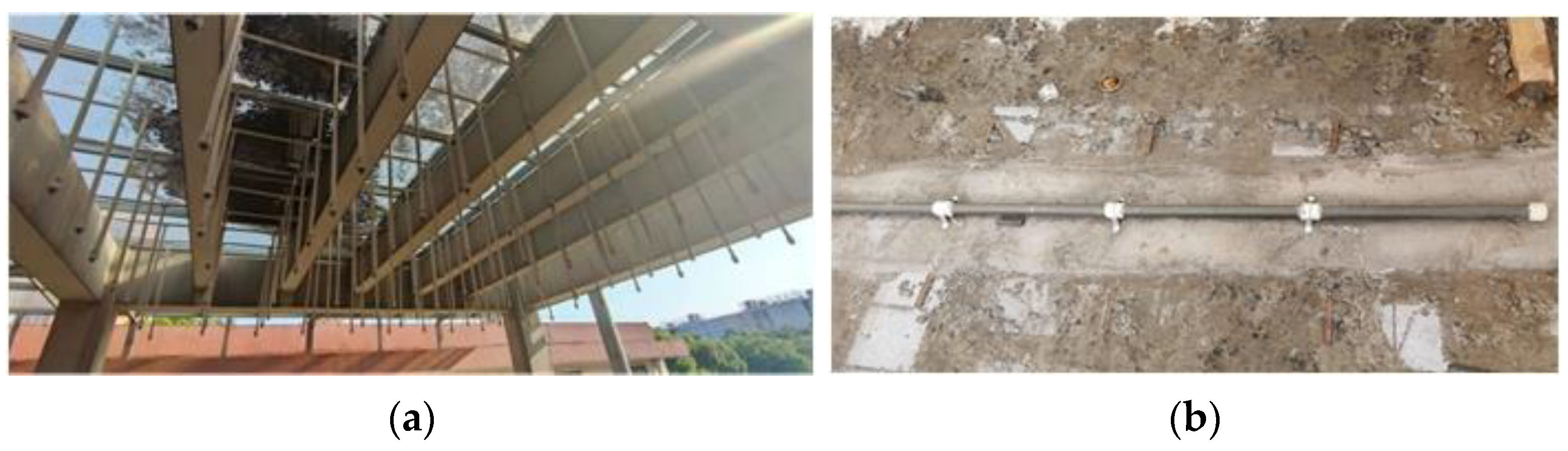
2.1. Experiment Platform

In order to simulate the process of landslide, an artificial landslide simulation experiment device was designed. The whole device consists of three parts (Figure 1), the simulated rainfall and the groundwater system, the sensor monitoring system, and the data collection system.

As is shown in Figure 2, the geotechnical disaster simulator box is lifted by hydraulic support rods and the door of the earth loading box can open by gravity. Thus, it will not hinder the displacement of landslide soil. The gradient of the slope can be adjusted freely from 0 to 60 degrees to simulate the different actual conditions. Figure 2a is the top view of the simulator box. When the experiment starts, the box will be full of rock and soil. Figure 2b is the front view where the door of the earth loading box, the angle of the door will gradually increase with the tilt of the whole box. Figure 2c,d is the right view and back view of the equipment respectively. As is shown in the picture, the box is lifted by hydraulic support rods and the gradient of the slope can be observed by the scale.

It is shown in Figure 3 that the rainfall system consists of 10 rows and 10 columns of rainfall nozzles and the groundwater system consist of a 4-m-long porous ceramic tube that can slowly leak water and will not be clogged with dirt. In this way, the groundwater levels can be more realistically imitated.

As shown in Figure 4, the new deep displacement monitor sensor uses several identical sensing units for the deep displacement measurements of slopes. The relative displacement between each adjacent unit is measured at first, and then the whole deep displacement can be calculated by accumulation, the new deep displacement monitor sensor takes about two minutes to complete displacement data acquisition each time. The principle of the sensor will be expounded in the next subsection.

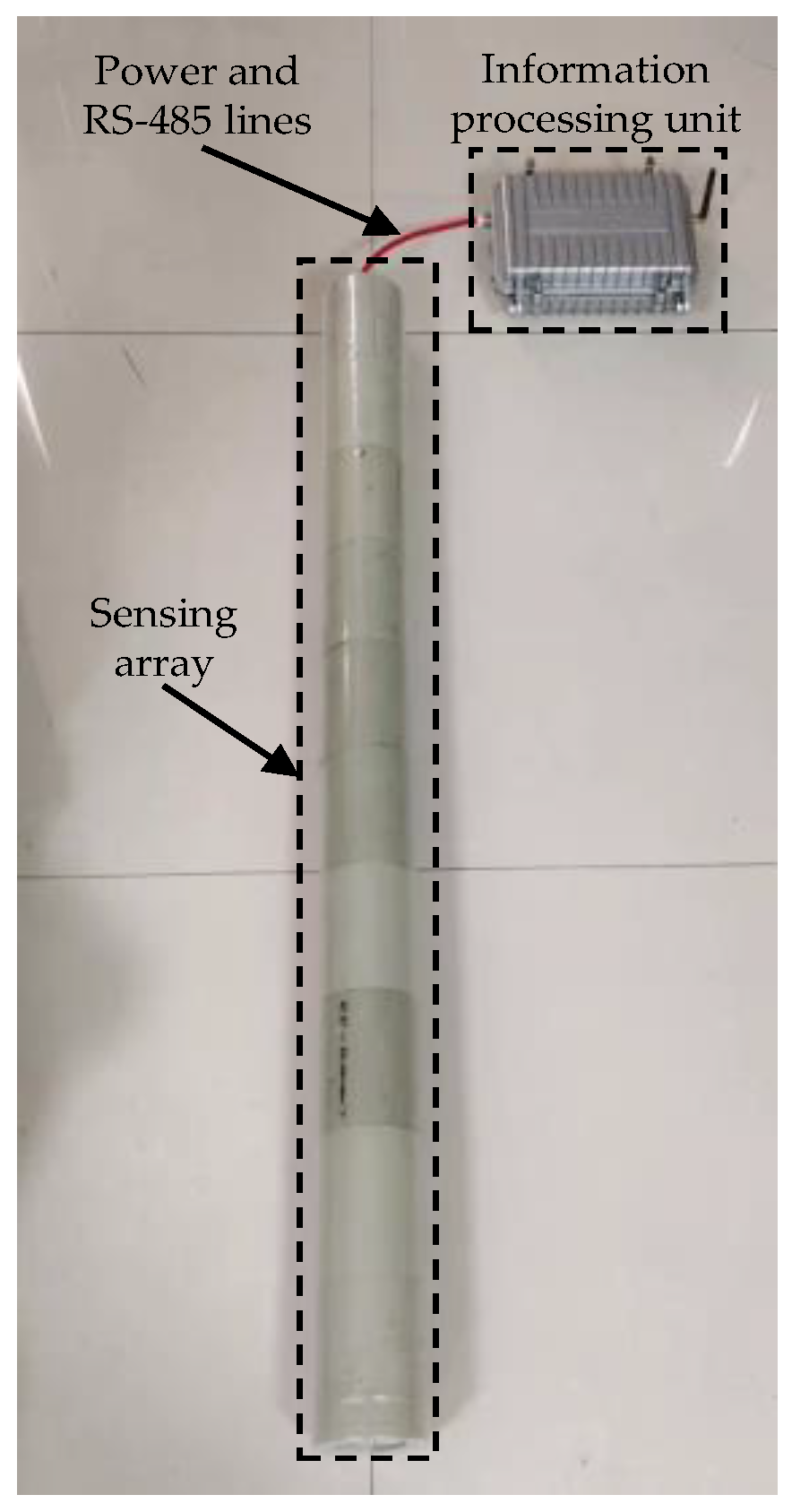
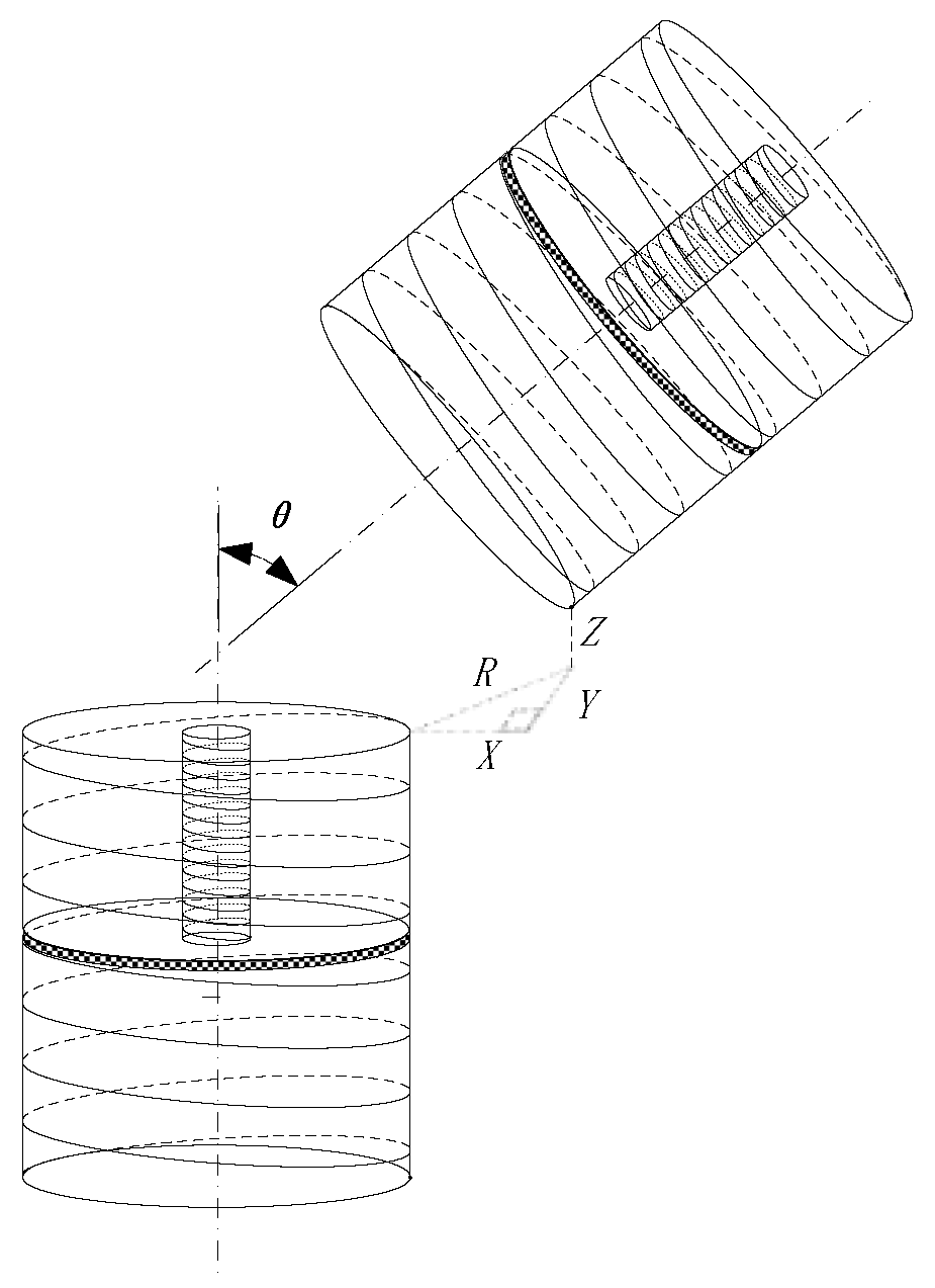
2.2. Introduction to the Principle of Deep Displacement Monitor Sensor

The principle of the deep displacement monitor sensor based on the double mutual inductance voltage contour method is shown in Figure 5. The whole instrument is composed of several identical sensing units. Each sensing unit is 10 cm high, and the number of sensors in a sensing array is determined by the depth of the bedrock. Each sensing unit consists of an external air-core coil, an internal coil with a magnetic core, associated circuitry, and structure. The lower sensing unit is referred to as the excitation end while the upper sensing unit is called the measurement end. The upper and lower sensing units form a group of measuring units. Therefore, N sensing units form N − 1 measuring units from bottom to top. When the air-core coil and the core coil at the excitation end are connected to the same sinusoidal signal, due to the electromagnetic induction, two mutual inductance voltages with the same frequency and different amplitude will be generated on the air-core coil at the measurement end.

Since the sensing array is located in the same environment and each unit has the same structure, the mutual voltage is only related to the relative tilt angle and position between adjacent sensing units. Therefore, when any of the horizontal resultant displacement R, vertical displacement Z and tilt angle θ in Figure 5 change, the mutual inductance voltage collected in the measuring unit will change. Since any vector on the XOY plane consists of two components, the horizontal resultant displacement can be divided into two vectors, X and Y.

For any two adjacent sensing units, the measurement model for describing the relationship between the relative displacement and the double mutual inductance voltage can be established by the following methods. (1) Collecting the data of the mutual inductance voltage at different relative inclination angles θ, horizontal displacement R, and vertical displacement Z. (2) Quantify this data by theoretical analysis and experimental testing. (3) Using the model established in step 2, the change of the relative position between adjacent sensing units can be calculated by collecting the change of the double mutual inductance voltage.

3. Methodology

3.1. Prediction Model

Since the deep displacement monitor sensor consists of several identical sensing units, there is a strong correlation among the units, so the multivariate grey prediction model is more effective than the univariate grey prediction model in predicting the displacement of landslides. The traditional GM(1, N) model [46] is often used to analyze the influences of several influencing factors on the system behavior variables. Here is the definition of it. Assuming that X₁⁽⁰⁾ is the system characteristic sequence while the X_i⁽⁰⁾(i = 2, 3, …, N) is the series of explanatory variables having high correlations with sequence X₁⁽⁰⁾.

$$\begin{array}{c}{X}_1^{(0)}=(x_1^{(0)}(1),x_1^{(0)}(2),\dots ,x_1^{(0)}(m))\\ X_2^{(0)}=(x_2^{(0)}(1),x_2^{(0)}(2),\dots ,x_2^{(0)}(m))\\ ⋮\\ X_{\mathrm{N}}^{(0)}=(x_{\mathrm{N}}^{(0)}(1),x_{\mathrm{N}}^{(0)}(2),\dots ,x_{\mathrm{N}}^{(0)}(m))\end{array}$$

(1)

The first-order accumulative generation operation (1-AGO), defined as Equation (2), generates the first-order cumulative sequence X_j⁽¹⁾(j = 1, 2, …, N).

$$\begin{array}{l}{X}_j^{(0)}=(x_j^{(0)}(1),x_j^{(0)}(2),\dots ,x_j^{(0)}(m))\\ x_j^{(0)}(k)={\displaystyle {\sum }_{g=1}^k{x}_j^{(0)}(g)},k=1,2,\dots ,m\end{array}$$

(2)

Z₁⁽¹⁾ is the sequence of immediately adjacent mean generation of X₁⁽¹⁾, defined as follows.

$$\begin{array}{l}{Z}_1^{(1)}=(z_1^{(1)}(2),z_1^{(1)}(3),\dots ,z_1^{(1)}(m))\\ z_1^{(1)}(k)=0.5\times (x_1^{(1)}(k)+x_1^{(1)}(k-1)),k=2,3,\dots ,m\end{array}$$

(3)

Then Equation (4) is the discrete grey model with multiple variables where a and b_i can be calculated by least-squares estimation.

$$x_1^{(0)}(k)+a{z}_1^{(1)}(k)={\displaystyle {\sum }_{i=2}^N{b}_i{x}_1^{(1)}(k)}$$

(4)

According to previous research, the GM(1, N) model has some serious flaws. First, the GM(1, N) model is a first-order grey system prediction model with N variables, however, when N equals 1, this model cannot be converted to GM(1, 1) model equivalently. Second, the final expression is derived by an ideal simplification method, which may make a mismatch with the actual situation [47]. Finally, the default background value of 0.5 is used in the adjacent mean generation, resulting in large errors in fitting and prediction. Tan [48] had proposed an improved background value method to compensate for this flaw.

Yang proposed an optimizing grey model [49] to solve part of the first and second drawbacks mentioned above. Let X₁⁽⁰⁾ be the system behavior characteristic’s original non-negative sequence.

$$X_1^{(0)}=(x_1^{(0)}(1),x_1^{(0)}(2),\dots ,x_1^{(0)}(m))$$

(5)

X_i⁽⁰⁾(i = 2, 3, …, N) are the original positive sequence containing N − 1 related factors, X_j⁽¹⁾ is the 1-AGO sequence of X_j⁽⁰⁾(j = 1, 2, …, N) and Z₁⁽¹⁾ is the sequence of immediately adjacent mean generation of X₁⁽¹⁾

$$\begin{array}{l}{X}_i^{(0)}=(x_i^{(0)}(1),x_i^{(0)}(2),\dots ,x_i^{(0)}(m))\\ X_j^{(1)}=(x_j^{(1)}(1),x_j^{(1)}(2),\dots ,x_j^{(1)}(m))\\ Z_1^{(1)}=(z_1^{(1)}(1),z_1^{(1)}(2),\dots ,z_1^{(1)}(m))\end{array}$$

(6)

The linear correction term h₁(k − 1) and the grey action h₂ are shown in the following model, which is the first-order differential optimizing grey model with N variables, abbreviated as OGM(1, N).

$${\mathrm{x}}_i^{(0)}(k)+a{z}_1^{(1)}(k)={\displaystyle {\sum }_{i=2}^N{b}_i{x}_i^{(1)}(k)+h_1(k-1)+}{h}_2$$

(7)

Based on the previous research and combined with the research object of this article, a further optimization of the grey model has been made.

A system often consists of several interrelated factors, and the development trend of the system behavior factor is fed by the other influencing variables in the system. In the control feedback process of the traditional multivariate discrete grey prediction model, the system development parameters are often set in constant coefficients, and may deviate from the actual situation.

The actual system developmental dynamics parameters are often multivariate influenced and time-varying. First, the developmental dynamics are not only related to the development of the system itself but are also affected by the development dynamics of other influencing factors of the system. Second, the developmental dynamics of the influencing factors make the system’s developmental dynamics constantly change over time.

Considering the above two features, a grey model with the trend information of development factors and a dynamic background-value coefficient has been proposed, or, N-variable Feedback Optimizing Background Grey Model, abbreviated as FOBGM (1, N) for convince.

As shown in Figure 6, AGO is the accumulating generation operator which can reduce the effects of stochastic variation in system behavior factors and their influences by cumulative generation. The ρ, defined in Equation (8), is called an extractor which is used to extract information on the development trend of influencing factors. The γ_i(i = 1, 2, …, m − 1) are named as parameters of developmental states.

$$\rho =\frac{x^{(0)}(t+1)}{x^{(1)}(t)}$$

(8)

Assume that X1(0) and Xj(0) are the same as they were previously defined. Equation (9) is the OGM(1, N) with development factor trend information and a dynamic background value, which is the FOBGM(1, N)

$$(1+a\xi ){\widehat{x}}_1^{(1)}(k)=\beta (1+{\rho }_a(k))x_1^{(1)}(k-1)+(1-a+a\xi )x_1^{(1)}(k-1)+kc+d$$

(9)

where the ξ is the background value ranging from 0 to 1. The ρa is the integrated system development situation, defined in Equation (10).

$${\rho }_a(k)={\gamma }_1\frac{x_2^{(0)}(k)}{x_2^{(1)}(k-1)}+{\gamma }_2\frac{x_3^{(0)}(k)}{x_3^{(1)}(k-1)}+\cdots +{\gamma }_{n-1}\frac{x_n^{(0)}(k)}{x_n^{(1)}(k-1)}$$

(10)

The p₁ and p₂ are the parameter sequences of the new model, as stated in Equation (11). The least-square method may be used to estimate both sequences. Once the p₁ and p₂ have already known, the ξ will take the minimum case of the Mean Absolute Percentage Error (MAPE) between the calculated values and actual series X₁⁽⁰⁾ as its value, establishing the OGM(1, N) model with trend information of development components and a dynamic background-value coefficient.

$$\begin{array}{l}{p}_1=[\beta ,a,c,d]\\ p_2=[{\gamma }_1,{\gamma }_2,\cdots ,{\gamma }_{n-1}]\end{array}$$

(11)

The parameters of FOBGM(1, N) are going to be estimated by ordinary least squares(OLS). Let the X_i⁽⁰⁾(i = 1, 2, …, N) and X_j⁽¹⁾(j = 1, 2, …, N) are defined in Equation (5), and the p₁ can satisfy Equation (12) by least squares estimation.

$$\begin{array}{l}{p}_1={(E^{T}E)}^{-1}{E}^{T}S\\ \end{array}$$

(12)

The E and S are defined as follows.

$$\begin{array}{l}E=\left[\begin{array}{cccc}(1+{\rho }_a(2))x_1^{(1)}(1)& \left(\xi -1\right)x_1^{(1)}(1)-\xi x_1^{(1)}(2)& 2& 1\\ (1+{\rho }_a(3))x_1^{(1)}(2)& \left(\xi -1\right)x_1^{(1)}(2)-\xi x_1^{(1)}(3)& 3& 1\\ ⋮& ⋮& ⋮& ⋮\\ (1+{\rho }_a(m))x_1^{(1)}(m-1)& \left(\xi -1\right)x_1^{(1)}(m-1)-\xi x_1^{(1)}(m)& m& 1\end{array}\right]\\ S=\left[\begin{array}{c}{x}_1^{(1)}(2)\\ x_1^{(1)}(3)\\ ⋮\\ x_1^{(1)}(m)\end{array}\right]\end{array}$$

(13)

The p₂ in Equation (11) can use the same way to figure out

$$p_2={\left(B_{\rho }^T{B}_{\rho }\right)}^{-1}{B}_{\rho }^T{Y}_{\rho }$$

(14)

where

$$\begin{array}{l}{B}_{\rho }=\left[\begin{array}{cccc}\frac{x_2^{(0)}(2)}{x_2^{(1)}(1)}& \frac{x_3^{(0)}(2)}{x_3^{(1)}(1)}& \cdots & \frac{x_n^{(0)}(2)}{x_n^{(1)}(1)}\\ \frac{x_2^{(0)}(3)}{x_2^{(1)}(2)}& \frac{x_3^{(0)}(3)}{x_3^{(1)}(2)}& \cdots & \frac{x_n^{(0)}(3)}{x_n^{(1)}(2)}\\ ⋮& ⋮& \ddots & ⋮\\ \frac{x_2^{(0)}(m)}{x_2^{(1)}(m-1)}& \frac{x_3^{(0)}(m)}{x_3^{(1)}(m-1)}& \cdots & \frac{x_n^{(0)}(m)}{x_n^{(1)}(m-1)}\end{array}\right]\\ Y_{\rho }=\left[\begin{array}{c}\frac{x_1^{(0)}(2)}{x_1^{(1)}(1)}\\ \frac{x_1^{(0)}(3)}{x_1^{(1)}(2)}\\ ⋮\\ \frac{x_1^{(0)}(m)}{x_1^{(1)}(m-1)}\end{array}\right]\end{array}$$

(15)

Because of the unknown variables in it, Equation (9) cannot be used to directly calculate the values of the dependent variable. As a result, a new time response function of FOBGM(1, N) should be inferred. Equation (9) can be rewritten as follows:

$$\begin{array}{l}(1+a\xi )x_1^{(1)}(k)=\beta \left(1+{\rho }_a(k)\right)x_1^{(1)}(k-1)+(1-a+a\xi )x_1^{(1)}(k-1)+kc+d\\ x_1^{(1)}(k)=\frac{1}{1+a\xi }\beta \left(1+{\rho }_a(k)\right)x_1^{(1)}(k-1)+\frac{1-a+a\xi }{1+a\xi }{x}_1^{(1)}(k-1)+\frac{c}{1+a\xi }k+\frac{d}{1+a\xi }\end{array}$$

(16)

Let

$${\tau }_1=\frac{1}{1+a\xi },{\tau }_2=\frac{1-a+a\xi }{1+a\xi },{\tau }_3=\frac{c}{1+a\xi },{\tau }_4=\frac{d}{1+a\xi }$$

(17)

Then Equation (16) can be written as

$${\widehat{x}}_1^{(1)}(k)=[{\tau }_1\beta \left(1+{\rho }_a(k)\right)+{\tau }_2]x_1^{(1)}(k-1)+{\tau }_{3}k+{\tau }_4$$

(18)

When k = 2 and k = 3, Equation (18) can become as follows

$${\widehat{x}}_1^{(1)}(2)=[{\tau }_1\beta \left(1+{\rho }_a(2)\right)+{\tau }_2]x_1^{(1)}(1)+2{\tau }_3+{\tau }_4$$

(19)

$${\widehat{x}}_1^{(1)}(3)=[{\tau }_1\beta \left(1+{\rho }_a(3)\right)+{\tau }_2]{\widehat{x}}_1^{(1)}(2)+3{\tau }_3+{\tau }_4$$

(20)

In Equation (19), the x₁⁽¹⁾(1), is treated as already known data, which equals x₁⁽⁰⁾(1). However, the ${\widehat{x}}_1^{(1)}(2)$ in Equation (20) is an unknown data, in order to get the ${\widehat{x}}_1^{(1)}(3)$, the ${\widehat{x}}_1^{(1)}(2)$ needs to be replaced by Equation (19).

$$\begin{array}{ll}{\widehat{x}}_1^{(1)}(3)=\hfill & \left[{\tau }_1\beta \left(1+{\rho }_a(3)\right)+{\tau }_2\right]\left({\tau }_1\beta \left(1+{\rho }_a(2)\right)x_1^{(1)}(1)+{\tau }_{2}x{}_1^{(1)}(1)+2{\tau }_3+{\tau }_4\right)\hfill \\ \hfill & +3{\tau }_3+{\tau }_4\hfill \end{array}$$

(21)

When extrapolated to k = p, the equation can be written as Equation (22).

$$\begin{array}{ll}{\widehat{x}}_1^{(1)}(p)\hfill & =\left[{\tau }_1\beta \left(1+{\rho }_a(p)\right)+{\tau }_2\right]x_1^{(1)}(p-1)+{\tau }_{3}p+{\tau }_4\hfill \\ \hfill & =\left[{\tau }_1\beta \left(1+{\rho }_a(p)\right)+{\tau }_2\right]({\tau }_1\beta \left(1+{\rho }_a(p-1)\right)x_1^{(1)}(p-2)\hfill \\ \hfill & \begin{array}{l}+{\tau }_{2}x{}_1^{(1)}(k-2)+{\tau }_3(p-1)+{\tau }_4)+{\tau }_{3}p+{\tau }_4\\ =\cdots \end{array}\hfill \end{array}$$

(22)

Since the expression is too complex, taking the iterative method to figure out ${\widehat{x}}_1^{(1)}(p)$. The final predicted value can be computed as follows.

$${\widehat{x}}_1^{(0)}(t+1)={\widehat{x}}_1^{(1)}(t+1)-{\widehat{x}}_1^{(1)}(t),t=1,2\cdots ,m$$

(23)

To avoid the influence of unreasonable background values on the prediction effect of the model, the Whale Optimization Algorithm (WOA) [50] will be used to optimize the dynamic background-value coefficient. The algorithm is inspired by the bubble-net hunting method and simulates humpback whale social behavior. The position of each whale in the whale algorithm symbolizes a plausible solution. The MAPE is used to measure the quality of the dynamic background value, as follows.

$$\min f\left(\xi \right)=\frac{100\%}{m-1}{\displaystyle \sum _{i=2}^m\left|\frac{{\widehat{x}}_1^{(0)}(k)-x_1^{(0)}(k)}{x_1^{(0)}(k)}\right|}$$

(24)

Throughout the procedure, each whale will exhibit three distinct behaviors. The first behavior is surrounding prey.

$$\begin{array}{l}\overrightarrow{D}=\left|\overrightarrow{C}\cdot {\overrightarrow{X}}^{*}(t)-\overrightarrow{X}(t)\right|\\ \overrightarrow{X}(t+1)={\overrightarrow{X}}^{*}(t)-\overrightarrow{A}\cdot \overrightarrow{D}\end{array}$$

(25)

In which, the t is the current iteration, A and C are coefficient vectors, and X^* denotes the position vector of the best solution achieved thus far. The second behavior is the search for prey and the mathematical model is as follows.

$$\begin{array}{l}\overrightarrow{D}=\left|\overrightarrow{C}\cdot {\overrightarrow{X}}_{rand}-\overrightarrow{X}\right|\\ \overrightarrow{X}\left(t+1\right)={\overrightarrow{X}}_{rand}-\overrightarrow{A}\cdot \overrightarrow{D}\end{array}$$

(26)

In this equation, ${\overrightarrow{X}}_{rand}$ is a location vector picked at random from the current population. The last is called as spiral updating position, which updates the position by a spiral function, as Equation (27).

$$\begin{array}{l}\overrightarrow{X}(t+1)=\overrightarrow{D}\prime \cdot e^{bl}\cdot \cos (2\pi l)+{\overrightarrow{X}}^{*}(t)\\ \overrightarrow{D}\prime =\left|{\overrightarrow{X}}^{*}(t)-\overrightarrow{X}(t)\right|\end{array}$$

(27)

The $\overrightarrow{D}\prime$ is the distance between the best search agent and the prey, b controls the form of the logarithmic spiral and l is a random value ranging from −1 to 1. The A and C appearing in Equations (25)–(27), respectively, are coefficient vectors that can be derived as follows.

$$\begin{array}{l}\overrightarrow{A}=2\overrightarrow{a}\cdot {\overrightarrow{r}}_1-\overrightarrow{a}\\ \overrightarrow{C}=2\cdot {\overrightarrow{r}}_2\end{array}$$

(28)

The $\overrightarrow{a}$ is a variable that falls from 2 to 0 throughout the course of the whole iteration and $\overrightarrow{r}$ is a random vector between 0 and 1. To avoid the local optimum, the algorithm uses the A, ranging from −2 to 2, to determine whether to try the second behavior, which forces the search agent to go far away from the best one.

Eventually, the flow chart of using WOA to optimize the dynamic background value coefficient is shown in Figure 7.

3.2. Landslide Risk Evaluation

Figure 8 is the theoretical curve of a gradual change type landslide, which has three stages [51]. In the first stage, from A to B, represents the initial deformation stage. At the beginning of this stage, the deformation curve shows a relatively large slope, then, the deformation will gradually tend to be normal, and the slope of the curve has slowed down. In the second stage, from B to C, the slope continues to deform at essentially the same rate. In the third stage, from C to F, the deformation rate will show a trend of increasing until the overall instability of the slope. As the slope is easily affected by complex factors such as soil type, human engineering activities, etc. Therefore, the overall trend of its deformation conforms to the above-mentioned three-stage evolution law and oscillatory or step type locally.

There are many ways to assess landslide risk such as the TOPSIS-Entropy weight theory [52,53], the speed division method, and so on. However, these methods are mainly based on ground displacement in combination with other relevant factors such as rainfall and water level. Each method has its own disadvantages. For example, the TOPSIS-Entropy weight theory is uncertain about how many indicators should be selected. Furthermore, there must be more than two research subjects to be used for it. The velocity division method is a kind of landslide-stage division method mainly based on surface displacement. Although the method has a relatively clear evaluation criterion for different soil types, it cannot be well adapted to different cases due to the high randomness, complexity, and uncertainty of the landslide deformation evolution process.

Because of the hysteresis of surface deformation, the surface displacement-based stage prediction is only applicable to the short-term forecast of landslide risk. In comparison, stage discrimination based on deep displacement is more important and reliable. However, limited by the slow development of deep displacement instruments, related studies to judge the landslide risk through deep displacement are still rare. The current method of judging risk through deep displacements is mainly based on the data of horizontal displacement measured by borehole inclinometers. However, this risk assessment method can be flawed, because the rock and soil mass usually not only has horizontal displacement but also vertical displacement when a landslide occurs.

In this subsection, a method for judging slope stability with multiple parameters is proposed, based on horizontal displacements, vertical displacements, and the angle between the two displacement directions. Accompanying the continuous deformation of rock and soil, every sensing unit will have corresponding horizontal and vertical displacement with the deformation of surrounding rock and soil. In other words, the movement of each unit represents the displacement of the rock and soil at its buried depth.

Assuming that each sensing unit has its accumulative horizontal displacement R_i(i = 1, 2, …, n) and accumulative vertical displacement Z_i(i = 1, 2, …, n). Then the orientation vector angle γ_i can be calculated as follow

$${\gamma }_i={\tan }^{-1}\frac{Z_i}{R_i}$$

(29)

Since the initial cumulative vertical displacement of each sensing unit is close to 0, the γ_i will approach 0 degrees. In the first and second stages, γ_i fluctuate around 0 because the displacement does not change tremendously. When entering the third stage, the Ri will gradually increase and the Z_i will suddenly increase, and the trend is more and more obvious, thus, the γ_i will also produce a significant increase along with these variables, and the whole curve shows exponential growth. Therefore, the process of γ_i can be roughly illustrated in Figure 9, which basically shows an exponential increase.

The stability coefficient of the buried layer of the sensing unit is to be calculated by the following formula, in radians.

$$t_i=\tanh ({\gamma }_i)$$

(30)

Since a landslide consists of three parts: the landslide substrate, the sliding surface, and the landslide mass, those sensing units close to the landslide substrate usually have relatively small displacements throughout the sliding process, so they will be given a small weight. For the other sensing units, γ_i will be given different weights by estimating the depth of the sliding surface through geological surveys or historical data, as in Equation (31).

$$p={\displaystyle {\sum }_{i=1}^n{a}_i{t}_i}$$

(31)

where, n represents the topmost unit and a_i is the weight of each sensing unit.

The performance of the whole model will be experimentally verified in the next part.

4. Application Examples

Using the landslide simulation experimental device which has been introduced in Section 2, creates a landslide artificially. In this experiment, the new deep displacement monitor sensor collected 1035 sets of displacement data and angular data for each unit.

Figure 10 is the initial state of the entire deep displacement monitor in the slope. First, we dig a hole in the entire slope and bury the entire sensor, as shown in Figure 10a. Then the original soil layer is covered and compacted, as shown in 10b. The initial state of the whole sensor array in the slope is shown in Figure 10c.

When the experiment begins, the soil loading box will be lifted so as to keep the whole sensing system erect. Figure 11 shows the curves of deep displacement measured by the depth displacement sensor. Each point in the figure represents a sensing unit, the depth and horizontal displacement of each sensing unit will change with time throughout the experiment. Figure 12 shows the variation of accumulative displacement with time, respectively. It can be seen that at the beginning, the cumulative displacement of each unit is small and increases in an approximately exponential manner at a later stage. Both the accumulative horizontal displacement and the accumulative vertical displacement conform to the three-stage change theory, and the difference between them is the change rate in the accelerating deformation stage.

4.1. Performance of Model Parameters

In order to verify whether the different background values and different independent variables will affect the fitting results, randomly selected 9 sets of horizontal displacement data from one experiment for fitting. The system characteristic sequence X₁⁽⁰⁾ and the explanatory variable sequences, from X₂⁽⁰⁾ to X₉⁽⁰⁾, are defined as follows:

$$\begin{array}{l}{X}_1^{(0)}=[x_1^{(0)}(1),x_1^{(0)}(2),\cdots ,x_1^{(0)}(9)]=[12.30,10.91,5.39,2.32,3.62,14.84,14.76,40.37,526.06]\\ X_2^{(0)}=[x_2^{(0)}(1),x_2^{(0)}(2),\cdots ,x_2^{(0)}(9)]=[15.75,13.23,7.92,1.06,0.04,12.76,12.81,26.76,380.04]\\ X_3^{(0)}=[x_3^{(0)}(1),x_3^{(0)}(2),\cdots ,x_3^{(0)}(9)]=[18.29,14.52,9.62,3.83,1.18,11.43,11.58,13.29,219.50]\\ X_4^{(0)}=[x_4^{(0)}(1),x_4^{(0)}(2),\cdots ,x_4^{(0)}(9)]=[16.36,12.71,8.22,3.47,1.15,9.57,9.71,0.77,45.27]\\ X_5^{(0)}=[x_5^{(0)}(1),x_5^{(0)}(2),\cdots ,x_5^{(0)}(9)]=[12.44,9.01,4.94,1.26,0.77,9.67,9.78,8.26,0.34]\\ X_6^{(0)}=[x_6^{(0)}(1),x_6^{(0)}(2),\cdots ,x_6^{(0)}(9)]=[9.85,6.82,3.35,0.67,2.35,9.57,9.67,10.86,8.61]\\ X_7^{(0)}=[x_7^{(0)}(1),x_7^{(0)}(2),\cdots ,x_7^{(0)}(9)]=[7.30,4.96,2.26,0.80,2.11,10.18,10.25,11.24,10.36]\\ X_8^{(0)}=[x_8^{(0)}(1),x_8^{(0)}(2),\cdots ,x_8^{(0)}(9)]=[4.25,2.60,0.52,2.01,3.06,9.13,9.16,9.70,9.31]\\ X_9^{(0)}=[x_9^{(0)}(1),x_9^{(0)}(2),\cdots ,x_9^{(0)}(9)]=[1.49,0.50,0.79,2.46,3.13,6.81,6.82,6.91,6.67]\end{array}$$

Five of the above eight explanatory variables were selected and brought into the FOBGM model to testify to the background values effect.

Table 1. Fitting effect of FOBGM with different background values.

ξ	FOBGM(1, 6)
	x1(0)	12.297	10.911	5.391	2.324	3.619	14.838	14.757	40.369	526.060	$\overline{\Delta }$
0.1	${\widehat{x}}_1^{(0)}(k)$	12.297	12.248	8.014	1.367	0.151	15.435	17.529	42.799	553.553	25.772%
	ε(k)	0.000	1.337	2.623	0.957	3.468	0.597	2.772	2.430	27.493
	Δ(k)	0.000%	12.255%	48.643%	41.174%	95.828%	4.020%	18.785%	6.020%	5.226%
0.2	${\widehat{x}}_1^{(0)}(k)$	12.297	12.221	8.214	1.707	0.344	15.659	18.149	44.577	571.029	25.432%
	ε(k)	0.000	1.310	2.823	0.617	3.275	0.821	3.392	4.208	44.969
	Δ(k)	0.000%	12.007%	52.352%	26.543%	90.495%	5.530%	22.986%	10.425%	8.548%
0.3	${\widehat{x}}_1^{(0)}(k)$	12.297	12.187	8.458	2.145	0.652	16.096	19.199	47.456	599.211	25.366%
	ε(k)	0.000	1.276	3.067	0.179	2.967	1.258	4.442	7.087	73.151
	Δ(k)	0.000%	11.696%	56.878%	7.694%	81.984%	8.475%	30.101%	17.557%	13.905%
0.4	${\widehat{x}}_1^{(0)}(k)$	12.297	12.145	8.759	2.728	1.152	16.922	21.062	52.422	647.347	29.891%
	ε(k)	0.000	1.234	3.368	0.404	2.467	2.084	6.305	12.053	121.287
	Δ(k)	0.000%	11.311%	62.461%	17.394%	68.168%	14.041%	42.726%	29.858%	23.056%
0.5	${\widehat{x}}_1^{(0)}(k)$	12.297	12.089	9.142	3.533	1.999	18.510	24.575	61.708	735.987	40.134%
	ε(k)	0.000	1.178	3.751	1.209	1.620	3.672	9.818	21.339	209.927
	Δ(k)	0.000%	10.797%	69.565%	52.035%	44.764%	24.743%	66.532%	52.861%	39.906%
0.6	${\widehat{x}}_1^{(0)}(k)$	12.297	12.015	9.644	4.703	3.514	21.707	31.794	81.031	916.690	59.000%
	ε(k)	0.000	1.104	4.253	2.379	0.105	6.869	17.037	40.662	390.630
	Δ(k)	0.000%	10.119%	78.876%	102.384%	2.902%	46.288%	115.451%	100.727%	74.256%
0.7	${\widehat{x}}_1^{(0)}(k)$	12.297	11.908	10.328	6.525	6.450	28.716	48.562	127.647	1342.015	117.070%
	ε(k)	0.000	0.997	4.937	4.201	2.831	13.878	33.805	87.278	815.955
	Δ(k)	0.000%	9.139%	91.563%	180.790%	78.225%	93.524%	229.079%	216.203%	155.107%
0.267	${\widehat{x}}_1^{(0)}(k)$	12.29738	12.199	8.372	1.989	0.535	15.921	18.79	46.346	588.366	25.332%
	ε(k)	0.000	1.288	2.981	−0.335	−3.084	1.083	4.033	5.977	62.306
	Δ(k)	0.000%	11.806%	55.283%	14.407%	85.217%	7.295%	27.330%	14.807%	11.844%

shows the fitting effect of the FOBGM model under different background values. In order to maximize the fitting effect of different ξ, use the FOBGM(1, 6) model mentioned above as the test model. The ξ will be chosen from 0.1 to 0.7 and the best background value selected by WOA to prove the importance of the background value.

By using three indicators, the residual error ε, absolute percentage error Δ, and mean of absolute percentage error $\overline{\Delta }$, defined as follows, to appraise the effect of different background values on the model.

$$\begin{array}{l}\epsilon (k)={\widehat{x}}_1^{(0)}(k)-x_1^{(0)}(k)\\ \Delta (k)=\frac{\left|\epsilon (k)\right|}{x_1^{(0)}(k)}\times 100\%\\ \overline{\Delta }=\frac{1}{n}{\displaystyle {\sum }_{k=1}^n\Delta (k)}\end{array}$$

(32)

From the above table, it is known that the fitting error of the FOBGM model varies with the ξ. In this case, since the whole data set is randomly selected, there is no obvious regularity in the changing trend between the data, resulting in a large fitting error. It can be seen that when ξ is in the range of 0.2 to 0.3, its MAPE is the smallest, and the best ξ calculated by WOA is 0.267. It can also be seen that a small change in ξ also leads to a large change in MAPE, for example, when ξ is 0.6 and 0.7, the MAPE between them has a huge difference. Therefore, the background value in the traditional grey model is 0.5 which is a simplification and is unreasonable. The background value coefficient should be optimized according to the specific data series. In the actual process, the variation of the data is relatively smooth, so this model has a better fitting effect than this case. Nine sequential groups of horizontal displacement data from the original experimental data have been selected as the data that need to be fitted.

Table 2. Fitting effect of FOBGM with a different number of explanatory variables (ξ = 0.5).

x1(0)	N = 3			N = 6			N = 9
	${\widehat{\mathit{x}}}_1^{(0)}(\mathit{k})$	ε(k)	Δ(k)	${\widehat{\mathit{x}}}_1^{(0)}(\mathit{k})$	ε(k)	Δ(k)	${\widehat{\mathit{x}}}_1^{(0)}(\mathit{k})$	ε(k)	Δ(k)
13.042	13.042	0.000	0.000%	13.042	0.000	0.000%	13.042	0.000	0.000%
12.307	11.465	−0.842	6.842%	12.164	−0.143	1.162%	12.306	0.001	0.008%
17.518	16.649	−0.870	4.966%	17.376	−0.143	0.816%	17.498	−0.020	0.114%
18.599	17.387	−1.213	6.522%	18.413	−0.187	1.005%	18.676	0.077	0.414%
19.456	18.371	−1.085	5.577%	19.267	−0.189	0.971%	19.403	−0.053	0.272%
19.760	18.463	−1.298	6.569%	19.502	−0.259	1.311%	19.726	−0.034	0.172%
19.903	18.550	−1.353	6.798%	19.727	−0.176	0.884%	19.916	0.013	0.065%
20.010	18.667	−1.343	6.711%	19.767	−0.243	1.214%	20.040	0.030	0.150%
20.135	18.788	−1.348	6.695%	19.926	−0.210	1.043%	20.130	0.005	0.025%
$\overline{\Delta }$	6.335%			1.051%			0.136%

shows the fitting effect of the FOBGM model with 3, 6, and 9 variables in the same background value. The system characteristic sequence X₁⁽⁰⁾ and the explanatory variable sequences, from X₂⁽⁰⁾ to X₉⁽⁰⁾, are defined as follows:

$$\begin{array}{l}{X}_1^{(0)}=(x_1^{(0)}(1),x_1^{(0)}(2),\cdots ,x_1^{(0)}(9))=(13.042,12.307,17.518,18.599,19.456,19.760,19.903,20.010,20.135)\\ X_2^{(0)}=(x_2^{(0)}(1),x_2^{(0)}(2),\cdots ,x_2^{(0)}(9))=(14.060,13.324,17.613,18.541,19.260,19.519,19.643,19.742,19.851)\\ X_3^{(0)}=(x_3^{(0)}(1),x_3^{(0)}(2),\cdots ,x_3^{(0)}(9))=(13.839,13.054,16.636,17.486,18.028,18.243,18.362,18.455,18.549)\\ X_4^{(0)}=(x_4^{(0)}(1),x_4^{(0)}(2),\cdots ,x_4^{(0)}(9))=(11.347,10.542,13.640,14.348,14.763,14.947,15.047,15.131,15.205)\\ X_5^{(0)}=(x_5^{(0)}(1),x_5^{(0)}(2),\cdots ,x_5^{(0)}(9))=(7.988,7.178,9.922,10.528,10.850,10.995,11.095,11.163,11.226)\\ X_6^{(0)}=(x_6^{(0)}(1),x_6^{(0)}(2),\cdots ,x_6^{(0)}(9))=(6.462,5.685,8.291,8.771,9.013,9.135,9.221,9.285,9.342)\\ X_7^{(0)}=(x_7^{(0)}(1),x_7^{(0)}(2),\cdots ,x_7^{(0)}(9))=(4.357,3.573,5.847,6.223,6.408,6.500,6.573,6.610,6.660)\\ X_8^{(0)}=(x_8^{(0)}(1),x_8^{(0)}(2),\cdots ,x_8^{(0)}(9))=(2.369,1.480,3.166,3.434,3.573,3.625,3.677,3.710,3.751)\\ X_9^{(0)}=(x_9^{(0)}(1),x_9^{(0)}(2),\cdots ,x_9^{(0)}(9))=(0.423,0.607,1.592,1.754,1.833,1.874,1.907,1.937,1.961)\end{array}$$

From the above table, we know that the fitting error of the FOBGM model decreases with the increasing number of correlated factors in the data series of correlated factors. This is mainly due to the strong correlation between the explanatory variable sequences involved in the calculation and the system characteristic sequence.

4.2. Landslide Prediction Performance

In this subsection, we will first describe the sources of the data of three cases as well as the split of the training and verification sets. Furthermore, the data features of the three sets of data are examined. Then, the effectiveness of the proposed model will be demonstrated by these cases, and the whole information of the data set is displayed in the picture. Finally, we will compare the errors produced by various approaches.

Each sensing unit has a list of data including the displacement and tilt angle, since from the fifth unit to the tenth are below the sliding surface, which has no obvious displacements changes throughout the experimental process (the maximum displacement does not exceed 15 mm), we will focus on units from 1 to 4. Figure 13 is the original data of the experiment.

The horizontal position data in Figure 13a shows that these units have a similar variation trend of horizontal displacement, although the horizontal displacement of each element is quite different, however, in Figure 13b, not only the vertical displacement but also its variation trend has a distinct difference. A total of 1035 sets of data were collected in the experiment, but considering that the grey model is a small sample prediction model, the 950th to 1000th set of data was selected as the training set, and the 1001st to 1035th set of data was selected as the test set. When predicting the data of a sensing unit, the same data of the other 3 units will be brought in as dependent variables.

Figure 14 and Figure 15 are the prediction results of sensing units 1 and 2 through the FOBGM (1, N) model, respectively. Figure 14 and Figure 15 are cases 1 and 2, respectively. As we can see from Figure 14 and Figure 15, once there is a step-change in the original data, since the GM(1, 1) model only predicts its own future displacement through the historical displacement data of sensing unit 1, it does not consider the influence of related factors on it thus the GM(1, 1) model cannot predict well, when the relevant displacement variables are added in the calculation, the situation will be much better, but due to the GM(1, N) model lacks consideration of the change rate of the relevant variables, compared with the prediction effect of our proposed model, there are still some defects. But this situation will change when displacement data prediction is performed for the fourth unit.

Figure 16 is the displacement prediction of sensing unit 4, as we can see, when the displacement data to be predicted is linear, due to the influence of related variables in the GM(1, N) model, its fitting is fluctuating, and the prediction accuracy is not as good as that of the GM(1, 1) model. However, the new model we propose fully considers the fluctuation of relevant variables. When the current period is linear, its fluctuation is very small, so it will approximate the value of the previous moment. Therefore, no matter in a linear or nonlinear situation, the proposed models can fit the truth well. In the above Figure 14, Figure 15 and Figure 16, we have additionally inserted the prediction data of the OGM(1, N) model and the BP neural network for comparison. In some cases, the accuracy of the proposed model is better than that of the BP neural network. The prediction errors of different methods in the three cases are shown in

Table 3. Comparison of prediction errors between different methods for different units.

			Unit 1	Unit 2	Unit 3
GM(1, 1)	Horizontal displacement prediction	|εmax|	56.7208 mm	63.1630 mm	0.8081 mm
		$\overline{\Delta }$	7.01%	10.72%	0.55%
	Vertical displacement prediction	|εmax|	131.1281 mm	131.3932 mm	5.1944 mm
		$\overline{\Delta }$	9.74%	9.29%	0.30%
GM(1, N)	Horizontal displacement prediction	|εmax|	23.9556 mm	6.2681 mm	35.0282 mm
		$\overline{\Delta }$	1.59%	0.59%	30.66%
	Vertical displacement prediction	|εmax|	0.5571 mm	0.5766 mm	8.4680 mm
		$\overline{\Delta }$	0.03%	0.03%	0.67%
OGM(1, N)	Horizontal displacement prediction	|εmax|	9.7855 mm	3.3216 mm	2.9627 mm
		$\overline{\Delta }$	0.45%	0.34%	2.96%
	Vertical displacement prediction	|εmax|	1.6290 mm	1.6596 mm	3.6594 mm
		$\overline{\Delta }$	0.11%	0.11%	0.41%
BP neural network	Horizontal displacement prediction	|εmax|	26.2313 mm	46.8203 mm	3.9909 mm
		$\overline{\Delta }$	2.55%	5.77%	4.88%
	Vertical displacement prediction	|εmax|	22.2676 mm	5.9030 mm	4.2476 mm
		$\overline{\Delta }$	0.94%	0.30%	0.34%
FOBGM(1, N)	Horizontal displacement prediction	|εmax|	22.8125 mm	7.6742 mm	0.4377 mm
		$\overline{\Delta }$	0.33%	0.18%	0.36%
	Vertical displacement prediction	|εmax|	0.3073 mm	0.3110 mm	4.7260 mm
		$\overline{\Delta }$	0.01%	0.01%	0.35%

.

The |ε_max| in Table 3 above is the absolute value of residuals and the $\overline{\Delta }$ has been defined in Equation (32). As shown in the table, the new model is closer to the actual values in most cases, so its average absolute percentage error is smaller than that of the other methods. In order to measure the effectiveness of different methods, we take Equation (33) as a measure.

$$\eta =\frac{\overline{\Delta }-{\overline{\Delta }}_b}{{\overline{\Delta }}_b}\times 100\%$$

(33)

where, the ${\overline{\Delta }}_b$ is the MAPE as a reference standard and the $\overline{\Delta }$ is the MAPE needed to measure performance. In case one, taking the $\overline{\Delta }$ of GM(1, 1) as the benchmark ${\overline{\Delta }}_b$, the prediction accuracy of other methods is improved by 77.32%, 93.58%, 63.62%, and 95.29% respectively. In case two, by using the same way, the results are 94.49%, 96.82%, 46.17%, and 98.32%. However, in the third case, the GM(1, N) has a poor prediction effect, and will take GM(1, N) as the benchmark ${\overline{\Delta }}_b$. The enhancement effects of the remaining methods are 98.21%, 90.34%, 84.08%, and 98.82%.

After predicting the displacement, it is necessary to discriminate the state of the landslide. We judge the stability of the landslide at each moment by using all the data obtained in the experiment. By observing Figure 11, it can be known that sensing units 5 to 10 are below the sliding surface, and their weights are extremely small and negligible compared to units 1 to 4. Therefore, the change of the orientation vector angle of sensing units 1 to 4 during the whole experiment is shown in Figure 17. Those sensing unit which has large displacement in the whole experiment process will have a large change in the orientation vector angle than others.

According to Equation (31), the final landslide sensitivity coefficient is calculated by weighted summation. Due to the complexity of weight calculation, we assign the same weight coefficient to these four sensing units. The stability diagram calculated by units 1 to 4 is shown in Figure 18.

Since different landslide deformations have different displacement thresholds, it is difficult to have a unified standard, but setting the alarm threshold from the angle of direction angle will have better versatility. Figure 18 shows the curve of the risk of landslide occurrence during the whole experiment obtained by the orientation vector angle method of landslide hazard calculation. As a comparison, the result of the TOPSIS-Entropy weight theory is also plotted, which has a broad versatility in the current landslide stage division. The horizontal and vertical positions of sensing unit 1 are drawn in the picture to show the relationship between hazard and displacement. The danger level rises sharply when the sensor starts to undergo a large displacement. This phase belongs to the acceleration phase which has been introduced in Figure 8. At this stage, a warning should be given and the slope should be reinforced. Therefore, the entire disaster model can determine the early warning level according to the change rate, which is of great significance for the evaluation of landslide dangerousness. Compared with the results of the TOPSIS-Entropy weight theory, the results are more stable and less likely to be affected by abnormal data fluctuations.

5. Conclusions

Through the research of this paper, the following conclusions are obtained:

(1)

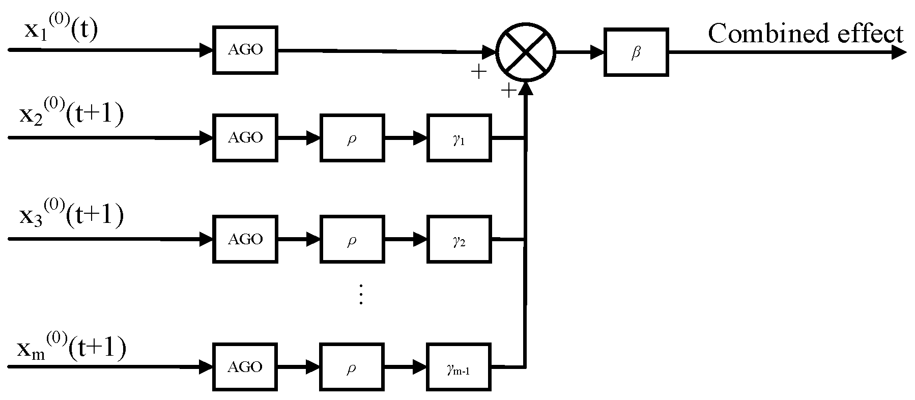
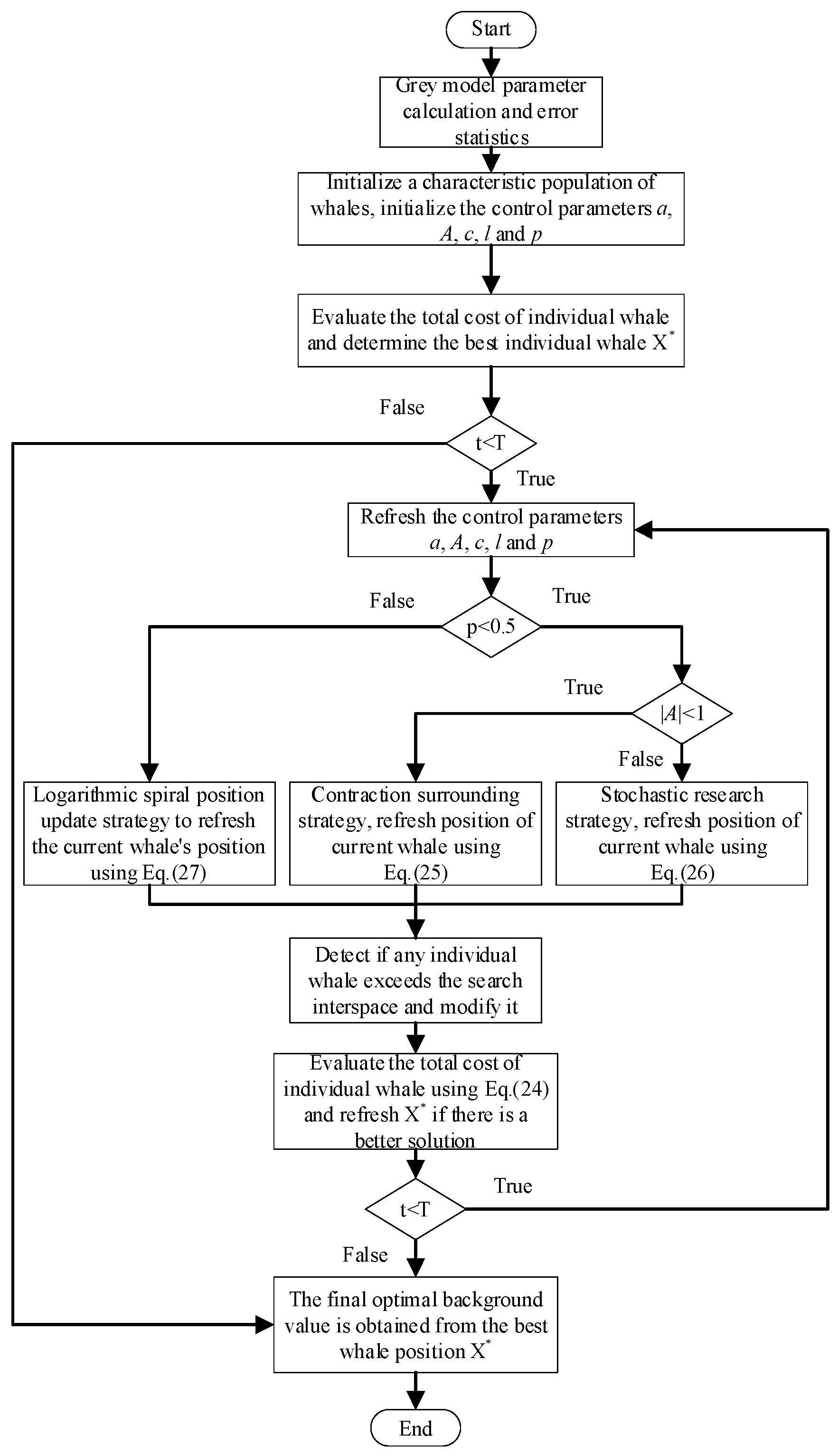
The evolution of deep displacement is characterized by stochasticity, nonlinearity, complexity, and uncertainty. In order to better predict the deep displacement propagation, it is necessary to fully consider the correlation between multiple sensing units of deep displacement. In this paper, based on grey system theory, a prediction method with feedback influence is proposed and the WOA is used to determine the unknown background value parameters in it.

(2)

By using three sensors’ data to show that the new grey prediction model has a smaller mean absolute percentage error, which is better than several comparative models. The input parameters in this process are the historical displacement-related parameters of the sensors above the slip band and the output is a prediction of the future displacement.

(3)

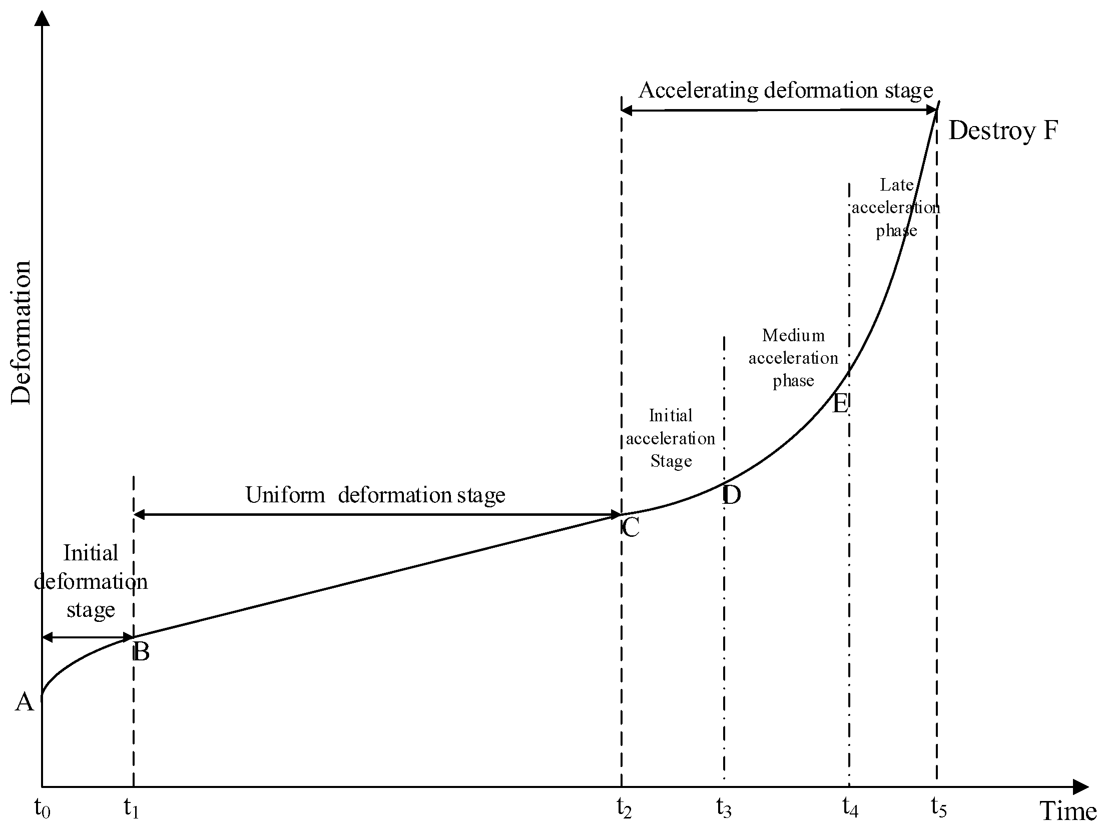
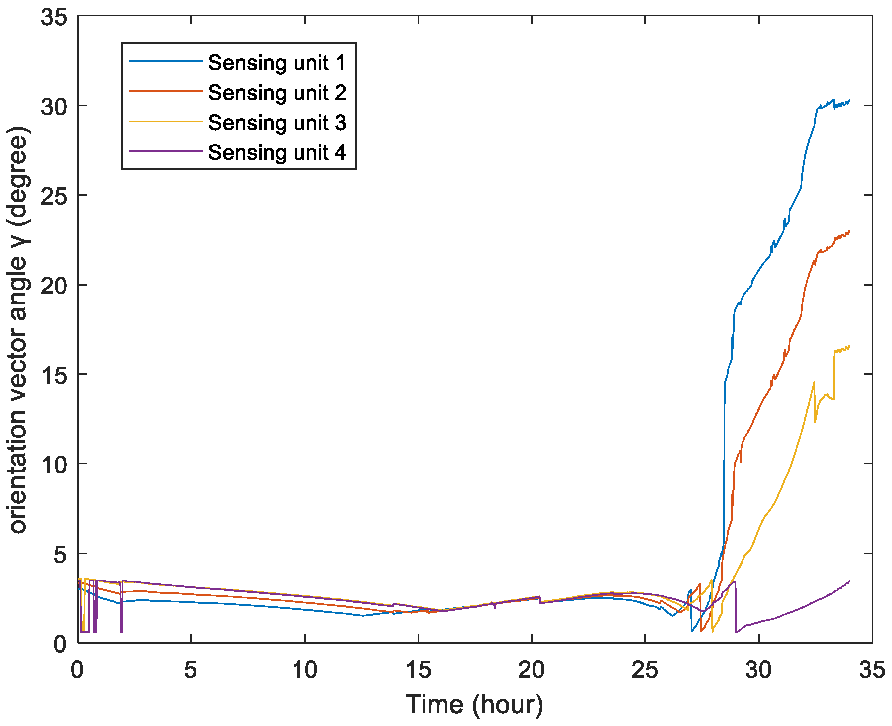
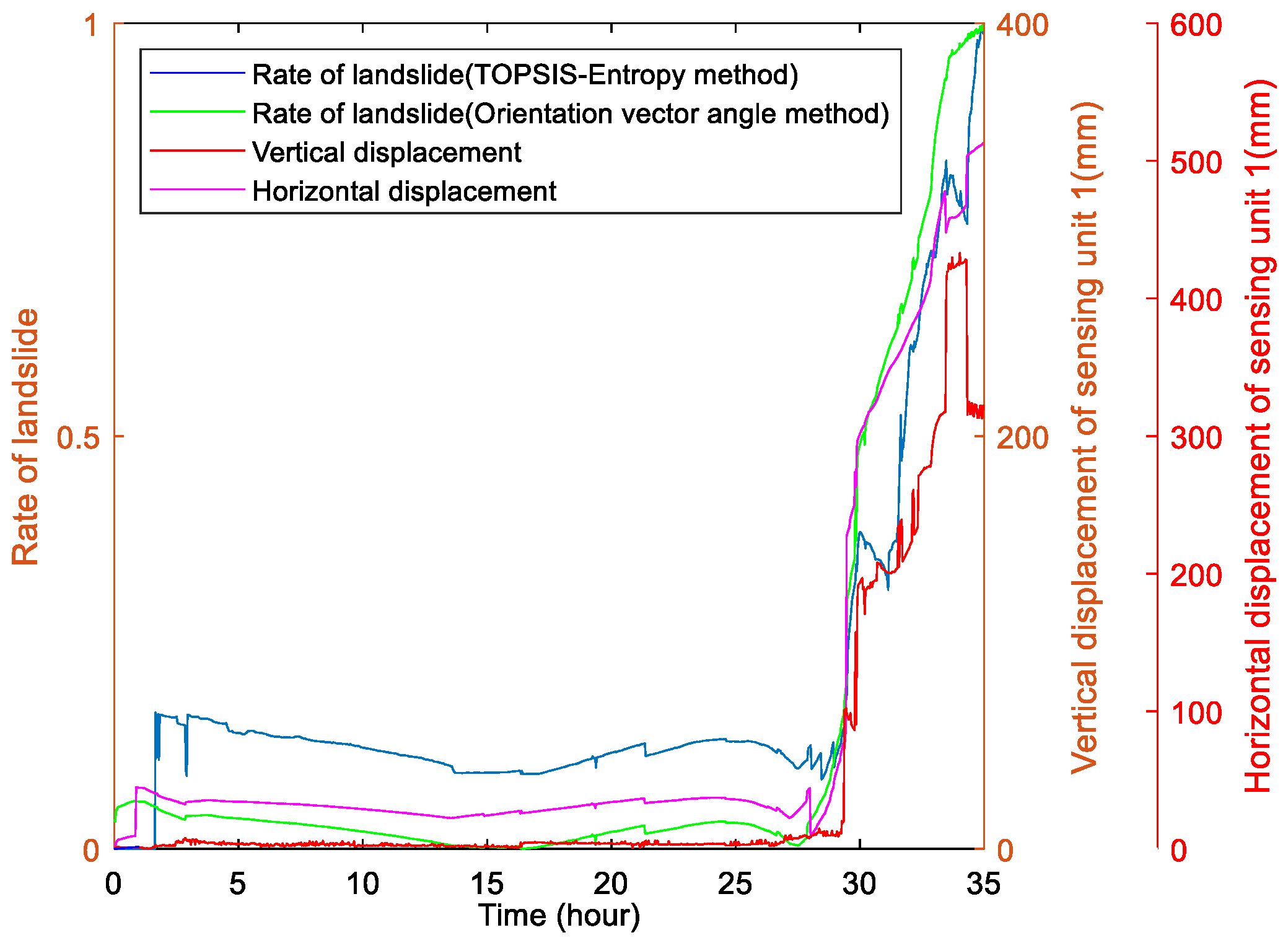
A new method for calculating landslide warning factors based on a deep displacement monitor sensor is proposed, which avoids the situation that it is difficult to have a unified standard due to complex environmental factors. Compared with the existing methods of evaluating landslide risk based on multi-parameter data, the orientation vector angle method can avoid the problem that landslide hazard factors are easily affected by data fluctuations. Therefore, it may be an effective method for general landslide displacement prediction.

Since the existing methods of weight selection are mainly contain the objective weighting and subjective weighting, how to assign an appropriate weight to different sensing units is an important issue. In addition, the displacement is only an obvious component in the landslide process, other factors, such as rainfall and hydrology, need to be considered together to improve the accuracy of the sensitivity analysis of the whole slope. Therefore, future work will not only focus on applying the proposed model to more landslide cases and practical applications, but also pay attention to optimizing the coefficient of orientation vector angle of different sensing units and taking other monitoring parameters into consideration.

References

1. Froude, M.J.; Petley, D.N. Global fatal landslide occurrence from 2004 to 2016. Nat. Hazards Earth Syst. Sci. 2018, 18, 2161–2181. [Google Scholar] [CrossRef] [Green Version]
2. Yan, T.; Shen, S.L.; Zhou, A.N.; Chen, J. A Brief Report of Pingdi Landslide (23 July 2019) in Guizhou Province, China. Geosciences 2019, 9, 368. [Google Scholar] [CrossRef] [Green Version]
3. Achu, A.L.; Joseph, S.; Aju, C.D.; Mathai, J. Preliminary analysis of a catastrophic landslide event on 6 August 2020 at Pettimudi, Kerala State, India. Landslides 2021, 18, 1459–1463. [Google Scholar] [CrossRef]
4. Ma, J.; Liu, X.; Niu, X.; Wang, Y.; Wen, T.; Zhang, J.; Zou, Z. Forecasting of Landslide Displacement Using a Probability-Scheme Combination Ensemble Prediction Technique. Int. J. Environ. Res. Public Health 2020, 17, 4788. [Google Scholar] [CrossRef]
5. He, C.; Hua, T.; Xiurun, G.; Yajun, L. Research on early warning of creep landslide by early-warning indictors based on deep displacements. Chin. J. Rock Mech. Eng. 2019, 38, 3015–3024. [Google Scholar] [CrossRef]
6. Zhu, X.; Xu, Q.; Zhou, J.; Deng, M. Remote Landslide Observation System with Differential GPS. Procedia Earth Planet. Sci. 2012, 5, 70–75. [Google Scholar] [CrossRef] [Green Version]
7. Benoit, L.; Briole, P.; Martin, O.; Thom, C.; Ulrich, P. Monitoring landslide displacements with the Geocube wireless network of low-cost GPS. Eng. Geol. 2015, 195, 111–121. [Google Scholar] [CrossRef]
8. Li, Y.; Zuo, X.; Xiong, P.; You, H.; Zhang, H.; Yang, F.; Zhao, Y.; Yang, Y.; Liu, Y. Deformation monitoring and analysis of Kunyang phosphate mine fusion with InSAR and GPS measurements. Adv. Space Res. 2022, 69, 2637–2658. [Google Scholar] [CrossRef]
9. Bányai, L.; Mentes, G.; Újvári, G.; Kovács, M.; Czap, Z.; Gribovszki, K.; Papp, G. Recurrent landsliding of a high bank at Dunaszekcső, Hungary: Geodetic deformation monitoring and finite element modeling. Geomorphology 2014, 210, 1–13. [Google Scholar] [CrossRef] [Green Version]
10. Rodgers, M.; Deng, F.; Dixon, T.H.; Glennie, C.L.; James, M.R.; Malservisi, R.; Van Alphen, R.; Xie, S. 2.03-Geodetic Applications to Geomorphology. In Treatise on Geomorphology, 2nd ed.; Shroder, J.F., Ed.; Academic Press: Oxford, UK, 2022; pp. 34–55. [Google Scholar] [CrossRef]
11. Gomberg, J.; Schulz, W.; Bodin, P.; Kean, J. Seismic and geodetic signatures of fault slip at the Slumgullion Landslide Natural Laboratory. J. Geophys. Res. 2011, 116. [Google Scholar] [CrossRef]
12. Marek, L.; Miřijovský, J.; Tuček, P. Monitoring of the Shallow Landslide Using UAV Photogrammetry and Geodetic Measurements; Springer: Cham, Switzerland, 2015. [Google Scholar]
13. Shimizu, Y.; Yamakoshi, T.; Osanai, N.; Fukushima, A.; Mio, A. Study on detection of landslide areas by differential interferometric synthetic aperture radar. J. Jpn. Landslide Soc. 2010, 42, 312–317. [Google Scholar] [CrossRef] [Green Version]
14. Song, C.; Yu, C.; Li, Z.; Pazzi, V.; Utili, S. Landslide geometry and activity in Villa de la Independencia (Bolivia) revealed by InSAR and seismic noise measurements. Landslides 2021, 18, 2721–2737. [Google Scholar] [CrossRef]
15. Zhu, Y.; Qiu, H.; Yang, D.; Liu, Z.; Sun, H. Pre- and post-failure spatiotemporal evolution of loess landslides: A case study of the Jiangou landslide in Ledu, China. Landslides 2021, 18, 3475–3484. [Google Scholar] [CrossRef]
16. Li, Z.; Cao, Y.; Wei, J.; Duan, M.; Wu, L.; Hou, J.; Zhu, J. Time-series InSAR ground deformation monitoring: Atmospheric delay modeling and estimating. Earth-Sci. Rev. 2019, 192, 258–284. [Google Scholar] [CrossRef]
17. Dai, K.R.; Liu, G.X.; Li, Z.H.; Ma, D.Y.; Wang, X.W.; Zhang, B.; Tang, J.; Li, G.Y. Monitoring Highway Stability in Permafrost Regions with X-band Temporary Scatterers Stacking InSAR. Sensors 2018, 18, 1876. [Google Scholar] [CrossRef] [Green Version]
18. Li, Y.; Huang, J.; Jiang, S.-H.; Huang, F.; Chang, Z. A web-based GPS system for displacement monitoring and failure mechanism analysis of reservoir landslide. Sci. Rep. 2017, 7, 17171. [Google Scholar] [CrossRef] [Green Version]
19. Peng, J.C.; Wang, S.L.; Zhang, Y.X.; Yue, T.; Song, Y. Application of borehole inclinometer in landslide deformation monitoring. J. Xi’an Univ. Sci. Technol. 2014, 34, 440–444. [Google Scholar]
20. Kaya, A.; Mdll, Ü.M. Slope stability evaluation and monitoring of a landslide: A case study from NE Turkey. J. Mt. Sci. 2020, 17, 2624–2635. [Google Scholar] [CrossRef]
21. Ccc, A.; Cpl, B.; Yin, J.; Wcl, B.; Csy, B. Improved technical guide from physical model tests for TDR landslide monitoring. Eng. Geol. 2022, 296, 106417. [Google Scholar]
22. Ho, S.C.; Chen, I.H.; Lin, Y.S.; Chen, J.Y.; Su, M.B. Slope deformation monitoring in the Jiufenershan landslide using time domain reflectometry technology. Landslides 2019, 16, 1141–1151. [Google Scholar] [CrossRef]
23. Lin, Y.S.; Chen, I.H.; Ho, S.C.; Chen, J.Y.; Su, M.B. Applying time domain reflectometry to quantification of slope deformation by shear failure in a landslide. Environ. Earth Sci. 2019, 78, 1–11. [Google Scholar] [CrossRef]
24. Zhang, L.; Shi, B.; Zhang, D.; Sun, Y.; Inyang, H.I. Kinematics, triggers and mechanism of Majiagou landslide based on FBG real-time monitoring. Environ. Earth Sci. 2020, 79, 1–17. [Google Scholar] [CrossRef]
25. Pei, H.; Peng, C.; Yin, J.; Zhu, H.; Chen, X.; Pei, L.; Xu, D. Monitoring and warning of landslides and debris flows using an optical fiber sensor technology. J. Mt. Sci. 2011, 8, 11. [Google Scholar] [CrossRef]
26. Wu, Z.S.; Xu, B.; Takahashi, T.; Harada, T. Performance of a BOTDR optical fibre sensing technique for crack detection in concrete structures. Struct. Infrastruct. Eng. 2008, 4, 311–323. [Google Scholar] [CrossRef]
27. Ran, Q.H.; Su, D.Y.; Qian, Q.; Fu, X.D.; Wang, G.Q.; He, Z.G. Physically-based approach to analyze rainfall-triggered landslide using hydraulic gradient as slide direction. J. Zhejiang Univ. A 2012, 13, 943–957. [Google Scholar] [CrossRef]
28. Yavari-Ramshe, S.; Ataie-Ashtiani, B. A rigorous finite volume model to simulate subaerial and submarine landslide-generated waves. Landslides 2015, 14, 1–19. [Google Scholar] [CrossRef]
29. Chen, G.; Meng, X.M.; Guo, P.; Ya-Jun, L.I.; Zeng, R.Q. Landslide susceptibility mapping based on GIS and information value model in Bailong river basin. J. Lanzhou Univ. (Nat. Sci.) 2011, 47, 1–6. [Google Scholar]
30. Chen, W.; Li, W.; Hou, E.; Zhao, Z.; Deng, N.; Bai, H.; Wang, D. Landslide susceptibility mapping based on GIS and information value model for the Chencang District of Baoji, China. Arab. J. Geosci. 2014, 7, 4499–4511. [Google Scholar] [CrossRef]
31. Sharma, L.P.; Patel, N.; Ghose, M.K.; Debnath, P. Development and application of Shannon’s entropy integrated information value model for landslide susceptibility assessment and zonation in Sikkim Himalayas in India. Nat. Hazards 2015, 75, 1555–1576. [Google Scholar] [CrossRef]
32. Singh, P.; Sharma, A.; Sur, U.; Rai, P.K. Comparative landslide susceptibility assessment using statistical information value and index of entropy model in Bhanupali-Beri region, Himachal Pradesh, India. Environ. Dev. Sustain. A Multidiscip. Approach Theory Pract. Sustain. Dev. 2021, 23, 5233–5250. [Google Scholar] [CrossRef]
33. Li, X.; Tang, H.; Chen, S. Application of GIS-Based Logistic Regression Model and Cluster Method to Regional Landslide Risk Zoning. In Geological Engineering: Proceedings of the 1st International Conference (ICGE 2007); ASME Press: New York, NY, USA, 2009. [Google Scholar]
34. Sun, D.; Wen, H.; Zhang, Y.; Xue, M.; Glade, T.; Murty, T.S. An optimal sample selection-based logistic regression model of slope physical resistance against rainfall-induced landslide. Nat. Hazards 2021, 105, 1255–1279. [Google Scholar] [CrossRef]
35. Xiao, Y.; Xian-Fu, L.I. Forecast for landslide based on Optimum Grey model. J. Wuhan Inst. Technol. 2012, 34, 31–35. [Google Scholar]
36. Miao, S.; Hao, X.; Guo, X.; Wang, Z.; Liang, M. Displacement and landslide forecast based on an improved version of Saito’s method together with the Verhulst-Grey model. Arab. J. Geosci. 2017, 10, 53. [Google Scholar] [CrossRef]
37. Mowen, X. Prediction of Landslide Deformation dy Dynamic Unequal Interval Grey Model. Met. Mine 2013, 42, 20. [Google Scholar]
38. Li, S.H.; Zhu, L.; Wu, Y.; Lei, X.Q. A novel grey multivariate model for forecasting landslide displacement. Eng. Appl. Artif. Intell. 2021, 103, 104297. [Google Scholar] [CrossRef]
39. Youssef, A.M.; Pourghasemi, H.R.; Pourtaghi, Z.S.; Al-Katheeri, M.M. Landslide susceptibility mapping using random forest, boosted regression tree, classification and regression tree, and general linear models and comparison of their performance at Wadi Tayyah Basin, Asir Region, Saudi Arabia. Landslides 2016, 13, 839–856. [Google Scholar] [CrossRef]
40. Chen, W.; Li, X.; Wang, Y.; Chen, G.; Liu, S. Forested landslide detection using LiDAR data and the random forest algorithm: A case study of the Three Gorges, China. Remote Sens. Environ. 2014, 152, 291–301. [Google Scholar] [CrossRef]
41. Zhou, X.; Wen, H.; Zhang, Y.; Xu, J.; Zhang, W. Landslide susceptibility mapping using hybrid random forest with GeoDetector and RFE for factor optimization. Geosci. Front. 2021, 12, 101211. [Google Scholar] [CrossRef]
42. Xu, Z.W. GIS and ANN model for landslide susceptibility mapping. J. Geogr. Sci. 2001, 11, 374–381. [Google Scholar]
43. Yilmaz, I. Landslide susceptibility mapping using frequency ratio, logistic regression, artificial neural networks and their comparison: A case study from Kat landslides (Tokat—Turkey). Comput. Geosci. 2009, 35, 1125–1138. [Google Scholar] [CrossRef]
44. Mehrabi, M.; Moayedi, H. Landslide susceptibility mapping using artificial neural network tuned by metaheuristic algorithms. Environ. Earth Sci. 2021, 80, 1–20. [Google Scholar] [CrossRef]
45. Shentu, N.; Wang, F.; Li, Q.; Qiu, G.; Tong, R.; An, S. Three-Dimensional Measuring Device and Method of Underground Displacement Based on Double Mutual Inductance Voltage Contour Method. Sensors 2022, 22, 1725. [Google Scholar] [CrossRef]
46. Tien, T.L. A research on the grey prediction model GM(1,n). Appl. Math. Comput. 2012, 218, 4903–4916. [Google Scholar] [CrossRef]
47. Zeng, B.; Luo, C.; Liu, S.; Bai, Y.; Li, C. Development of an optimization method for the GM(1,N) model. Eng. Appl. Artif. Intell. 2016, 55, 353–362. [Google Scholar] [CrossRef]
48. Tan, G.J. The Structure Method and Application of Background Value in Grey System GM(1,1) Model (II). Syst. Eng. Theory Pract. 2000, 20, 98–103. [Google Scholar]
49. Yang, Y.; Liu, S. Grey Systems: Theory and Application. Grey Syst. Theory Appl. 2011, 4883, 44–45. [Google Scholar]
50. Mirjalili, S.; Lewis, A. The Whale Optimization Algorithm. Adv. Eng. Softw. 2016, 95, 51–67. [Google Scholar] [CrossRef]
51. Xu, Q.; Tang, M.; Xu, K.; Huang, X. Research on space-time evolution laws and early warning-prediction of landslides. Yanshilixue Yu Gongcheng Xuebao/Chin. J. Rock Mech. Eng. 2008, 27, 1104–1112. [Google Scholar]
52. Shu, H.E.; Chen, F. Research of landslide stability assessment based on intuitionistic fuzzy sets TOPSIS multiple attribute decision making method. Chin. J. Geol. Hazard Control 2016, 27, 22–28. [Google Scholar]
53. Seif, A.; Mofrad, M.R. Examining the potential landslide in Chaharmahal Va Bakhtiari province by applying multi criterion models of decision making. Trans. R. Soc. Edinb. Earth Sci. 2013, 26, 31–48. [Google Scholar]
Figure 1. Schematic diagram of the framework of the landslide experiment equipment.
Applsci 13 00213 g001
Figure 2. Details of the geotechnical disaster simulator box (a) Top view of the earth loading box (b) Front view of the box (c) Right view of the earth loading box (d) Back view of the earth loading box Rainfall-induced landslides are the most common type of landslide. Rainfall destabilizes slopes by changing the physical properties of the slope as well as the groundwater level to reduce the shear strength of the soil. The whole device is designed to simulate continuous rainfall on the slope from several hours to tens of hours.
Applsci 13 00213 g002
Figure 3. Details of rainfall and groundwater equipment (a) Rainfall equipment (b) Groundwater simulation equipment.
Applsci 13 00213 g003
Figure 4. Details of the deep displacement monitor sensor.
Applsci 13 00213 g004
Figure 5. Schematic diagram of double mutual inductance voltage method.
Applsci 13 00213 g005
Figure 6. Details of multi-factor information collection.
Applsci 13 00213 g006
Figure 7. Flow chart of background value optimization.
Applsci 13 00213 g007
Figure 8. Sketch of three stages of slope deformation.
Applsci 13 00213 g008
Figure 9. Sketch of the angle between the horizontal cumulative displacement and the vertical cumulative displacement.
Applsci 13 00213 g009
Figure 10. Initial state diagram of experiment. (a) Description of the initial state of the entire deep displacement monitor sensor on the slope. (b) Show a 1 m high slope with a 20 cm high plane to simulate the toe of the slope (c) A sectional view of the distribution of the integrated deep displacement three-dimensional measuring sensor buried in the slope.
Applsci 13 00213 g010
Figure 11. Curve of actual depth deformation.
Applsci 13 00213 g011
Figure 12. Curve of accumulative deformation. (a) Graph of cumulative horizontal displacement versus time (b) Graph of cumulative vertical displacement versus time.
Applsci 13 00213 g012
Figure 13. The curve of original displacement data. (a) Graph of original horizontal displacement versus time. (b) Graph of original vertical displacement versus time.
Applsci 13 00213 g013
Figure 14. The curve of prediction for sensing unit 1. (a) Graph of horizontal displacement prediction effect of sensing unit 1. (b) Graph of vertical displacement prediction effect of sensing unit 1.
Applsci 13 00213 g014
Figure 15. Curve of prediction for sensing unit 2. (a) Graph of horizontal displacement prediction effect of sensing unit 2. (b) Graph of vertical displacement prediction effect of sensing unit 2.
Applsci 13 00213 g015
Figure 16. Curve of prediction for sensing unit 4. (a) Graph of horizontal displacement prediction effect of sensing unit 4. (b) Graph of vertical displacement prediction effect of sensing unit 4.
Applsci 13 00213 g016
Figure 17. The curve of orientation vector angle.
Applsci 13 00213 g017
Figure 18. The curve of danger rate of landslide.
Applsci 13 00213 g018