Article

A New Competitive Neural Architecture for Object Classification

1
Mathematics Informatics & Communications Systems Laboratory, Cadi Ayyad University, Marrakech 40000, Morocco
2
Center for Sensing Applications (CRSA), Mohammed VI Polytechnic University (UM6P), Ben Guerir 43150, Morocco
3
Information Processing Laboratory, Ben M’Sik Faculty of Sciences, Hassan II University of Casablanca (UH2C), Casablanca 20670, Morocco
*
Author to whom correspondence should be addressed.
Appl. Sci. 2022, 12(9), 4724; https://doi.org/10.3390/app12094724
Submission received: 25 January 2022 / Revised: 21 April 2022 / Accepted: 25 April 2022 / Published: 7 May 2022
(This article belongs to the Section Computing and Artificial Intelligence)

Abstract

:
In this paper, we propose a new neural architecture for object classification, made up from a set of competitive layers whose number and size are dynamically learned from training data using a two-step process that combines unsupervised and supervised learning modes. The first step consists in finding a set of one or more optimal prototypes for each of the c classes that form the training data. For this, it uses the unsupervised learning and prototype generator algorithm called fuzzy learning vector quantization (FLVQ). The second step aims to assess the quality of the learned prototypes in terms of classification results. For this, the c classes are reconstructed by assigning each object to the class represented by its nearest prototype, and the obtained results are compared to the original classes. If one or more constructed classes differ from the original ones, the corresponding prototypes are not validated and the whole process is repeated for all misclassified objects, using additional competitive layers, until no difference persists between the constructed and the original classes or a maximum number of layers is reached. Experimental results show the effectiveness of the proposed method on a variety of well-known benchmark data sets.

1. Introduction

Machine learning is a form of artificial intelligence that makes it possible to design systems capable of learning from examples, without explicit programming or direct human intervention. It is an efficient tool for analyzing highly complex data, such as those encountered in object recognition and control problems [1,2,3], in order to extract relevant information or reveal hidden patterns [4,5]. Machine learning also allows the conversion of hard optimization problems into satisfaction problems, where the aim becomes the search for acceptable or satisfactory solutions in reasonable amounts of time. In this work, we are interested in the machine learning problem of object classification using competitive neural networks [6]. For this, we propose a new competitive neural network architecture and a new process for training it to perform object classification tasks.
Training a neural network consists in adjusting its synaptic weights, including biases, to correctly accomplish a classification, clustering or regression task. In the particular case of classification tasks, the goal of the training process is to find the set of synaptic weights that minimizes the classification error rate, which globally measures the difference between real and network-generated labels of all training examples. In other words, these synaptic weights can be viewed as parameters that define the separating boundaries between classes in the data space [7,8]. Mathematically speaking, the training process of a neural network on a classification task, using a training data set X, is an optimization process aimed at minimizing the cost function defined by [9]:
J ( X , S ) = x k X d ( y k , S ( x k ) )
where y k is the true label of the input x k ; S ( x k ) is the output of the last layer of the neural network related to x k ; and d is the difference between y k and S ( x k ) .
For clustering problems, the aim is rather to find a set of prototypes that can be used as representatives for the c clusters that form the training data set. These prototypes can then be used for the purpose of labeling new and unseen objects using a decision rule, such as the nearest prototype rule (1NP) [10,11,12]. To assess the quality of clustering results, we generally use objective functions that measure the similarity and separability of clusters [13,14,15]. More specifically, a clustering algorithm can be defined as an optimization process for minimizing the following cost function:
J ( X , W ) = x k X i = 1 c u ( k , i ) d ( x k , w i )
where W is the weight matrix of the neural network; u ( k , i ) is the membership degree of object k to cluster i; and w i is the weight vector of the neuron that represents the prototype of cluster i, with 1 i c .
One major problem in training neural networks is the initialization of hyper parameters, such as the number of layers and neurons per layer, the learning rate, and the number and size of convolution and pooling filters in the case of convolutional neural networks [6,9,16]. The goal of this work is to propose a new neural architecture composed of a set of competitive layers whose number and size can be automatically learned from data, and for which satisfactory initial values of algorithmic parameters can be easily found.
Each layer in the proposed architecture is a competitive layer composed of a set of nodes that represent class prototypes and that are trained in unsupervised mode. The synaptic weights of each node represent the components of a class prototype in the data space. Once determined, these prototypes are used as a basis for the nearest prototype rule in the process of reconstructing the c classes of the training data set. The resulting classes are then compared to the original classes and all misclassified objects, if any, are submitted to an additional competitive layer that will try to correctly classify them, and so on, until all objects are well-classified or a maximum number of competitive layers is reached. This is why we call the proposed architecture a multi-competitive-layer neural network (MCLNN). In the next section, we provide more detailed information about the components of this architecture, starting with a reminder on the concepts of formal neurons, competitive neural networks, as well as traditional unsupervised algorithms commonly used for training this particular type of neural network. We then explain how the proposed architecture is built up from these components, and how it is trained on the task of object classification using the examples of a training data set.

2. Proposed Method

2.1. Formal Neurons as Cluster Prototypes

Cluster prototypes are represented by formal neurons that form the different competitive layers of the proposed neural architecture. During the training process, for each input vector x, the activation function used by each neuron or prototype v in the current layer is the distance measure between x and v defined by the expression:
φ ( x ) = | | v x | | 2 = j = 1 p v j x j 2
where x j and v j denote the jth component of x and v, respectively, and p is the dimension of the data space, i.e., the number of features per object vector.

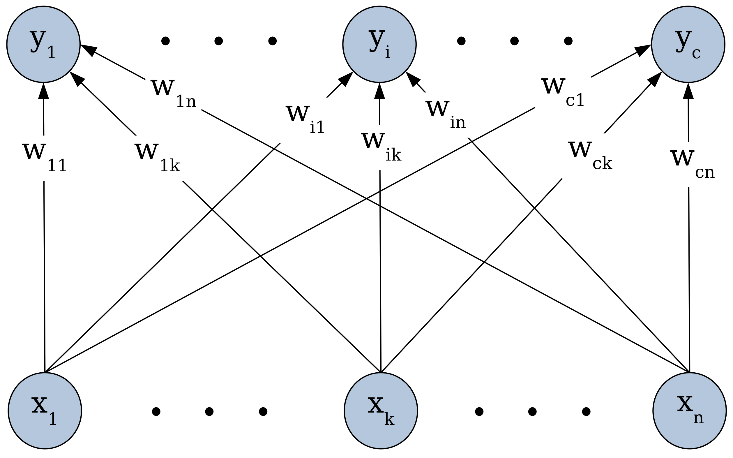
2.2. Competitive Neural Networks

A competitive neural network (Figure 1) is comprised of only two layers: an input layer of p neurons aimed at receiving the input data in the form of p-dimensional object vectors, and an output or competitive layer composed of c neurons representing each cluster prototype.
Traditional algorithms for training competitive neural networks, whose state of the art can be represented by the unsupervised learning vector quantization algorithm (LVQ3) [17], are based on the principle of the winner takes all (WTA) [17,18]. Meaning that, for each input vector x presented to the network during its training process, only one output neuron, called the winner, is adjusted by assigning x to the cluster it represents. It is the neuron whose weight vector minimizes the distance to x. The performance of such algorithms is limited to situations where the c clusters are compact and well separated.
For overlapping or not well separated clusters, many generalizations of WTA algorithms are proposed in the literature, including different variants of the fuzzy learning vector quantization algorithm (FLVQ) [19,20,21], which can be considered as the state of the art of these generalizations. FLVQ, whose operating principle is recalled in the next subsection, is mainly inspired by the well-known fuzzy c-means algorithm, FCM [22].

2.3. The Fuzzy Learning Vector Quantization (FLVQ)

FLVQ is a fuzzy variant of LVQ3 for which all neurons are winners but to different degrees. It is an optimization procedure that tries to better exploit the structural information carried by each training example [20] by minimizing the following objective function
J m ( U , V , X ) = k = 1 n i = 1 c ( u i k ) m x k v i 2
where U is a matrix of membership degrees, with u i k denoting the membership degree of the kth object to the ith class; V is the matrix of prototypes, with v i representing the ith class prototype; m > 1 is a weighting exponent that controls the fuzziness degree of candidate partitions during the learning process; and n is the total number of training examples.
J m can be interpreted as a fuzzy measure of the global error incurred in representing the n training vectors by the c prototypes. It can be minimized using an alternating optimization procedure that consists in repeatedly recalculating U and V matrices using the expressions:
u i k , t = l = 1 c x k v i , t 2 x k v l , t 2 1 m 1 1
and
v i , t = k = 1 n ( u i k , t ) m x k k = 1 n ( u i k , t ) m
Hence, starting from a randomly chosen matrix of initial prototypes V 0 = v 1 , 0 , v 2 , 0 , , v c , 0 , if we iteratively recalculate the components of U and V according to (5) and (6), the process will converge to a point ( U * , V * ) where the c prototypes are stabilized, which means a point from which the difference V t V t 1 becomes insignificant. To evaluate this difference, we use the expression:
V t V t 1 = max 1 i c max 1 j p | v i j , t v i j , t 1 |
Depending on the way m varies throughout iterations, two versions of FLVQ have been developed: FLVQ↓ and FLVQ↑. In FLVQ↓, m decreases according to the relation
m = m t = m m a x t t m a x m m a x m m i n
and in FLVQ↑, it increases according to
m = m t = m m i n + t t m a x m m a x m m i n
where t is the index of iterations and t m a x the maximal number of iterations.

2.4. Training Process of the Proposed Architecture

The first step in the training algorithm of the proposed neural architecture is an unsupervised learning procedure that uses the FLVQ algorithm for representing each class by one or more prototypes that the procedure tries to learn from the training data in unsupervised mode, i.e., without using the known labels. The second step uses a supervised learning procedure for assessing the quality of the learned prototypes in terms of classification results. For this, the c classes are reconstructed using the nearest prototype rule, and the obtained results compared to the original classes. If one or more constructed classes differ from the original ones, the corresponding prototypes are rejected and both steps are repeated for these classes using additional competitive layers until no difference persists between the constructed and the original classes, or a maximal number of layers is reached. For this, all misclassified objects are grouped with those, if any, that present small membership degrees to all classes in order to form the training data set for an additional layer of competitive neurons.
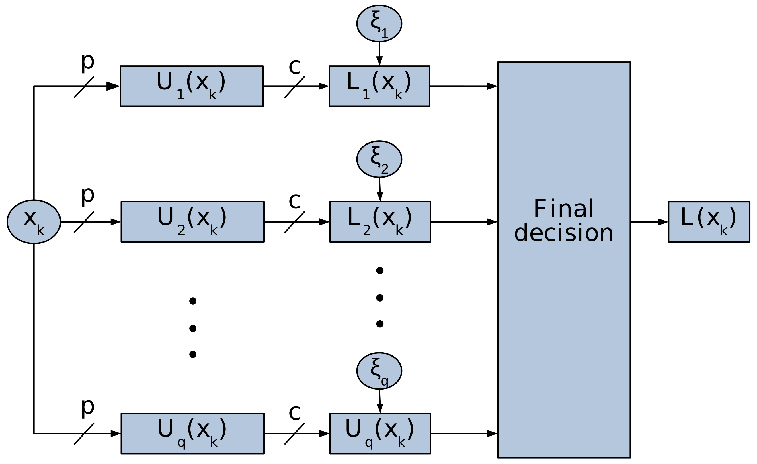
As shown in (Figure 2), the resulting architecture is a multi-competitive-layer neural network (MCLNN). Each of these layers contains c r neurons representing the c r detected prototypes, and s r possible additional neurons representing the training examples that could not be correctly classified by this layer. These remaining examples are called “strong elements” and can be seen as noisy elements for the current layer.
Thus, the ultimate goal of MCLNN is to represent each class by a set of one or more prototypes. The total number of the resulting prototypes for all layers of the network is c t o t = r = 1 q c r , with c c t o t . During the learning process of these prototypes, whenever an object is presented to the input of a layer r, all neurons of this layer are considered as winners to different degrees, and the membership degrees of the input object to the corresponding classes are computed using the expression:
u r i ( x r k ) = l = 1 c r φ r i ( x r k ) φ r l ( x r k ) 2 m 1 1
where u r i ( x r k ) is the membership degree of the object x r k to the cluster C r i , which is represented by the ith neuron of the rth layer; c r is the number of neurons in the rth layer; x r k is the kth object vector of the training data set used to train the rth layer; x r k j is the jth feature of the object vector x r k ; m > 1 is a weighting exponent that controls the fuzziness degree of candidate partitions during the learning process; and φ r i ( x r k ) is the activation function of the i t h neuron of the rth layer, defined by the expression:
φ r i ( x r k ) = | | v r i x r k | | 2 = j = 1 p v r i j x r k j 2
where v r i j is the jth synaptic weight of neuron r i , which is also the jth feature of prototype v r i that represents cluster C r i ; p is the number of features of the object vectors; i is the index used to locate a neuron in a competitive layer; and r is the layer’s index.
The first layer is trained using the original training data set X, and each subsequent one with the set of remaining strong elements X r . Thus, at the end of the training process of each layer r, all objects of its training data set X r are labeled. For this, each object x r k in X r is assigned to the cluster C r i represented by the winning prototype, which is the output neuron that maximizes u r i ( x r k ) while exceeding a certain threshold ζ r . The latter is introduced in this work to ensure a minimum of similarity between each processed object, and the representative prototype of the class it is assigned to, using the maximum membership degree rule. Consequently, two possible cases can be distinguished according to the label Γ ( r , i ) of x r k : (1) x r k is well classified, if its true label L ( x r k ) is equal to Γ ( r , i ) , or (2) x r k is misclassified, if L ( x r k ) Γ ( r , i ) .
In the first case, the rth layer is used to recognize x r k , and we say that x r k accepts its representation by the winning neuron of the rth layer. In the second case, the classification result is ignored because x r k cannot be represented by the winning neuron. In this case, x r k is considered as a strong element that leads to the addition of a new neuron to MCLNN that may better represent it. For this, the p synaptic weights of the newly added neuron are initialized using the p components of x r k .
In the instance where the membership degree of x r k to the class represented by the winning prototype in the current layer does not reach its acceptance threshold ζ r , we consider that x r k cannot be classified at the level of this layer and we assign it to a new training data set that will be used for training the next additional layer, r + 1 .
This mechanism can be summarized by the following mathematical expression:
L r ( x r k ) = { (12a) 1   i f   max l ( u r l ( x r k ) ) < ζ r (12b) Γ ( r , argmax l ( u r l ( x r k ) ) )   otherwise
where L r ( x r k ) is the label of the object x r k generated by the r t h layer. If L r ( x r k ) = 1 , x r k and all similar objects cannot be processed by this layer; a r g m a x l u r l ( x r k ) is the maximum membership degree of x r k to all clusters; Γ r , i is the label of cluster C r i represented by neuron i of layer r; and ζ r is the minimum threshold of membership degree for x r k to accept to be represented exclusively by a neuron of the current layer. Any result of classification generated by other layers is then ignored.
The number of layers used to form the MCLNN depends on the learning outcomes of the first layers. Indeed, if the first layers allow the correct classification of all training examples, there will be no need for additional layers and the training process of MCLNN is terminated. In the presence of misclassified objects, however, the validation step will group all these objects with those, if any, that present small membership degrees to all classes, in order to form the training data set for the next additional layer. This process is iterated until all objects are well classified or a maximum number of layers is reached. Our simulation results show that, for all the studied data examples, all objects could be well classified before reaching the fixed maximum of 20 layers (Table 1).
A more formal description of this hybrid learning algorithm is given by the following pseudo-code:
Given a set of n training examples X = { x 1 , , x n } R p ;
  • Step 1: Construct a neural network of one competitive layer with c neurons (So far, r = 1 , c r = c and X r = X );
  • Step 2: Initialize ζ 0 by a value in [ 0 , 1 ] ;
  • Step 3: Initialize the step δ with a value in [ 0 , ζ 0 ] ;
  • Step 4: Apply FLVQ to train the layer r using the data set X r ; This step ends with the convergence of FLVQ;
  • Step 5: Adjust ζ r by ζ r 1 + ( r 1 ) δ ;
  • Step 6: For each object x r k of the data set X r presented to the input of the current layer r:
  • Evaluate the activation function of each neuron i ( i = 1 , , c r ) of the layer r using the Equation (11);
  • Evaluate the membership degrees of the object x r k to all clusters represented by the neurons of the layer r, using the Equation (10);
  • Find the maximum membership degree u r i ( x r k ) for i = 1 , , c r ;
  • If m a x i u r i ( x r k ) ζ r :
    -
    Evaluate the label L r ( x r k ) using the Equation (Section 2.4);
    -
    if L r ( x r k ) L ( x r k ) :
    Add a new neuron to the layer r;
    Increase the size of the layer r ( c r = c r + 1 );
    Write the features of x r k in the weights of the new neuron ( v c r + 1 = x r k );
  • else
    -
    Create the set of examples X r + 1 = ϕ R p if it does not exist;
    -
    Add the object x r k to the dataset X r + 1 ;
  • Step 7: If X r + 1 ϕ :
  • Increment r ( r = r + 1 );
  • Allocate c r neurons to form a new layer r;
  • Use the data set X r as training data set for the layer r;
  • Go to step 4;
  • Step 8: Return the final result, which is the global architecture and the synaptic weights of all of its neurons.
Using the big O notation, the computational complexity of each layer L of the proposed architecture at each iteration is given by the expression O( c L .p. n L ), where c L denotes the number of classes in the training data set of layer L, which is also the number of neurons in layer L, and n L is the number of elements of this data set. For the N layers of the whole network, and the total number of iterations required for convergence, t, this amounts, in the worst case, to O(t. c 2 .p.n.N). Remarking that c L < c and N < < n , we can conclude that this is the same order as O(t. c 2 .p.n), which is the computational complexity of the state of the art method, FLVQ.
During the exploitation phase, the label assigned to each input object x r k is generated by the first layer whose result is taken into account by an object x; i.e.,:
L ( x ) = L r ( x ) , r = min l = 1 , . . , q ( l ) such   as L r 1
where q is the number of competitive layers forming MCLNN; L ( x ) is the final label of the object x generated by the proposed neural architecture.
The following pseudo-code provides a more formal description of the exploitation process:
For each object x presented to MCLNN for recognition;
  • Step 1: Initialize the used layer’s index by r = 1 ;
  • Step 2: Present the object vector x to the input of the layer r;
  • Step 3: Evaluate the activation function of each neuron i ( i = 1 , , c r ) of the current layer using the Equation (11);
  • Step 4: Evaluate the membership degrees of x to all clusters represented by the neurons of the current layer using the Equation (10);
  • Step 5: Evaluate the label L r ( x ) using the Equation (Section 2.4);
  • Step 6:
  • If L r ( x ) 1 :
    -
    the final label is L ( x ) = L r ( x ) ;
  • else:
    -
    Increment r ( r = r + 1 );
    -
    Evaluate
    u r , m a x = m a x ( u r 1 , m a x , m a x ( u r l ( x ) l = 1 , . . , c r ) ) ;
    -
    If layer r is the last layer:
    L ( x ) = a r g ( u r , m a x ) ;
    -
    else:
    go to step 3;
  • Step 7: Return L ( x ) .

3. Results and Discussion

3.1. The Used Data Sets

In order to test the robustness of the proposed neural architecture, in this section, we present the results of its application to a selection of 13 benchmark data sets widely used in the literature, and we compare these results to those produced by other methods. The selected data sets differ in nature and size and are related to different application domains. Each data set was split into two subsets used, respectively, for the training process and the test of generalization on unseen examples. More information about these data, including their source and the number of elements in each subset, are provided in Table 2.

3.2. Examples of Generated Prototypes and Extracted Strong Elements

In order to explain the classification process using MCLNN in a practical way, we use in this section the Iris data set, and we show by numerical data and graphical diagrams the positions of the learned prototypes and the extracted strong elements.
The Iris dataset contains 150 examples of Iris flowers originated from three different classes, each represented by a vector of four measurements. To visually present this dataset, we choose to use 2D projections (Figure 3).
Regardless of the used projection and the selected features, it is easy to see that one of the three Iris classes is well separated from the other two, which are very overlapping. We note that the main difficulty in classifying the Iris data consists in separating the two overlapping classes.
Among 192,000 simulations carried out by classification of the Iris data, according to the proposed learning scheme, we select two different simulations giving an error rate equal to 0 (Table 3), and we illustrate the learned prototypes and the extracted strong elements. The meaning of the parameters given in Table 3 are: m is the initial value of the fuzziness factor; ζ is the acceptance threshold for the processed object to be classified by the first competitive layer; δ is the acceptance step used to adjust the acceptance threshold through iterations; C t o t is the total number of neurons in MCLNN; C r is the number of neurons of the rth layer; S t o t is the total number of strong elements extracted after training MCLNN; and S r is the number of strong elements extracted by the rth layer.
The first simulation gives five prototypes and 15 strong elements (Table 4), and simulation 2, two more prototypes and only three strong elements (Table 5). The positions of these prototypes and strong elements are graphically represented in Figure 4.
We note that the well separated class is represented by a single prototype in the two simulations, while the two overlapping classes are represented by more than one prototype. Moreover, all strong elements belong exclusively to the two overlapping classes. In fact, strong elements can be seen as objects that cannot be correctly classified based on the prototypes directly learned by the layers of MCLNN. These elements are considered as noisy objects and do not contribute to the adjustment of the prototypes.

3.3. Performance Evaluation and Comparison with Other Methods

To evaluate the performance of the proposed architecture in predicting the labels of new objects based on the learned prototypes, and compare this performance with other methods, two performance measures are used: (1) the error rate, or percentage of misclassified objects, which is computed for both training and test datasets, and (2) the sensitivity to parameter initialization, measured for each parameter by the largest interval of initial values that lead to the best results.
For the sake of comparisons, these two performance measures are evaluated on different benchmark datasets for three well-known other algorithms, namely the learning vector quantization algorithm, LVQ1, the multilayer perceptron, MLP, and the support vector machine algorithm, SVM. Like the proposed method, the first algorithm, LVQ1, is also a prototype generator, while MLP tries to find non-linear separations between the c classes in the data space, and SVM the best possible separation boundaries among the c classes.
To evaluate the error rate, we use the expression:
E r r = k = 1 n E k n × 100 %
where E k is equal to 1 if the object k is misclassified, and to 0 otherwise; n is the number of objects of the used dataset.
The best error rate is the smallest value obtained over 192,000 simulations for each method and each dataset. The algorithmic parameters used during these simulations for each algorithm are shown in Table 6.
As shown by Table 7, the only algorithm for which the error rate is null for all training datasets is MCLNN. The second best performance in terms of error rate for the training datasets is obtained by the SVM algorithm, for which the error rate is different from zero for only three cases. This is not surprising given the way the prototypes and the separating boundaries are determined in MCLNN and SVM, respectively.
Similar results are obtained on the test datasets, for which both MCLNN and SVM outperform the remaining two algorithms in the ability to generalize the learned classification task to correctly predict the labels of new objects, that were not seen during the training process (Table 8). These are very encouraging results, considering that the proposed algorithm is essentially a prototype generator, and that the generated prototypes are not necessarily and specifically intended for classification tasks. Indeed, as for other algorithms of the same category, the generated prototypes can be used for other applications, such as image and data compression.
Another advantage of the proposed algorithm is its low sensitivity to parameter initialization, to which we dedicate the next subsection.

3.4. Comparison of the Sensitivity to Parameter Initialization

In this section, we give experimental results which prove low sensitivity of the proposed neuronal architecture to the setting of its parameters, unlike other classification methods. The parameters considered for each method in this section are η for LVQ1 and MLP, C for SVM and m, δ and ζ for MCLNN.
What is compared here is the process of fine-tuning the algorithmic parameters, or hyper parameters, of different methods. The experimental results also show that the process of hyper-parameter fine-tuning is much easier for the proposed method, for which optimal results are obtained for much larger intervals of values for these parameters.
For each parameter, we examine the length of the interval of values for which the studied method provides the best error rate at least once. The bigger the length of this interval, the lower the sensitivity of the studied method to the chosen parameter. To normalise this measure for all parameters, we use the mathematical expression:
l = z ^ m a x z ^ m i n z m a x z m i n × 100 %
where z ^ m a x and z ^ m i n are, respectively, the maximal and minimal values of a chosen parameter, which give the best error rate; z m a x and z m i n are borders of the interval of used values in all simulations. These values are given in Table 6.
The results generated by LVQ1 and MLP algorithms depend on the variation of the learning rate in a relatively strong way. In fact, for about two-thirds of the cases, LVQ1 and MLP give a better result for values in very small intervals. For the proposed architecture and SVM, it is clear that both of them give the best result for very different values of their parameters (Table 9).

4. Conclusions

In this paper, we proposed a new neural architecture for object classification, whose size in terms of the number of layers and neurons is automatically determined from the learning examples. Each layer of this architecture is a competitive neural network, whose output neurons represent class prototypes that can be used as a basis for the nearest prototype decision rule in order to predict the output labels for new examples. The training process of this classification model is performed using a combination of unsupervised and supervised modes. The experimental results obtained for a collection of 13 well-known public benchmark datasets show that the proposed model has good robustness in classification tasks and low sensitivity to parameter initialization, in comparison with three classification algorithms, namely LVQ1, MLP, and SVM. Indeed, the proposed method reaches a zero classification error rate for all training datasets, outperforming the best rival algorithm, SVM, that reaches the same error rate only for 10 among the 13 used datasets. For testing datasets, the best classification error rate is obtained for 10 testing datasets, which is comparable to the SVM results, despite the fact that the proposed model produces a set of class prototypes that can be used for other tasks than classification, such as data compression, whilst SVM tries to find the best separating boundaries among the c classes in the data space. These encouraging results prompted the application of the proposed model to real-world problems, and one of our planned projects for the near future concerns its application to real data collected from a “Partnership for Research and Innovation in the Mediterranean Area” (PRIMA) project entitled “Intelligent Irrigation System for Low-cost Autonomous Water Control in Small-scale Agriculture”.

Author Contributions

Conceptualization, M.M. and A.B.; methodology, M.M. and A.B.; software, M.M. and J.E.; validation, M.M. and J.E.; formal analysis, M.M. and J.E.; investigation, M.M.; resources, K.B.; data curation, M.M.; writing—original draft preparation, M.M.; writing—review and editing, M.M., J.E. and K.B.; visualization, M.M.; supervision, A.B.; project administration, M.M. All authors have read and agreed to the published version of the manuscript.

Funding

This work is funded by INTEL-IRRIS-PRIMA SECTION II, 2020 (Projet ID 1560).

Institutional Review Board Statement

Not applicable.

Informed Consent Statement

Not applicable.

Data Availability Statement

Details about the used data and where they can be found are given in Table 2.

Acknowledgments

The authors would like to warmly thank the reviewers for their relevant comments that helped in clarifying and improving the content of the paper.

Conflicts of Interest

The authors declare no conflict of interest.

References

  1. Yin, L.; Gao, Q.; Zhao, L.; Zhang, B.; Wang, T.; Li, S.; Liu, H. A review of machine learning for new generation smart dispatch in power systems. Eng. Appl. Artif. Intell. 2020, 88, 103372. [Google Scholar] [CrossRef]
  2. Ayon, D. Machine Learning Algorithms: A Review. Int. J. Comput. Sci. Inf. Technol. 2016, 7, 1174–1179. [Google Scholar]
  3. Huang, G.; Huang, G.; Song, S.; You, K. Trends in extreme learning machines: A review. Neural Netw. 2015, 61, 32–48. [Google Scholar] [CrossRef] [PubMed]
  4. Gruson, D.; Helleputte, T.; Rousseau, P.; Gruson, D. Data science, artificial intelligence, and machine learning: Opportunities for laboratory medicine and the value of positive regulation. Clin. Biochem. 2019, 69, 1–7. [Google Scholar] [CrossRef]
  5. Zhang, Y.; Lin, H.; Yang, Z.; Wang, J.; Sun, Y.; Xu, B.; Zhao, Z. Neural network-based approaches for biomedical relation classification: A review. J. Biomed. Inform. 2019, 99, 103294. [Google Scholar] [CrossRef]
  6. Guo, Y.; Liu, Y.; Oerlemans, A.; Lao, S.; Wu, S.; Lew, M.S. Deep learning for visual understanding: A review. Neurocomputing 2016, 187, 27–48. [Google Scholar] [CrossRef]
  7. Amakdouf, H.; Mallahi, M.E.; Zouhri, A.; Tahiri, A.; Qjidaa, A.H. Classification and Recognition of 3D Image of Charlier moments using a Multilayer Perceptron Architecture. Procedia Comput. Sci. 2018, 127, 226–235. [Google Scholar] [CrossRef]
  8. Emre, A.; Fatih, B. New Approaches to determine Age and Gender in Image Processing Techniques using Multilayer Perceptron Neural Network. Appl. Soft Comput. J. 2018, 70, 157–168. [Google Scholar] [CrossRef]
  9. Dastile, X.; Celik, T.; Potsane, M. Statistical and machine learning models in credit scoring: A systematic literature survey. Appl. Soft Comput. J. 2020, 91, 106263. [Google Scholar] [CrossRef]
  10. Wang, X.; Ma, L.; Wang, T. An optimized nearest prototype classifier for power plant fault diagnosis using hybrid particle swarm optimization algorithm. Electr. Power Energy Syst. 2014, 58, 257–265. [Google Scholar] [CrossRef]
  11. Bandyopadhyay, S.; Maulik, U. Efficient prototype reordering in nearest neighbor classifcation. Pattern Recognit. 2002, 35, 2791–2799. [Google Scholar] [CrossRef]
  12. Rico-Juan, J.R.; Valero-Mas, J.J.; Calvo-Zaragoza, J. Extensions to rank-based prototype selection in k-Nearest Neighbour classification. Appl. Soft Comput. J. 2019, 85, 105803. [Google Scholar] [CrossRef] [Green Version]
  13. Lago-Fernández, L.F.; Aragón, J.; Martínez-Muñoz, G.; González, A.M.; Sánchez-Montañés, M. Cluster validation in problems with increasing dimensionality and unbalanced clusters. Neurocomputing 2014, 123, 33–39. [Google Scholar] [CrossRef]
  14. Pagnuco, I.A.; Pastore, J.I.; Abras, G.; Brun, M.; Ballarin, V.L. Analysis of genetic association using hierarchical clustering and cluster validation indices. Genomics 2017, 109, 438–445. [Google Scholar] [CrossRef] [PubMed]
  15. Campagner, A.; Ciucci, D. Orthopartitions and soft clustering: Soft mutual information measures for clustering validation. Knowl.-Based Syst. 2019, 180, 51–61. [Google Scholar] [CrossRef]
  16. Habib, G.; Qureshi, S. Optimization and Acceleration of Convolutional neural networks: A Survey. J. King Saud-Univ. Comput. Inf. Sci. 2020. [Google Scholar] [CrossRef]
  17. Madiafi, M.; Bouroumi, A. Dynamic Optimal Training for Competitive Neural Networks. Comput. Inform. 2014, 33, 237–258. [Google Scholar]
  18. Pal, N.R.; Bezdek, J.C.; Tsao, E.C.-K. Generalized Clustering Networks and Kohonen’s Self-Organizing Scheme. IEEE Trans. Neural Netw. 1993, 4, 549–557. [Google Scholar] [CrossRef]
  19. Karayiannis, N.B.; Bezdek, J.C.; Pal, N.R.; Hathaway, R.J.; Pai, P.-I. Repairs to GLVQ: A New Family of Competitive Learning Schemes. IEEE Trans. Neural Netw. 1996, 7, 1062–1071. [Google Scholar] [CrossRef]
  20. Tsao, E.C.-K.; Bezdek, J.C.; Pal, N.R. Fuzzy Kohonen Clustering Networks. Pattern Recognit. 1994, 27, 757–764. [Google Scholar] [CrossRef]
  21. Biehl, M.; Ghosha, A.; Hammer, B. Learning Vector Quantization: The Dynamics of Winner-Takes-all Algorithms. Neurocomputing 2006, 69, 660–670. [Google Scholar] [CrossRef]
  22. Bezdek, J.C. Pattern Recognition with Fuzzy Objective Function Algorithms; Kluwer Academic Publishers: Norwell, MA, USA, 1981. [Google Scholar]
  23. Zwitter, M.; Soklic, M.; University Medical Centre, Institute of Oncology, Ljubljana, Yugoslavia. UCI Machine Learning Repository. Irvine, CA, USA. Available online: https://archive.ics.uci.edu/ml/datasets/breast+cancer (accessed on 1 June 2021).
  24. Wolberg, W.H. Wisconsin Breast Cancer Database (8 January 1991). University of Wisconsin Hospitals, Madison. UCI Machine Learning Repository. Irvine, CA, USA. Available online: https://archive.ics.uci.edu/ml/machine-learning-databases/breast-cancer-wisconsin/breast-cancer-wisconsin.data (accessed on 1 June 2021).
  25. Mangasarian, O.L.; Wolberg, W.H. Cancer diagnosis via linear programming. SIAM News 1990, 23, 1–18. [Google Scholar]
  26. Sigillito, V. Pima Indians Diabetes Database (9 May 1990). Research Center, RMI Group Leader Applied Physics Laboratory The Johns Hopkins University Johns Hopkins Road Laurel, MD 20707 (301) 953-6231. Kaggle Repository. Available online: https://www.kaggle.com/uciml/pima-indians-Diabetes-database (accessed on 1 June 2021).
  27. Hans, H. German Credit data. Institut fur Statistik und Okonometrie Universitat Hamburg FB Wirtschaftswissenschaften Von-Melle-Park 5 2000 Hamburg 13. UCI Machine Learning Repository. Irvine, CA, USA. Available online: https://archive.ics.uci.edu/ml/datasets/statlog+ (accessed on 1 June 2021).
  28. Vince, S. Johns Hopkins University Ionosphere database (1989). Space Physics Group Applied Physics Laboratory Johns Hopkins University Johns Hopkins Road Laurel, MD 20723.UCI Machine Learning Repository. Irvine, CA, USA. Available online: https://archive.ics.uci.edu/ml/datasets/Ionosphere (accessed on 1 June 2021).
  29. Fisher, R.A.; Marshall, M. Iris Plants Database (July 1988). UCI Machine Learning Repository. Irvine, CA, USA. Available online: https://archive.ics.uci.edu/ml/datasets/Iris (accessed on 1 June 2021).
  30. Janosi, A.; Steinbrunn, W.; Pfisterer, M.; Detrano, R. Heart Disease Databases (22 July 1988) (714) 856-8779. Hungarian Institute of Cardiology. Budapest, University Hospital, Zurich, Switzerland, University Hospital, Basel, Switzerland, V.A. Medical Center, Long Beach and Cleveland Clinic Foundation. UCI Machine Learning Repository. Irvine, CA, USA. Available online: https://archive.ics.uci.edu/ml/machine-learning-databases/heart-disease/ (accessed on 1 June 2021).
  31. GitHub. San Francisco, CA, USA. Available online: https://github.com/bithu30/myRepo/blob/master/Weka/Weka%20datasets/Unbalanced.arff (accessed on 1 June 2021).
  32. Jeff, S. 1984 United States Congressional Voting Records Database (27 April 1987). Congressional Quarterly Almanac, 98th Congress, 2nd Session 1984, Volume XL: Congressional Quarterly Inc. Washington, D.C., 1985. UCI Machine Learning Repository. Irvine, CA, USA. 1985. Available online: https://archive.ics.uci.edu/ml/datasets/congressional+voting+records (accessed on 1 June 2021).
  33. Wolberg, W.H.; Street, W.N.; Mangasarian, O.L. Wisconsin Diagnostic Breast Cancer, Wdbc (November 1995). University of Wisconsin, Madison. UCI Machine Learning Repository. Irvine, CA, USA. Available online: https://archive.ics.uci.edu/ml/machine-learning-databases/breast-cancer-wisconsin/Wpbc.data (accessed on 1 June 2021).
  34. Stefan Aeberhard: Wine Data Set. UCI Machine Learning Repository. Irvine, CA, USA. Available online: https://archive.ics.uci.edu/ml/datasets/Wine (accessed on 1 June 2021).
  35. Forina, M.; Lanteri, S.; Armanino, C.; Casolino, C.; Casale, M.; Oliveri, P. PARVUS—An Extendible Package for Data Exploration, Classification and Correlation; Institute of Pharmaceutical and Food Analysis and Technologies: Genoa, Italy, 1990. [Google Scholar]
  36. Wolberg, W.H.; Street, W.N.; Mangasarian, O.L. Wisconsin Prognostic Breast Cancer, Wpbc (December 1995). University of Wisconsin, Madison. UCI Machine Learning Repository. Irvine, CA, USA. Available online: https://archive.ics.uci.edu/ml/machine-learning-databases/breast-cancer-wisconsin/Wdbc.data (accessed on 1 June 2021).
Figure 1. Structure of a competitive neural network. { x 1 , x 2 , …, x n } and { y 1 , y 2 , …, y n } are the components of input and output vectors of the network, respectively, and { w 11 , w 12 , , w c n } are the synaptic weights of the c output neurons. This structure is the basis of the multi-competitive-layer architecture we propose in this work.
Applsci 12 04724 g001
Figure 2. Multi-competitive-layer neural network. x k is an object vector, p is the dimension of the data space, i.e., the number of features per object vector, c is the number of clusters that form the training data set X, U q is the vector of membership degrees of x k to all classes of layer q, L q is the local decision (Equation (12)), and L is the global or the final decision (Equation (13)).
Applsci 12 04724 g002
Figure 3. 2D projections of Iris data using a set of 3 features in different order each time (a) Features 2, 1 and 4 (b) Features 3, 2 and 4 (c) Features 3, 4 and 1 (d) Features 1, 3 and 2.
Applsci 12 04724 g003
Figure 4. (a) Positions of learned prototypes (Simulation 1, Table 3) (b) Positions of extracted strong elements (Simulation 1, Table 3) (c) Positions of learned prototypes (Simulation 2, Table 3) (d) Positions of extracted strong elements (Simulation 2, Table 3).
Applsci 12 04724 g004
Table 1. Number of automatically generated layers at the end of training.
DatasetMinMaxAverage
Breast Cancer (1)4106
Breast Cancer (2)3204
Diabetes444
German Credit343
Ionosphere151515
Iris3175
Switzerland798
Unbalanced2204
Va81611
Vote2204
Wdbc3204
Wine687
Wpbc666
Table 2. Characteristics of the different training and test datasets used in this work.
DatasetNb. of ElementsNb. of FeaturesNb. of ClustersSources
Breast Cancer (1)250/2792[23]
Breast Cancer (2)616/6792[24,25]
Diabetes692/7682[26]
German Credit900/100202[27]
Ionosphere317/34342[28]
Iris135/1543[29]
Switzerland97/8105[30]
Unbalanced771/85322[31]
Va121/9105[30]
Vote210/22162[32]
Wdbc513/56302[33]
Wine162/16133[34,35]
Wpbc176/18332[36]
Table 3. Two different simulations (with error rate equal to 0) chosen as examples for giving the positions of prototypes and strong elements.
Simul.ParametersResults
m ζ δ N C tot C 1 C 2 C 3 S tot S 1 S 2 S 3
11.100.9900.7152532-15123-
21.600.8850.260373223120
Table 4. Prototypes and strong elements according to simulation 1 of Table 3.
Found Prototypes (According to Simulation 1 of Table 3)
PrototypesNetworkFeaturesLabel
11{5.006, 3.418, 1.465, 0.244}1
21{5.894, 2.745, 4.391, 1.431}2
31{6.848, 3.075, 5.725, 2.066}3
12{5.100, 2.500, 3.000, 1.100}2
22{6.483, 2.833, 5.017, 1.667}3
Extracted Strong Elements (According to Simulation 1 of Table 3)
StrongNetworkFeaturesLabel
11{6.700, 3.000, 5.000, 1.700}2
21{5.800, 2.700, 5.100, 1.900}3
31{4.900, 2.500, 4.500, 1.700}3
41{5.700, 2.500, 5.000, 2.000}3
51{6.000, 2.200, 5.000, 1.500}3
61{5.600, 2.800, 4.900, 2.000}3
71{6.300, 2.700, 4.900, 1.800}3
81{6.200, 2.800, 4.800, 1.800}3
91{6.100, 3.000, 4.900, 1.800}3
101{6.300, 2.800, 5.100, 1.500}3
111{6.000, 3.000, 4.800, 1.800}3
121{5.900, 3.000, 5.100, 1.800}3
12{7.000, 3.200, 4.700, 1.400}2
22{6.900, 3.100, 4.900, 1.500}2
32{6.800, 2.800, 4.800, 1.400}2
Table 5. Found prototypes and extracted strong elements according to simulation 2 of Table 3.
Found Prototypes (According to Simulation 2 of Table 3)
PrototypeNetworkFeaturesLabel
11{5.015, 3.391, 1.526, 0.270}1
21{5.916, 2.761, 4.405, 1.425}2
31{6.716, 3.026, 5.552, 1.997}3
12{6.512, 2.946, 4.810, 1.543}2
22{6.006, 2.745, 4.878, 1.717}3
13{5.293, 2.373, 3.659, 1.132}2
23{7.431, 3.237, 6.290, 2.014}3
Extracted Strong Elements (According to Simulation 2 of Table 3)
StrongNetworkFeaturesLabel
11{4.900, 2.500, 4.500, 1.700}3
12{5.900, 3.200, 4.800, 1.800}2
22{6.000, 2.700, 5.100, 1.600}2
Table 6. Numerical values of algorithmic parameters for the four compared methods.
ParameterValuesDescription
MCLNNm [ 1.10 , 5.00 ] Fuzziness factor
ζ [ 0.01 , 0.9 ] Acceptance threshold
δ [ 0.01 , 0.9 ] Threshold step
SVMC [ 0.01 , 50.00 ] Penalty parameter of the error
K[`rbf’,`sigmoid’, `linear’,`poly’]Kernel function
α [ 1 , 5 ] Degree of the polynomial kernel function
MLP η [ 0.01 , 0.9 ] Learning rate
H [ 1 , 2 ] Number of hidden layers
C 1 [ 1 , 30 ] Number of neurons of the 1st hidden layer
C 2 [ 1 , 30 ] Number of neurons of the 2nd hidden layer
LVQ1 η [ 0.01 , 0.9 ] Learning rate
Table 7. Comparison of the best error rates given by different techniques and the proposed neural architecture applied to the training dataset (learning phase).
DatasetLVQ1MLPSVMMCLNN
Breast Cancer (1)27.2028.002.400.00
Breast Cancer (2)3.577.630.000.00
diabetes23.7034.540.000.00
german29.0030.000.000.00
ionosphere15.144.420.630.00
iris7.411.480.740.00
switzerlan57.7355.670.000.00
unbalanced1.431.430.000.00
va proc74.3866.940.000.00
vote9.522.860.000.00
wdbc13.6517.350.000.00
wine27.7846.910.000.00
wpbc23.3023.860.000.00
Table 8. Comparison of the best error rates given by different techniques and the proposed neural architecture applied to the testing dataset (exploitation phase).
DatasetLVQ1MLPSVMMCLNN
Breast Cancer (1)25.9318.5214.8114.81
Breast Cancer (2)2.997.461.492.99
diabetes28.9531.5827.6327.63
german30.0030.0028.0027.00
ionosphere14.710.000.002.94
iris6.670.000.000.00
switzerlan37.5025.0012.5012.50
unbalanced1.181.181.181.18
va77.7855.5633.3333.33
vote4.550.000.000.00
wdbc10.7114.291.797.14
wine25.0050.000.000.00
wpbc22.2222.2211.1111.11
Table 9. Results of the study of the ease of finding satisfactory parameters for the MCLNN training algorithm.
LVQ1MLPSVMMCLNN
Dataset η η C { m , ζ , δ }
Breast Cancer (1)0.00%89.80%59.81%{35.9%, 100%, 100%}
Breast Cancer (2)97.44%0.00%97.67%{100%, 100%, 100%}
diabetes1.03%0.00%98.62%{100%, 100%, 100%}
german9.23%2.04%98.02%{100%, 100%, 100%}
ionosphere1.03%0.00%3.05%{100%, 100%, 100%}
iris1.03%68.37%97.32%{100%, 100%, 100%}
switzerlan0.00%0.00%97.77%{100%, 100%, 100%}
unbalanced99.49%100%93.77%{100%, 100%, 100%}
va99.49%0.00%98.22%{100%, 100%, 100%}
vote26.67%1.02%99.17%{100%, 100%, 100%}
wdbc92.31%10.20%98.72%{100%, 100%, 100%}
wine4.10%46.94%98.77%{100%, 100%, 100%}
wpbc94.36%0.00%98.42%{100%, 100%, 100%}
Publisher’s Note: MDPI stays neutral with regard to jurisdictional claims in published maps and institutional affiliations.

