Semi-Automatic Method of Extracting Road Networks from High-Resolution Remote-Sensing Images

Abstract

Road network extraction plays a critical role in data updating, urban development, and decision support. To improve the efficiency of labeling road datasets and addressing the problems of traditional methods of manually extracting road networks from high-resolution images, such as their slow speed and heavy workload, this paper proposes a semi-automatic method of road network extraction from high-resolution remote-sensing images. The proposed method needs only a few points to extract a single road in the image. After the roads are extracted one by one, the road network is generated according to the width of each road and the spatial relationships among the roads. For this purpose, we use regional growth, morphology, vector tracking, vector simplification, endpoint modification, road connections, and intersection connections to generate road networks. Experiments on four images with different terrains and different resolutions show that this method has high extraction accuracy under different image conditions. The comparisons with the semi-automatic GVF-snake method based on regional growth also showed its advantages and potentiality. The proposed method is a novel form of semi-automatic road network extraction, and it significantly increases the efficiency of road network extraction.

1. Introduction

With the acceleration of urban and rural construction, quickly identifying and extracting roads and updating road networks has become a crucial issue [1,2,3,4]. As a significant component of urban transportation, roads play an essential role in political [5,6,7], economic [5,8], and military fields [9,10], among others. At present, with the development of high-spatial-resolution remote sensors, the spatial resolution of remote-sensing images can be as fine as the submeter level [11]. Unlike the thin line shape that roads present in low-resolution images, roads in high-resolution images are continuous homogeneous regions, which means that roads can be extracted from these images more accurately [10,12]. However, due to the influence of ‘different objects with similar spectra’, different image resolutions, different road types, road occlusions, etc., the difficulty of designing road extraction algorithms is also increasing [13,14].

Automatic road extraction methods represented by deep learning have been widely reported in previous studies [1,15,16,17]. For example, Gao et al. extracted the roads from optical satellite images using a refined deep residual convolutional neural network with a post-processing stage [2]. Yang et al. proposed using recurrent convolution neural network U-Net to extract roads and predict center lines [3]. Zhang et al. applied a fully convolutional network (FCN) that introduced a weighted loss function to extract roads from aerial images [18]. However, they all need a sufficient number of representative training data and the prediction ability is highly related to the training samples fed into the model [3,19,20]. Owing to the complexity of roads themselves, automatic road extraction models cannot achieve good results through the direct application on another dataset [21,22,23,24]. Therefore, the limited remote-sensing datasets with labels are an obstacle to developing and evaluating new deep learning methods [19,25]. In actual road labeling, road networks are still extracted by traditional manual sketching [26]. Although manual operation ensures that the topological relationship is established accurately, the workload is large and the efficiency is low [27]. It is necessary to propose a semi-automatic method that can improve the efficiency of road sample labeling [3]. Considering the need for deep learning methods and to improve the labeling efficiency to build new road datasets, semi-automatic road extraction methods combined with computer visual interpretation are still the focus of current research [9,13,22].

In accordance with the process and focus of the extraction algorithm, existing semi-automatic road extraction methods are mainly based on regional growth [28,29,30]; dynamic programming [31,32,33]; edge detection [34], including contour identification by finding the gradient and potential of the image [35] followed by edge thinning and division [36]; image segmentation [9,10,23]; template matching [37,38]; active contour models such as Snake [39,40,41]; and machine learning and neural networks [2,21,37,42]. However, low efficiency and poor robustness remain as problems. The approaches of dynamic programming and Snake have complicated manual settings and are subject to the time-consuming process of iterative optimization [31,39]. Algorithms based on template matching and neural networks are greatly influenced by the template and the sample of the label. Hence, the adaptability of these models to different roads is not reliable [37]. Numerous road extraction methods based on regional growth, edges, and image segmentation have been developed, but they may confuse roads with surrounding objects due to the complexity of road edges [43]. At the same time, most of these semi-automatic methods focus on image raster processing, and there is little consideration of centerline extraction, vectorization, and road network generation. However, road vectors play a vital role in the construction of geographic information systems and the comprehensive analysis of information, and they need to be taken seriously [35,44]. Moreover, the methods mentioned above cannot completely overcome road extraction difficulties, such as occlusions, shadows, and varying resolutions and widths.

Considering the problems described above, to improve the labeling efficiency of the road dataset, we propose a new method of interactive road extraction and automatic road network generation. The main contributions of this paper follow:

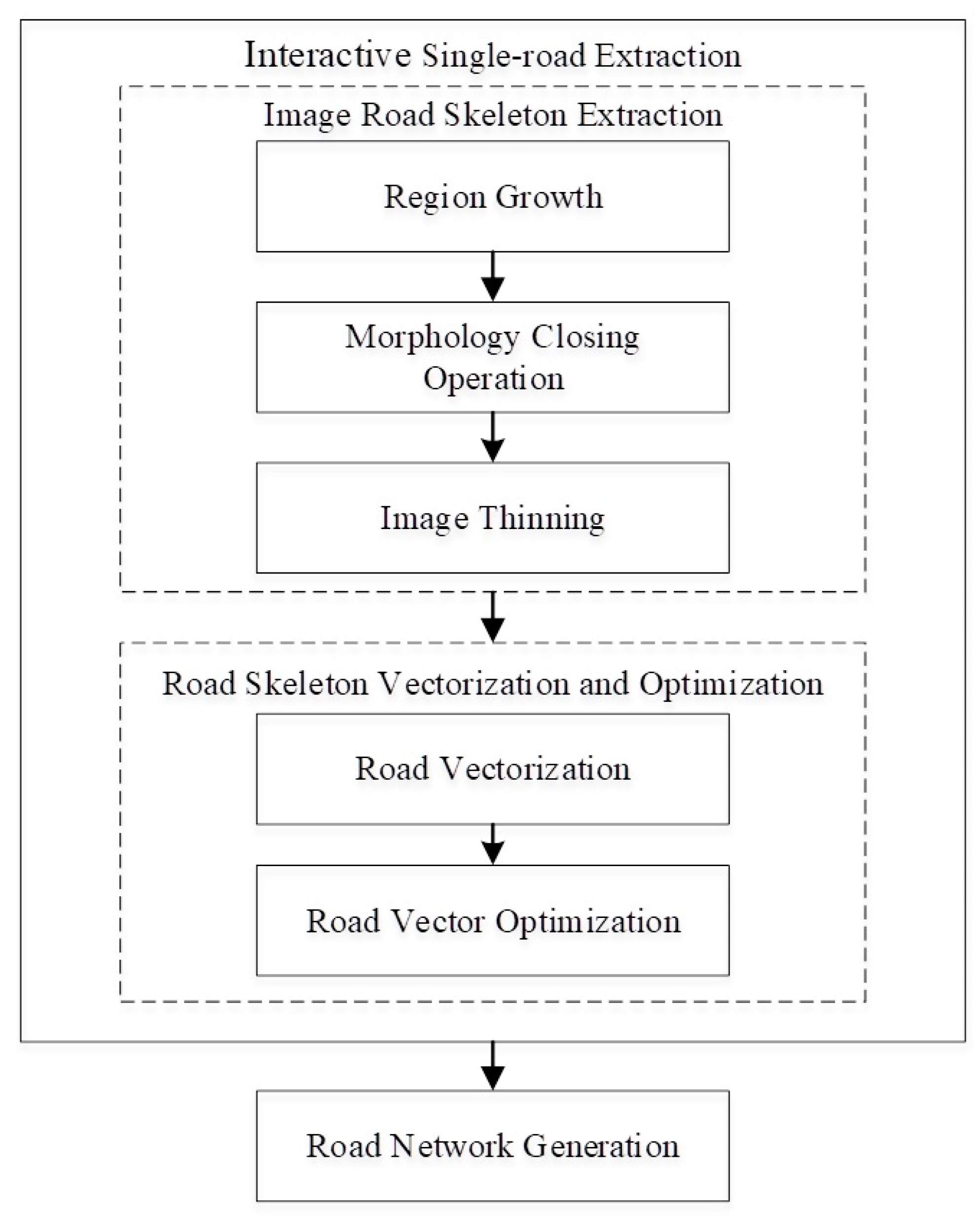
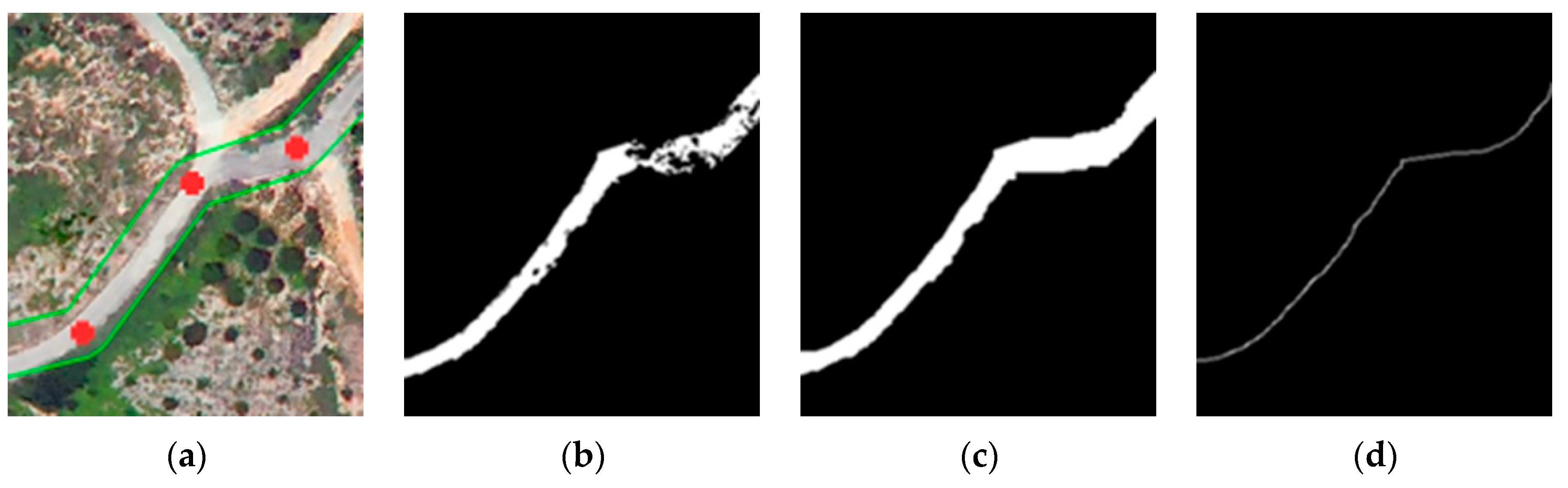
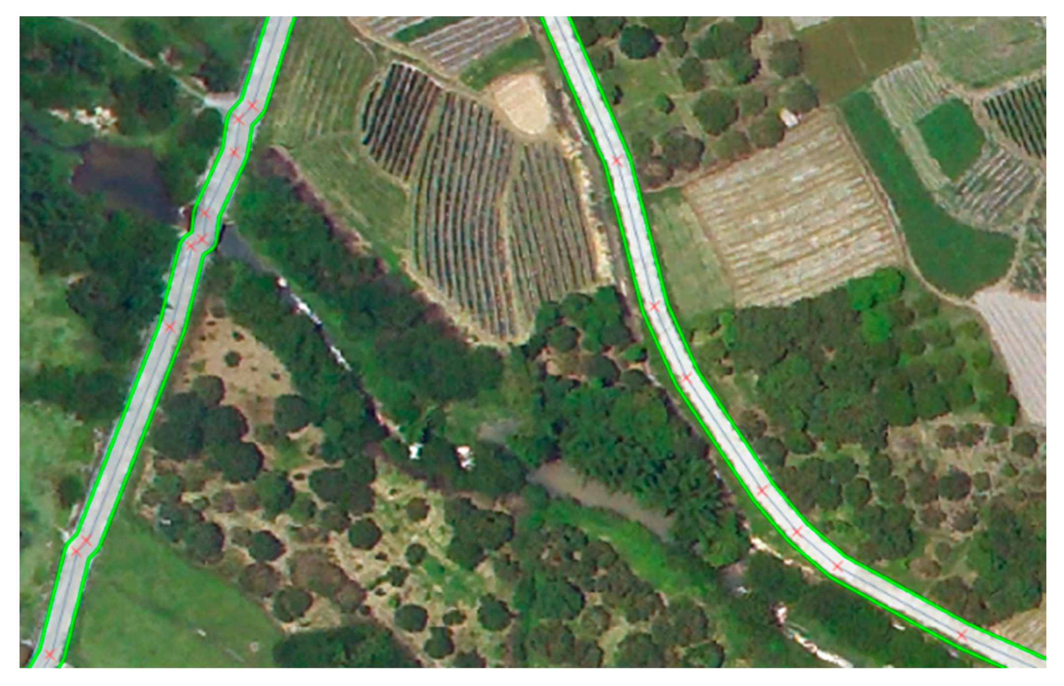
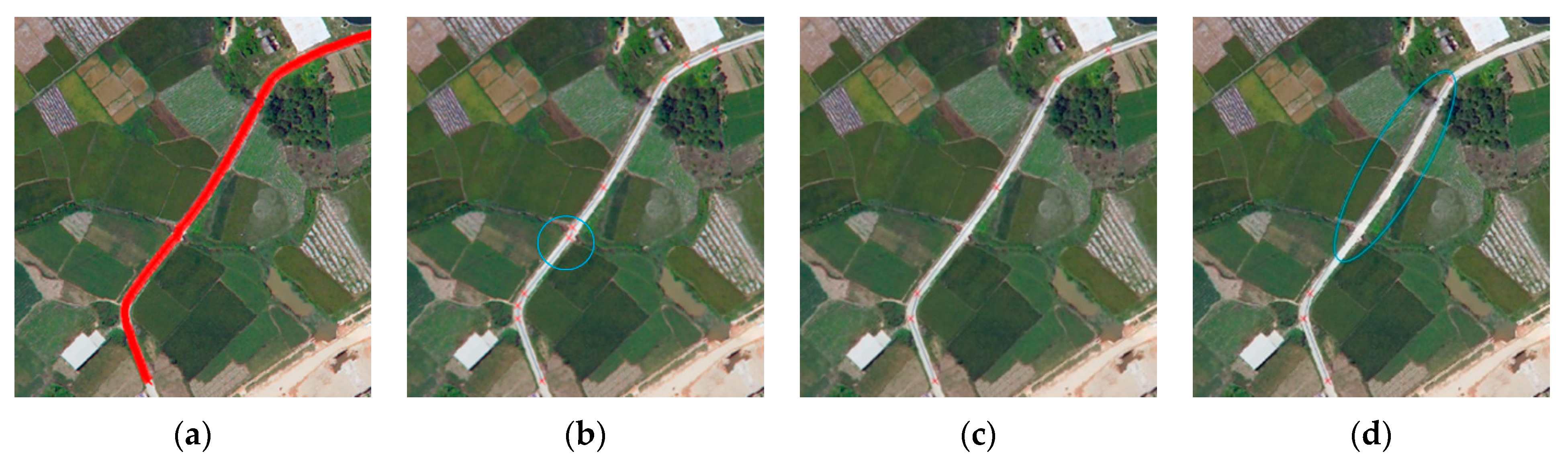
• A complete road network extraction framework with high accuracy and availability is proposed. With only a few seed points, the whole road can be obtained quickly. First, the width and seed points of a road are set interactively, and the skeleton of the road is extracted by using regional growth and morphological algorithms. Then, a single-road vector is obtained after vector tracking, vector simplification, endpoint modification, and road connection. Finally, the road network is generated by using intersection connection and buffer algorithms.
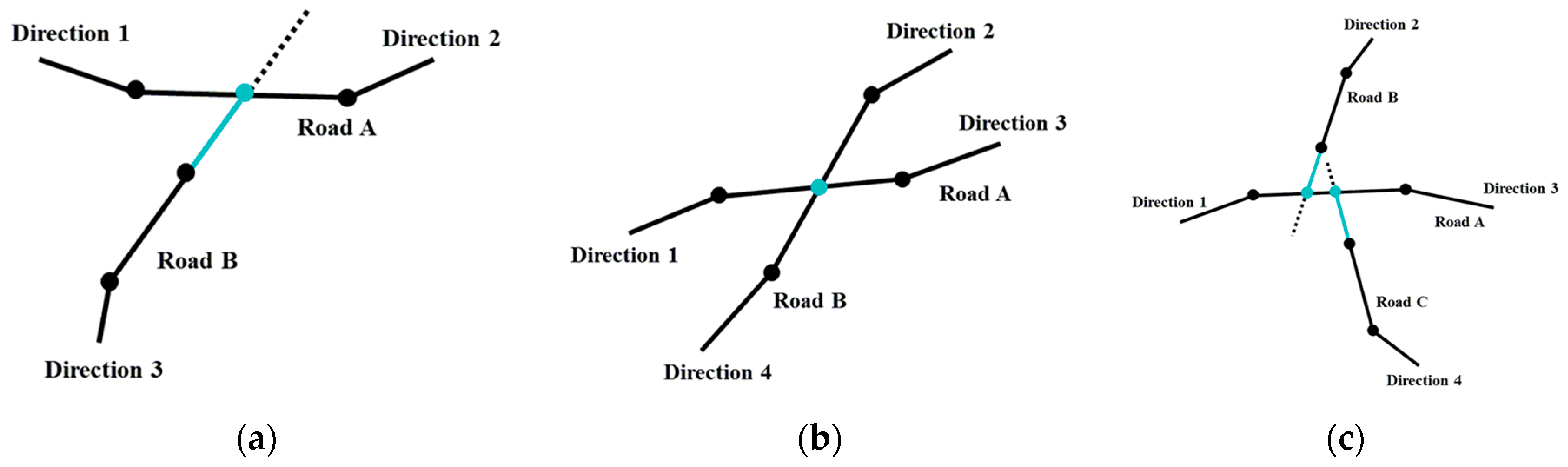
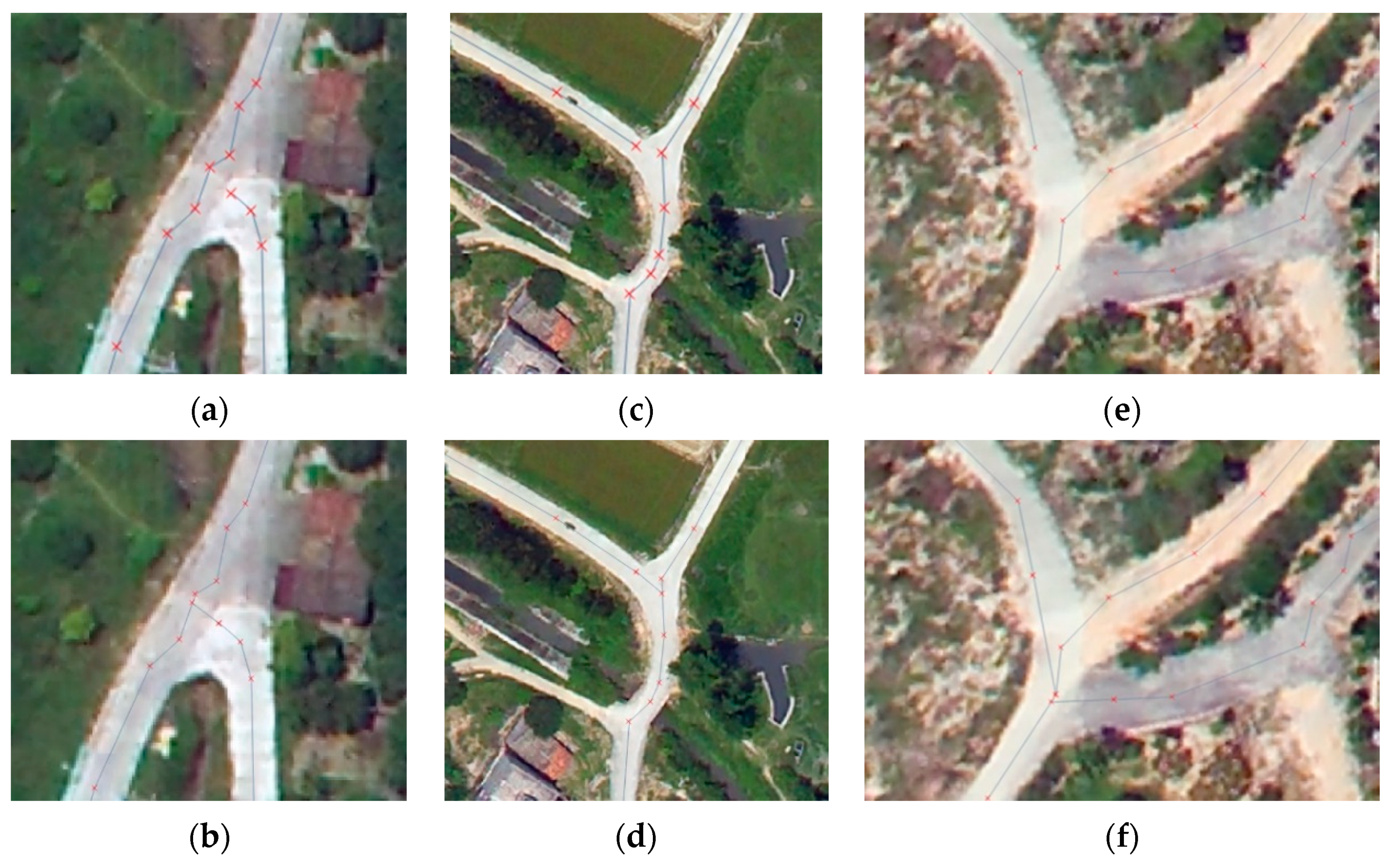
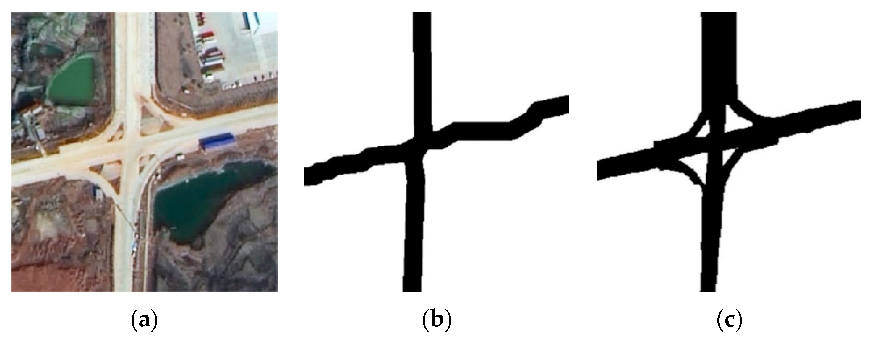
• To further improve the effectiveness of the proposed method, we adopt the road segment modification and road network construction strategy using the combination of grid image level and vector level. At the raster level, morphological algorithms are used to acquire the initial road segment, and at the vector level, further corrections and connections are completed based on road geometric features. For example, considering the ‘T’, ‘Y’, and ‘+’ shape of the intersection, an intersection connection algorithm is proposed.
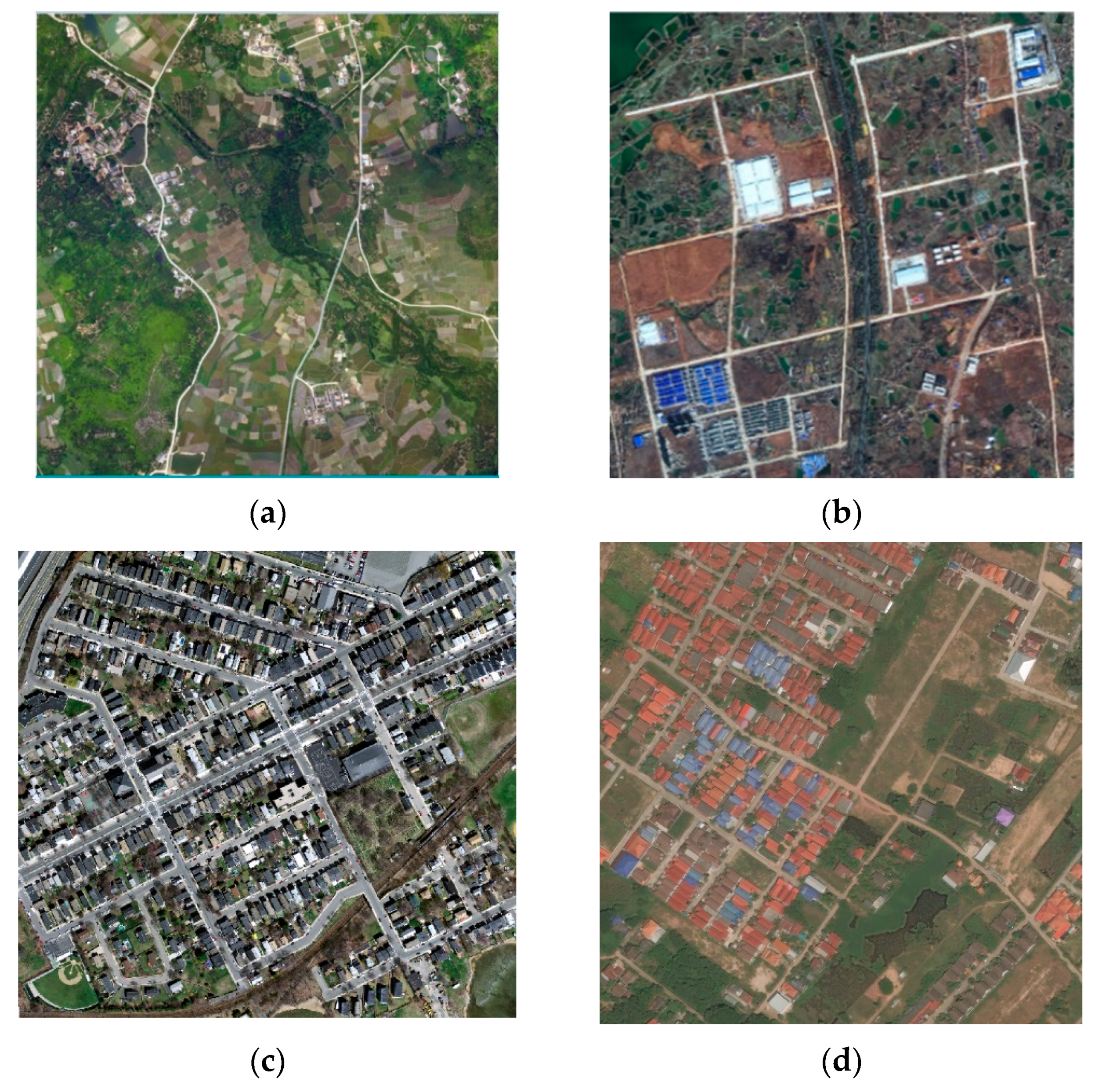
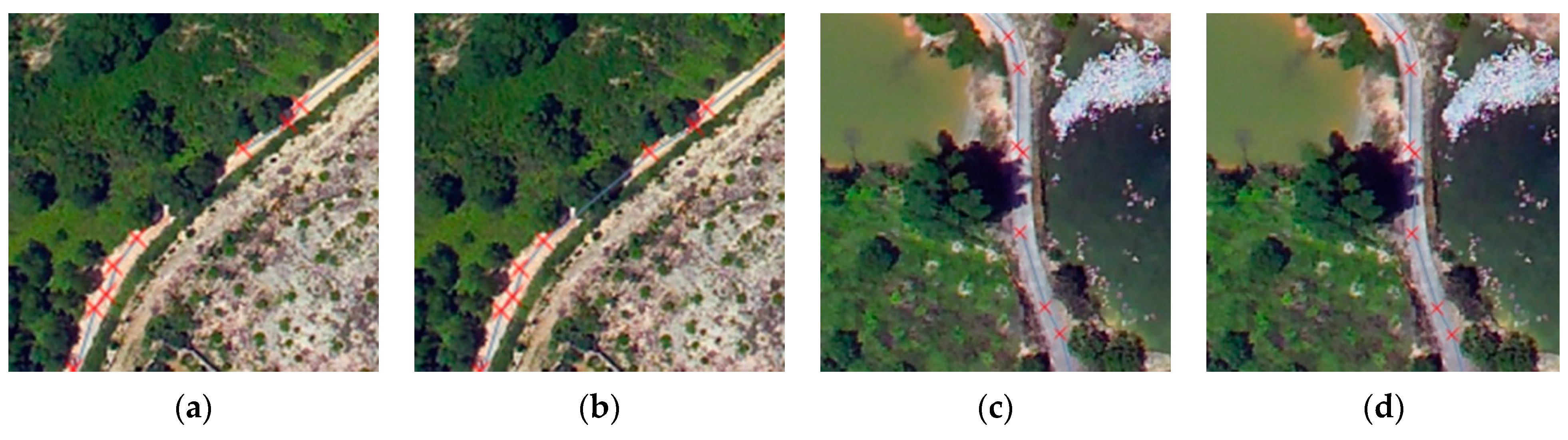
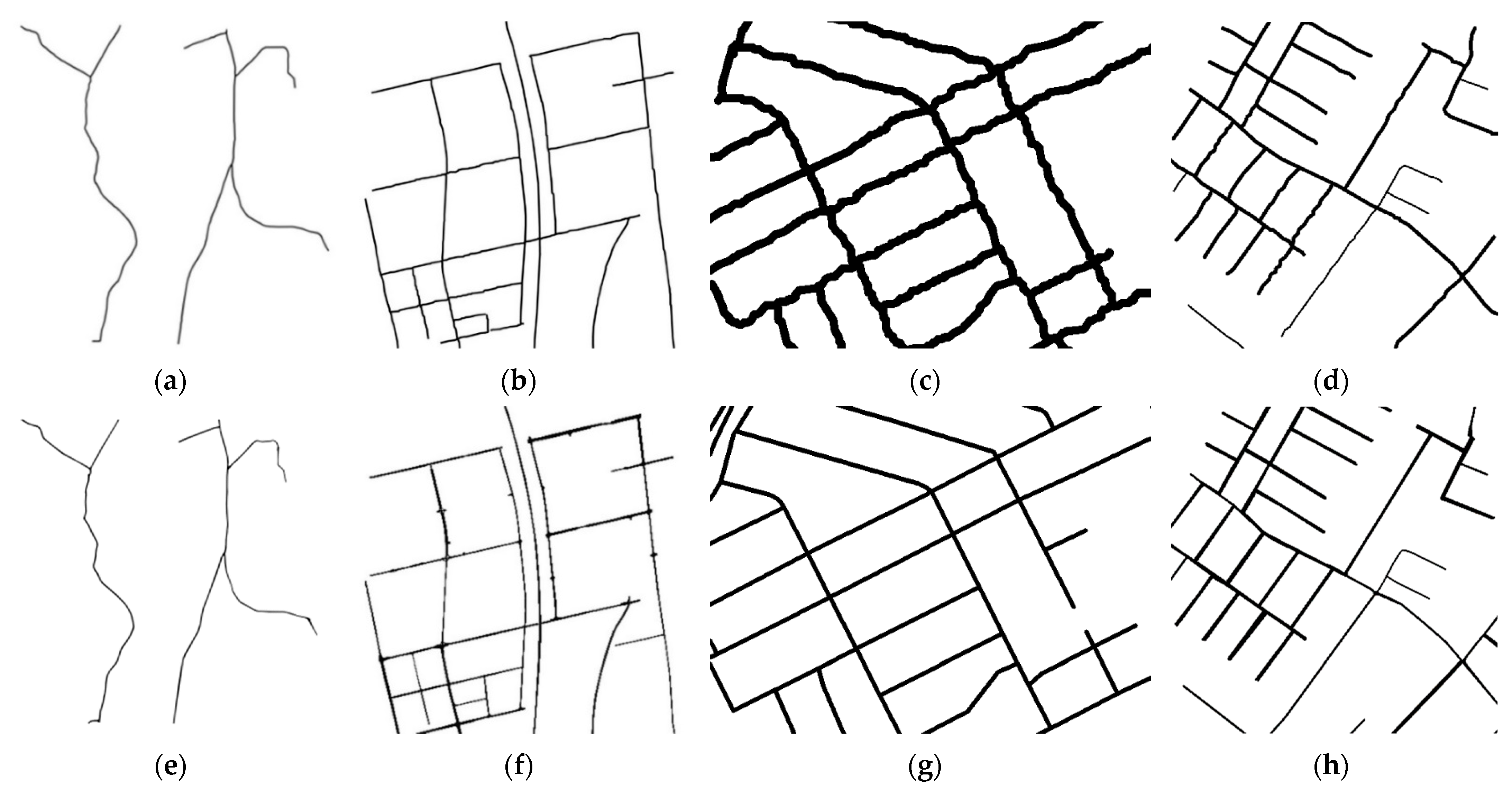
• The strategy proposed in this paper can be successfully applied to the extraction of rural areas, suburbs, and urban areas. At the same time, it also has a certain degree of correction effect on occlusion and shadow problems. The algorithm for extracting a single road can extract roads with a length of more than 4000 pixels at a time, which is fast and convenient, and has great potential for the application of labeling images for deep learning.

2. Materials and Methods

2.1. Experimental Data

Four different types of remote-sensing images were selected for road extraction experiments. One type is aerial images with a spatial resolution of 0.2 m of a certain rural area in Huizhou, Guangdong Province, as shown in Figure 1a, an image with a size of 5000 pixels × 5000 pixels is selected and recorded as Data 1. The second type is GF-2 satellite images with a spatial resolution of 1 m of a certain suburban district in Wuhan, Hubei Province, as shown in Figure 1b, an image with the same size as Data 1 is selected and recorded as Data 2. The third type is a partial image of the Massachusetts Road Data Set [45], with a size of 630 pixels × 600 pixels and spatial resolution of 1 m, which is recorded as Data 3 and shown in Figure 1c. For this image, a part of the image containing the road was left, and more details of the road can be seen by zooming in. The last image is one image in DeepGlobe Datasets [46], with a size of 1024 pixels × 1024 pixels and a spatial resolution of 0.5 m, which is recorded as Data 4 and shown in Figure 1d. Data 1 has only 6 long roads and 4 simple intersections but at least 8 obvious occlusions on the roads. Data 2 includes 21 roads and 26 different intersections, together with 14 areas of buildings. Additionally, there are more than 15 roads and 20 intersections in Data 3 and Data 4, with many buildings on the roadside.

2.2. Methodology

In remote-sensing images, roads have obvious shape characteristics, including high aspect ratio, small width changes, small curvatures, and ‘T’-, ‘Y’-, and ‘+’-shaped intersections, etc. The radiation characteristics of the roads are also obvious, such as consistent gray values, obvious edges, and uniform textures, etc. As shown in Figure 2, based on the characteristics of the road, the road network extraction method is composed of two parts: interactive single-road extraction and road network generation.

Single-road extraction is performed in four steps. First, a single growing point on the road is selected manually to acquire the road width automatically. Several seed points are further selected and a working area of the algorithm is generated at the same time according to the road width. Second, the skeleton of the road is obtained by region growth, morphological closing operations, and image thinning. Third, a tracking algorithm is used to vectorize the skeleton. Then, the optimized road segments are obtained through simplification and deletion of overly short segments. Finally, the endpoint modifications and road connections are processed to optimize the road segments further, and the broken road segments are connected into a complete road vector.

After obtaining a series of road vectors one by one, the road network generation algorithm is performed. First, complete vectorized centerlines are generated by intersection connection. After that, the road network is formed through the buffer algorithm.

2.2.1. Interactive Single-Road Extraction

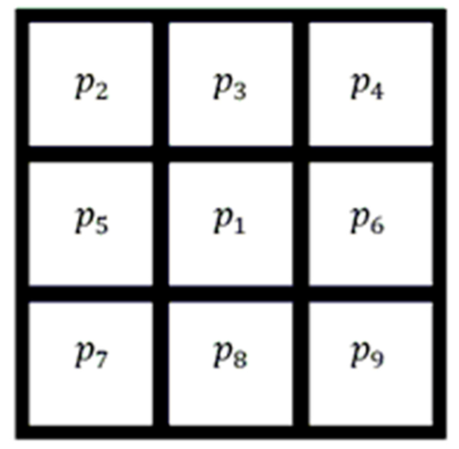
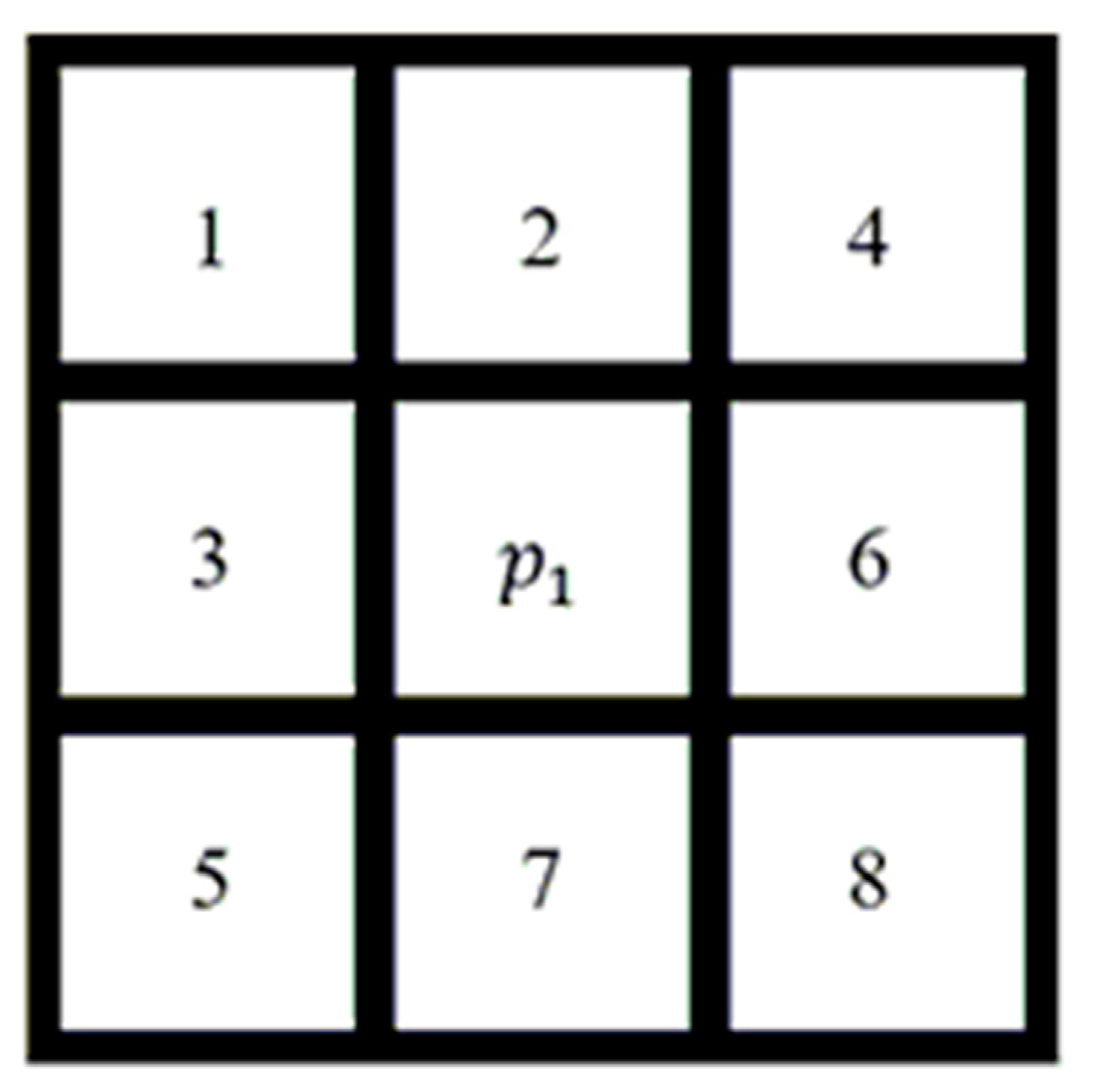
Image Road Skeleton Extraction

To obtain a complete road skeleton from high-resolution images, considering the glitches, holes, and interruptions that may be encountered during the extraction process, we use regional growth, morphological closing operations, and thinning algorithms to extract roads. To improve the accuracy and efficiency of road extraction, the spectral and geometric characteristics of roads are considered. We determine the implementation area of the algorithm according to the road width, thereby avoiding the problem of excessive growth.

For the purpose of obtaining the road width, we first perform regional growth in a local area to obtain one segment with parallel edges. The operation of regional growth can be described as follows: first, select a certain pixel on the road as the growing point. Especially, for road width determination, the growing point should be located on a road segment without glitches, holes, or interruptions. Next, compare the grayscale of the growing point with its eight neighborhoods. Finally, combine the neighbor pixels meeting the merge threshold requirements with growing point and set it as a new growing point until no new pixels are combined. Regional growth has a simple rule, high calculating speed and interactivity, which is suitable for road extraction requirements. The road width L is defined in meters by calculating the minimum distance between the edges of the local road segment.

Then, several seed points are selected manually on the road from one end to the other, and a working area of the regional growth algorithm is limited by a buffer algorithm with the line of seed points as the central axis. When selecting seed points, we only need to ensure that the working area can cover the whole road. As shown in Figure 3a, the seed points are in red and the green border delineates the working area. Then, the operations of regional growth and morphological processing are performed in the working area.

To extract one long road at a time, we use the strategy of growing multiple seed points simultaneously. This method has the advantages of simple rules and a high calculation speed. The regional growth results are shown in Figure 3b, and a relatively complete road can be extracted. However, there are burrs and rough areas on the edges of the generated roads due to the pixel-by-pixel processing of the regional growth algorithm; there are also many holes inside the road, which are caused by incomplete growth due to shadows, occlusions, etc. Therefore, further optimization of the regional growth results is needed. To minimize the errors of holes and fragmented growth, this method adopts the morphological closing operation, which is most commonly used for trimming edges and filling gaps, to optimize the initial extraction results. The morphological closing operation [12] is defined as follows:

$$\mathrm{A}·\mathrm{B}=\left(\mathrm{A}\oplus \mathrm{B}\right)\ominus \mathrm{B},$$

(1)

In the formula, the operator ∙ denotes the closing operation, A represents the binary image, and B represents the structural elements. The symbols $\oplus$ and ⊖ denote the expansion and corrosion operators, respectively. Figure 3c shows the result of the morphological closing operation.

The road skeleton is the basis for generating the road network. Therefore, we use a morphological thinning algorithm to skeletonize the previously extracted roads. By progressively stripping the road pixels, only a single-pixel-width skeleton is left to maintain connectivity. The Zhang–Suen parallel algorithm [47] is used for refinement. Because of its low number of iterations and high speed, it has superior thinning ability at intersections and is widely used in the field of image thinning [3,12,48]. By searching the points of roads one by one in the binary image obtained by the morphological closing operation, where a road point has a gray value of 255 and a background point has a value of 0, boundary points that do not affect road connectivity are deleted. The operation has two steps:

Step 1: Find the boundary points that meet the following requirements:

$$2\le {\mathrm{N}}_1\le 6,$$

(2)

$$\mathrm{T}\left({\mathrm{p}}_1\right)=1,$$

(3)

In the formulas, ${\mathrm{N}}_1$ means the number of road points among eight neighborhoods, and $\mathrm{T}\left({\mathrm{p}}_1\right)$ is the number of transitions of gray values from 0 to 255 among eight neighborhoods.

Step 2: if a boundary point found meets requirements of either group A or group B, its gray value will be changed to 0, which means it is deleted. In the formulas, ${\mathrm{p}}_{\mathrm{i}}$ means the gray value of the i-th pixel. The arrangement of pixels is shown in Figure 4.

Group A:

$${\mathrm{p}}_2·{\mathrm{p}}_4·{\mathrm{p}}_6=0,$$

(4)

$${\mathrm{p}}_4·{\mathrm{p}}_6·{\mathrm{p}}_8=0,$$

(5)

Group B:

$${\mathrm{p}}_2·{\mathrm{p}}_4·{\mathrm{p}}_8=0,$$

(6)

$${\mathrm{p}}_2·{\mathrm{p}}_6·{\mathrm{p}}_8=0,$$

(7)

Repeat the two steps until no more points should be deleted. The result is shown in Figure 3d.

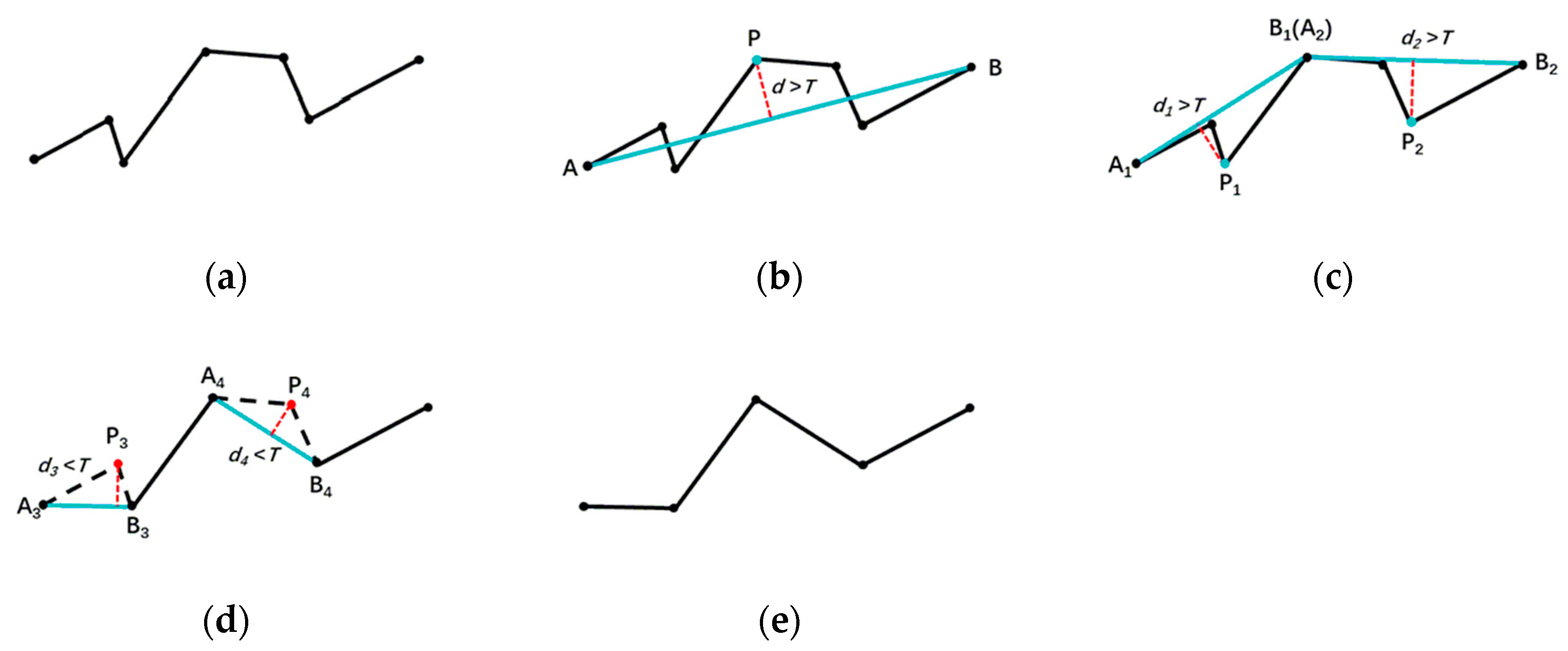
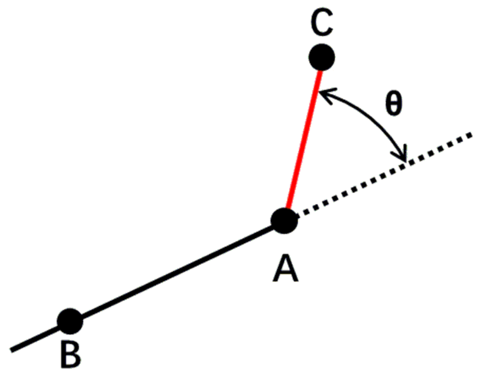
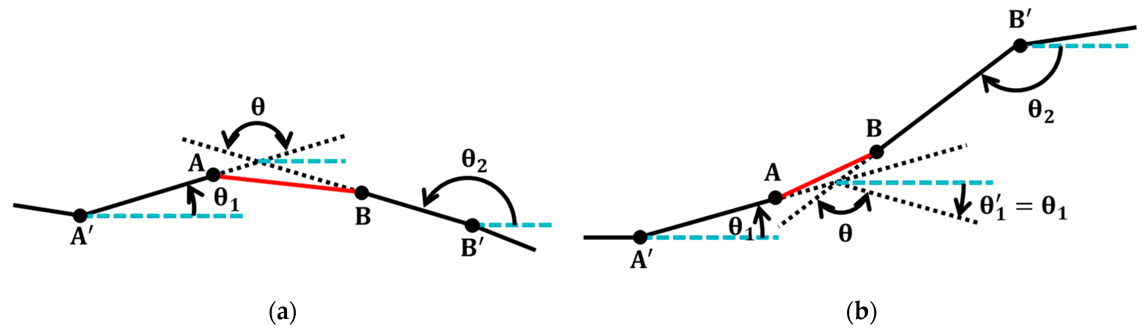
Road Skeleton Vectorization and Optimization

After the processing described above, a road skeleton with a single-pixel width is acquired. Compared with the raster map, the vector map is more convenient to save and modify and easier to update and use in data analysis. Therefore, it is necessary to perform vectorization processing on the road skeleton obtained. We use a tracking algorithm to vectorize the road skeleton. To obtain a relatively accurate centerline vector of the road and address the problems of overly short segments and incomplete roads, various operations are adopted, which include simplifying road segments, deleting overly short segments, modifying endpoints, and connecting roads. The strategies and algorithms used in each part are introduced below.

(1)

Road vectorization to generate road segments

This method uses a road tracking algorithm to vectorize the raster road; the results of this algorithm are accurate, and its calculation speed is high. This operation can be described as the following steps:

Step 1: Search for a starting road point (with a gray value of 255, pixel ${\mathrm{p}}_1$ in Figure 4) in the whole image from top left to bottom right and record its coordinate, then record this point as the first point of a road and change its gray value to 0, that is, delete it.

Step 2: search for another road point in a certain order (see Figure 5) in the eight neighborhoods of the first point and set it as a new starting point. Then record this point as the latter point of the road and also change its gray value to 0. Repeat this step until no more road points are to be recorded.

Step 3: As the first point may not be the actual starting point of a road, set the first point as the starting point again and continue searching in the same order as step 2, but record the new point found as a previous point instead, indicating that the road being tracked has a certain direction.

Step 4: When no new points needs to be recorded in step 3, an entire road has been recorded and all the points of it have been deleted. Start again from step 1 to track a new road and stop tracking when no road points can be found in the entire image.

The simplifying algorithm and the operation of deleting overly short segments are applied after the tracking algorithm. We use the Douglas–Peucker algorithm [49] for simplification; it has translation and rotation invariance and removes unnecessary points by setting a distance threshold to perform data compression. This algorithm mainly includes these following steps:

Step 1: Connect the two endpoints A and B and record them as reserved points. Calculate the Euclidean distance from each point between the two ends to line $\overline{\mathrm{AB}}$, and find the point P with the greatest distance. If there is no point between the two ends, all points have been simplified, and the simplifying operation exits.

Step 2: Compare the distance from point P to line $\overline{\mathrm{AB}}$ and the simplifying threshold T, delete point P when the distance is less than T, otherwise, keep it.

Step 3: Repeat the steps above with points A and P as endpoints and with B and P as endpoints, respectively.

The simplifying threshold T is defined as:

$$\mathrm{T}=\mathrm{k}\times \mathrm{resolution},$$

(8)

where resolution is the image resolution in meters; k is a simplifying parameter, which is set to 3.0.

Figure 6 shows the principle of the Douglas–Peucker algorithm: the endpoints are determined and deleted in turn, and finally a five-point polyline is used to describe the initial seven-point polyline. Blue points are the ones being judged and then kept, and the red points are the ones judged and then deleted. Red dashed lines show the distances between the judged point P and the connecting line of endpoints A and B (blue line) and black dashed lines are the segments to be deleted in each step.

During the road tracking process, due to the influence of intersections, shadows, etc., on the road, some overly short segments may be generated, as shown in Figure 7a,b. These overly short segments are not part of the road and are likely to cause interference in the subsequent connection algorithms. Therefore, we delete them by setting a length threshold. The length threshold ${\mathrm{d}}_{\mathrm{t}}$ is defined as:

$${\mathrm{d}}_{\mathrm{t}}=10\times \mathrm{L},$$

(9)

This definition is based on the characteristics of long and thin roads; according to experience, the aspect ratio of roads is generally greater than 10.

The road vectorization algorithm is shown in Algorithm 1:

Algorithm 1: Road Vectorization
Input: image Input Image             neighbor Neighborhood Search Order             dt Length Threshold Output: Lines Segments
1:	function FindLines(image, Lines, neighbor, dt)
2:	BEGIN
3:	while (findFirstPoint(image, firstPt))
4:	BEGIN
5:	line.push_back(firstPt);
6:	currPt = firstPt;
7:	while (findNextPoint(neighbor, image, currPt, nextPt))
8:	BEGIN
9:	line.push_back(nextPt);
10:	currPt = nextPt;
11:	END
12:	currPt = firstPt;
13:	while (findNextPoint(neighbor, image, currPt, nextPt))
14:	BEGIN
15:	line.push_front(nextPt);
16:	currPt = nextPt;
17:	END
18:	if (line.length() > dt)
19:	BEGIN
20:	line.simplify(T);
21:	Lines.push_back(line);
22:	END
23:	END
24:	END

Among the functions above, findFirstPoint (image, firstPt) is used to globally search for the first point firstPt, findNextPoint (neighbor, image, currPt, nextPt) is used to search for the next point nextPt, and line.simplify (T) is used to simplify the line segment according to the threshold T.

Figure 7 shows the result of vectorization processing: (a) is a local road thinning result, (b) shows the road segments obtained by the tracking algorithm, (c) is the result of deleting overly short segments, and (d) is the result of the simplifying algorithm.

(2)

Road segment optimization and connection

The vectorization operation mentioned above generates a series of separate road segments, and the offset problem occurring at the head and tail segments during the thinning process cannot be solved, as shown in Figure 8a,c. Therefore, the road segments generated need to be further optimized and connected to form the entire road.

Considering the smoothness of roads, branches and offsets are eliminated by judging the direction of the endpoints and the neighboring nodes. The principle of endpoint modification is shown in Figure 9, where the dotted line indicates the direction of vector $\overline{\mathrm{BA}}$. For each segment, two consecutive nodes $\mathrm{A}$ and $\mathrm{B}$ adjacent to endpoint $\mathrm{C}$ are selected, and $\mathsf{\theta }$ is the angle between the vectors $\overline{\mathrm{BA}}$ and $\overline{\mathrm{AC}}$. Endpoint $\mathrm{C}$ is retained when $\mathsf{\theta }<10°$. Otherwise, it is deleted along with the overly short segment, shown in red in Figure 9. Figure 8b,d show the results of road segment optimization.

To connect the optimized segments into an entire road, a road connection algorithm is designed. The connection rules include rules governing the distance between endpoints and the angle between vectors. If two segments meet the connection rules, the endpoints are connected.

The rule governing the distance between endpoints is defined as follows: first, the distance between two endpoints must be the shortest globally. Second, considering the continuous and uninterrupted characteristics of a road, we again choose ${\mathrm{d}}_{\mathrm{t}}$ as the distance threshold for connection. The distance between two connected endpoints should be less than ${\mathrm{d}}_{\mathrm{t}}$.

Furthermore, considering the smoothness of a specific road, the rule governing the angle between vectors is defined as shown in Figure 10. Black solid lines show the segments, black dotted lines show their extensions, and blue dashed lines indicate the horizontal-right direction. If the endpoints A and B of the road segment meet the distance rule, then we find the nodes A′ and B′ adjacent to the endpoints A and B. ${\mathsf{\theta }}_1$ and ${\mathsf{\theta }}_2 \left({\mathsf{\theta }}_1,{\mathsf{\theta }}_2\in \left(0°,180°\right]\right)$ are the angles between the vectors $\overrightarrow{\mathrm{A}’\mathrm{A}}$ and $\overrightarrow{\mathrm{B}’\mathrm{B}}$ and the horizontal-right direction, respectively, and $\mathsf{\theta }=\left|{\mathsf{\theta }}_1-{\mathsf{\theta }}_2\right|$. If $\mathsf{\theta }>90°$, the endpoints are connected. The connection line is shown in red.

The pseudocode of the road connection algorithm in Algorithm 2:

Algorithm 2: Road Connection
Input:   Lines Segments after Tracking Algorithm Output: Lines Roads after Connection Algorithm
1:	function LinkLines(&Lines)
2:	BEGIN
3:	Ver = FindVertex(Lines);
4:	Ver_theta = FindVertexAzimuth(Lines);
5:	for i ← 0 to Ver.size()
6:	BEGIN
7:	min = 9999.0;
8:	if (isinConnectedPt(i, ConnectedPt)) continue;
9:	for j ← (i + 1) to Ver.size()
10:	BEGIN
11:	if (isinSameLine(Ver(i), Ver(j))) continue;
12:	temp_distance = cal_Distance(Ver(i),Ver(j));
13:	if (temp_distance < min)
14:	BEGIN
15:	min = temp_distance;
16:	flag = j;
17:	END
18:	END
19:	if ((abs(Ver_theta(i)-Ver_theta(flag)) > 90) AND (min < dt))
20:	BEGIN
21:	Temp_line.pushback(Ver(i));
22:	Temp_line.pushback(Ver(flag));
23:	L1 = findLinefromVer(Ver(i));
24:	L2 = findLinefromVer(Ver(flag));
25:	JudgeConnectOrder(L1,L2,&Line1,Temp_line,&Line2);
26:	Line1 = Line1.combine(Temp_line);
27:	Line1 = Line1.combine(Line2);
28:	ChangeLine(L1,Line1, &Lines);
29:	deleteLine(L2,&Lines);
30:	ConnectedPt.pushback(flag);
31:	END
32:	END
33:	END

FindVertex (Lines) is used to find the endpoint of the segment. FindVertexAzimuth (Lines) is used to calculate the angle between the end vector and the horizontal-right direction. ConnectedPt stores the number of connected vertices. The isinConnectedPt(i, connectedpt) function is used to determine whether the currently numbered vertex i has been connected; isinSameLine(Ver(i), Ver(j)) is used to judge whether the two vertices are on the same road segment; cal_Distance(Ver(i), Ver(j)) is used to calculate the Euclidean distance between two vertices; findLinefromVer(Ver(i)) is used to find the corresponding road segment through vertex Ver(i); and JudgeConnectOrder(L1, L2, & Line1, Temp_line, & Line2) is used to determine the connection order. The combine function connects segments. ChangeLine(L1, Line1, & Lines) is used to reset lines and deleteLine(L2, & Lines) is used to delete redundant segments.

Figure 11 shows the connection results of single roads, in which (a) and (c) depict two roads to be connected. The middle part of each road is divided into two sections due to tree occlusion, and this cannot be repaired by the morphological closing algorithm; (b) and (d) show the road connection results.

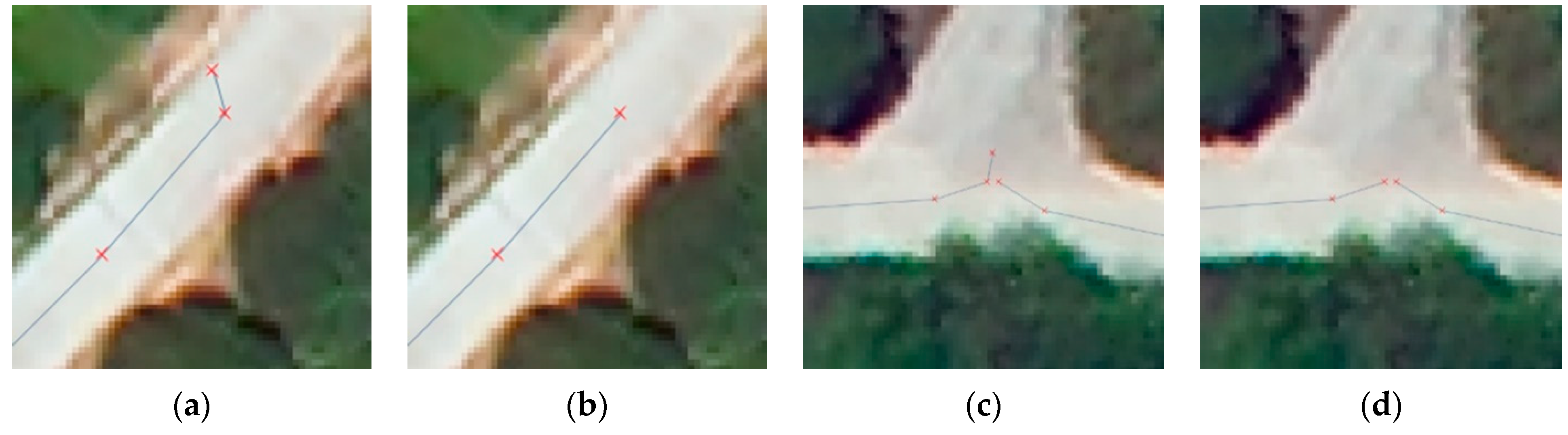
2.2.2. Road Network Generation

The road network is acquired through road intersection connections and buffer generation. Road intersections have three main shape types: ‘T’, ‘Y’, and ‘+’. ‘T’- and ‘Y’-shaped intersections are similar, as shown in Figure 12a, in which directions 1 and 2 with larger included angles can be regarded as the same single road, recorded as road A. Direction 3 is regarded as a single road and is recorded as road B. At this time, the extension line (dashed line) of road B is constructed to a certain length, which is equal to ${\mathrm{d}}_{\mathrm{t}}$, to determine whether there is an intersection with road A. If an intersection exists (blue point), it is connected to road B (blue line).

There are two situations for an intersection with a ‘+’ shape. One is shown in Figure 12b. The four directions intersect at the same point, and the angles between directions 1 and 3 and between 2 and 4 are both close to 180°; this can be taken to indicate two single roads that should be extracted separately, and the roads A and B obtained have a unique intersection (blue point). No additional processing is required. The other situation is relatively complicated, as shown in Figure 12c. Directions 1 and 3 can be regarded as the same road for extraction to obtain road A, while directions 2 and 4 can only be extracted as individual roads that generate roads B and C. In this case, the intersection can be regarded as the superposition of two ‘T’-shaped roads formed by road A with either B or C. Then, processing can be performed according to the ‘T’-shaped intersection connection strategy.

Figure 13 shows the connection results of the intersection connection algorithm. It can be seen that the strategy described above has a good connection effect.

The intersection connection algorithm is shown in Algorithm 3:

Algorithm 3: Intersection Connection
Input:    Lines Roads Output: addLines Newly added connection roads
1:	function addJunctionLines(Lines, addLines)
2:	BEGIN
3:	Ver = FindVertex(Lines);
4:	Ver_theta = FindVertexAzimuth(Lines);
5:	for i ← 0 to Ver.size()
6:	BEGIN
7:	extendline.push_back(Ver(i));
8:	extendpoint = cal_coordinate(Ver(i), Ver_theta(i), dt);
9:	extendline.push_back(extendpoint);
10:	for j ← 0 to Lines.size()
11:	BEGIN
12:	if (intersects(Lines(j), extendline))
13:	BEGIN
14:	intersect_geo = intersection(Lines(j), extendline);
15:	intersect = intersect_geo- > asPoint();
16:	if (Ver(i)≠intersect)
17:	BEGIN
18:	temp_polyline.push_back(Ver(i));
19:	temp_polyline.push_back(intersect);
20:	addLines.pushback(temp_polyline);
21:	END
22:	END
23:	END
24:	END
25:	END

The function cal_coordinate(Ver(i), Ver_theta(i), dt) is used to calculate the vertex of the extension line of limited length; intersects(Lines (j), extendline) is used to determine whether there is an intersection; and intersection(Lines (j), extendline) is used to calculate the intersection.

After multiple roads are extracted separately and all road endpoints are judged and connected, a buffer zone with a radius that is one-half the width of the road is generated to obtain the road network (see Figure 14).

2.2.3. Evaluation of the Extraction Results

In this method, the precision, accuracy, recall, and intersection over union (IoU) [50,51] are used to evaluate extraction performance, see Equations (10)–(14). In the formulas, TP, FP, FN, and TN are the number of true positives, false positives, false negatives, and true negatives for the road predictions.

$$\mathrm{Precision}=\frac{\mathrm{TP}}{\mathrm{TP}+\mathrm{FP}} ,$$

(10)

$$\mathrm{Accuracy}=\frac{\mathrm{TP}+\mathrm{TN}}{\mathrm{TP}+\mathrm{TN}+\mathrm{FP}+\mathrm{FN}} ,$$

(11)

$$\mathrm{Recall}=\frac{\mathrm{TP}}{\mathrm{TP}+\mathrm{FN}} ,$$

(12)

The IoU is the ratio of the intersection and the union of two bounding boxes. If A is the resulting extracted road and B is the corresponding ground truth, then the IoU is:

$$\mathrm{IoU}=\frac{\mathrm{A}\cap \mathrm{B}}{\mathrm{A}\cup \mathrm{B}} ,$$

(13)

TP, FP, and FN are used to re-state the formula as follows:

If the extraction result is identical to the ground truth, then IoU is equal to 1.

$$\mathrm{IoU}=\frac{\mathrm{TP}}{\mathrm{TP}+\mathrm{FN}+\mathrm{FP}} ,$$

(14)

3. Results

3.1. Parameter Settings

In this study, only three parameters need to be set in the workflow of road network extraction: the image resolution, regional growth threshold, and simplifying threshold. The image resolution can be obtained directly from the data source. Since the difference in gray value between urban buildings and roads is small, the regional growth threshold needs to be determined by the user according to the number of buildings shown in the image. After a large number of experiments, the regional growth threshold was set to 40 in suburbs with fewer buildings, and 20 in cities with more buildings. As shown in Equation (8), the simplifying parameter $\mathrm{k}$ has a significant impact on the simplified result. Based on experiments, the simplifying parameter k is set to 3. Figure 15 shows the results of different simplifying thresholds for an image with the same type as Data 2; (a) is the tracking result, and (b–d) are the simplified results when the simplifying parameter k is 1, 3, and 5, respectively. When k = 1, redundant points remain in the circle. When k = 5, some key points are missing, and the centerline in the circle deviates from the road. When k = 3, the result fits the road centerline well. Hence, the simplifying parameter k is set to 3 here.

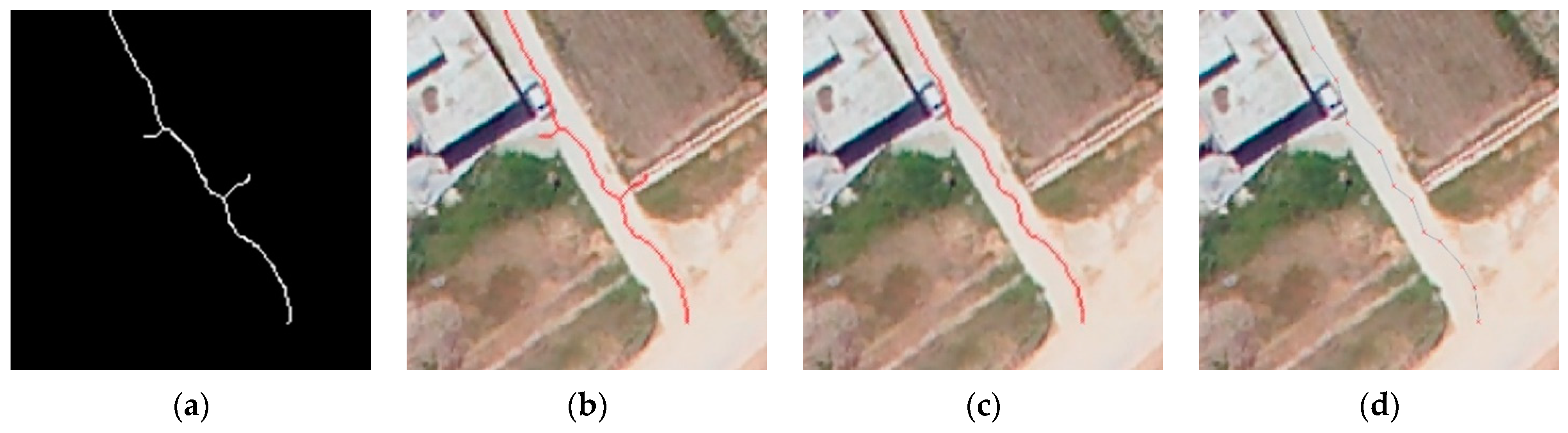
3.2. Road Extraction Results for the Four Datasets

Figure 16 shows a comparison between the road extraction result and the ground truth, where (a,e) correspond to Data 1, (b,f) correspond to Data 2, (c,g) correspond to Data 3, and (d,h) correspond to Data 4; (a–d) are extracted by the developed method to generate road networks, and (e–h) are ground truths that are manually labeled. The evaluation results are shown in

Table 1. Evaluation table of road extraction.

Data	Precision	Accuracy	Recall	IoU
Data 1	88.54%	99.70%	88.97%	0.80
Data 2	87.08%	98.13%	77.06%	0.69
Data 3	98.10%	88.31%	88.68%	0.87
Data 4	80.70%	96.80%	81.56%	0.68

. These extraction results have high accuracy and precision of Data 1–3, showing that the method applies well in extracting roads from images at different resolutions. Among the four data, Data 1 was located in a rural area, with the simplest road conditions and the highest resolution. Therefore, the extraction result is very similar to the ground truth (Figure 16a,e). Data 2 is more complex than Data 1, but each road is also extracted relatively completely (Figure 16b,f). Because of many details in Data 2, the recall rate and IoU in the road extraction results are relatively low (Table 1). Data 3 is located in the city, and the road situation is the most complex. The results of Data 3 have the highest precision but the lowest accuracy (Table 1), meaning that most parts of roads are identified accurately but the differences between roads and surroundings are not distinguished well. Data 4 is located in a rural residential area with multiple roads of varying lengths and widths. The proposed method can extract the roads in the image very well by extracting the roads by grading, that is, firstly extracting the wide roads, and then extracting the narrow roads (Figure 16e,h). However, the width of the road at the same level in the image is also different, which makes the proposed method obtain limited extraction precision and IoU (Table 1). Moreover, all road intersections in the four data are correctly connected.

Ten roads in Data 2 were randomly selected for statistical analysis of extraction time (

Table 2. Evaluation table of road extraction efficiency.

No.	Road Length (pixel)	Time (s)	Time per 1000 pixels (s)
1	2040	4.125	2.02
2	2126	4.739	2.23
3	2378	4.64	1.95
4	2415	5.688	2.36
5	2770	6.776	2.45
6	4056	4.536	1.12
7	4064	6.43	1.58
8	4115	5.83	1.42
9	4121	6.095	1.48
10	4188	6.486	1.55
Mean	-	-	1.81

). Roads with a length of more than 4000 pixels can be extracted at one time in 7 s. In terms of extraction efficiency, the longer the road, the shorter the road extraction time per 1000 pixels. The average extraction time of roads per 1000 pixels is 1.81 s.

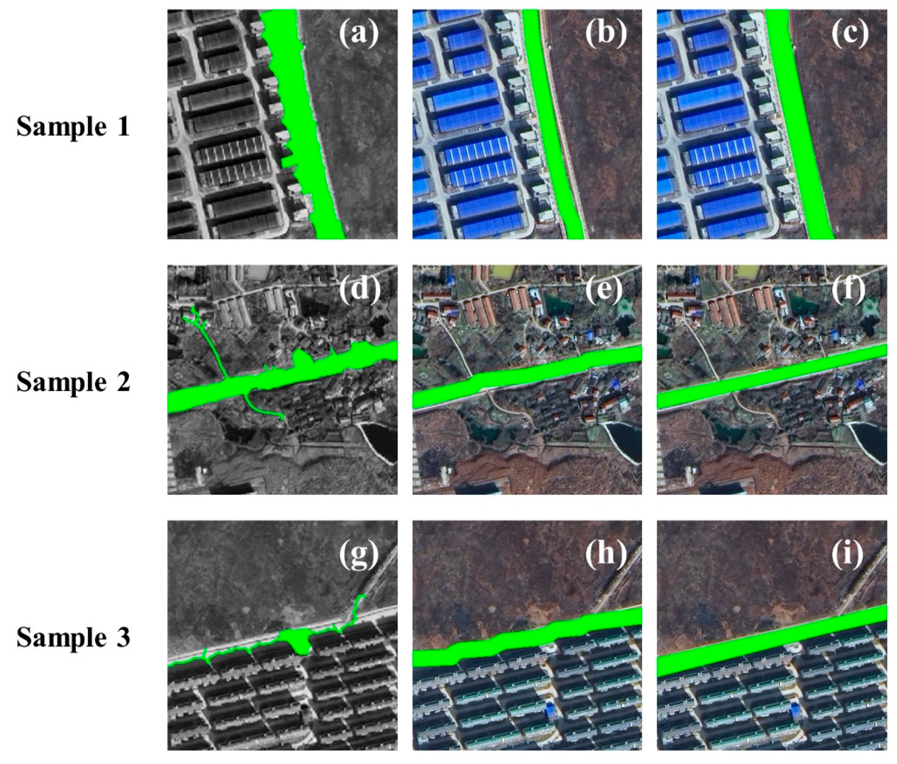
3.3. Comparison with Other Existing Methods

We make comparisons with Gu’s road extraction method [41] in this study. Gu’s method is implemented in the following way: first determine a seed point to obtain the initial contour through region growth (use the same threshold as the developed method), and then use the GVF–Snake method to perform iterative optimization to obtain the road boundary, where the number of iterations is 40. Gu’s method has many iterations, so it is only suitable for road extraction in local areas. Three local typical roads were selected for comparison. For each road segment about the length of 300 pixels, the method takes around 2 s. This is less efficient than the developed method (Table 2). Figure 16 shows the extraction results of the two methods.

For Sample 1 and Sample 2, the recall of Gu’s method is higher than ours. However, the precision and IoU of the developed method are all better than those of Gu’s method (

Table 3. Performance of local road extraction by Gu’s method and the proposed method.

	Sample 1		Sample 2		Sample 3
	Gu’s Method	Proposed Method	Gu’s Method	Proposed Method	Gu’s Method	Proposed Method
Precision	0.64	0.96	0.57	0.79	0.76	0.84
Accuracy	0.94	0.97	0.96	0.98	0.94	0.98
Recall	0.88	0.70	0.99	0.94	0.25	0.86
IoU	0.59	0.67	0.57	0.75	0.23	0.73

). As shown in Figure 17a,d, Gu’s method could distinguish wild country and artificial structures exposed to the sun, including roads, which led to high recall. However, it was easily influenced by the effect of ‘different objects with similar spectra’. Objects such as concrete ground and bare soil were extracted as roads, leading to low precision, accuracy, and IoU (Table 3). Because of the limited working area, the developed method could avoid over-extraction (Figure 17b,e) and thus reach better precision, accuracy, and IoU (Table 3). When shadows occlude some roads, such as those in Sample 3, Gu’s method could hardly identify these roads (Figure 16g), significantly reducing its recall and IoU (Table 3). In the developed method, roads were thinned to centerlines and regenerated with a certain width, which weakened the influence of shadows (Figure 17h) and achieved an acceptable result (Table 3). Furthermore, the series of operations including morphological operation and vector simplification in the developed method eliminated the burs and made the road edge smoother.

4. Discussion

After applying the method in four different tested images, the results all have high accuracy (Table 1). For simple roads in rural areas, such as Data 1, the proposed method has high precision, accuracy, recall, and IoU (Table 1). For suburban roads such as Data 2, the proposed method can accurately extract the main roads and obtain high precision and accuracy (Table 1). For urban areas such as Data 3 and rural residential areas in Data 4, the method is robust to shadows and still achieves good extraction results in areas with buildings (Table 1, Figure 16). In terms of extraction efficiency, the longer the road, the shorter the road extraction time per 1000 pixels (Table 2). This is mainly because most of the time consumption in this method focuses on image processing at the grid level, while the algorithm at the vector level is very fast. The longer the road, the higher the extraction efficiency—therefore, it is very suitable for large-area road extraction, especially for large labeled data required for deep learning.

The recall rate and IoU in the road extraction results for Data 2 and Data 4 are relatively low (Table 1). For Data 2, the reason is mainly that shorter roads were mistakenly deleted during vectorization and subsequent optimization. Moreover, this method mainly focuses on the optimization of road centerlines and the generation of road networks. Hence, as shown in Figure 18, auxiliary roads are not considered here. This is why the recall and IoU are relatively low. For Data 4, the width of the same level road is different, which is the main reason for the limited precision and IoU.

We selected four tested images with different resolutions and obtained them from different remote-sensing platforms. The experiments on rural, suburban, urban, and rural residential area images proved the universality of the proposed method. Compared with the existing Gu’s methods, the proposed method also showed better performance (Figure 17, Table 3). This can provide an accurate and complete way to extract roads at different scales, especially beneficial for the remote-sensing images of some areas with shadows and intersections. In addition, because of the wide universality, the proposed method has great potential in data labeling. We realize that the proposed method reduces the shadow effect; however, this proposed method still does not eliminate it (Figure 17b,e,h). The method also ignores auxiliary roads and is less effective when road widths are inconsistent, so further research efforts will be focused on refining the developed method.

5. Conclusions

In this study, a full-flow processing strategy including all steps from road extraction to road network generation is proposed, aiming at improving the efficiency of road network extraction and data labeling. To this end, a new framework with two main steps—single-road extraction and road network generation—is constructed by integrating various algorithms. Among these algorithms, the implementation of new algorithms such as endpoint modifications, road connections, and road network generation algorithms was crucial for establishing the whole road-extraction workflow. Four high-resolution images with different terrains and resolutions are used to validate the proposed framework, and the results show that the strategy greatly improves the road network extraction effect. It has good accuracy and universality and can be used to perform road extraction and road network update with high-resolution remote-sensing images. The evaluations of the extraction results of the four images show that the road precision and IoU both reach a high level. At the same time, the developed method has better precision and faster speed than the semi-automatic method. Additionally, because of the wide universality, the proposed method has great potential in data labeling. Lastly, experiments also show that this strategy does not consider some special road types and may miss extraction of shorter roads, which deserve more attention in future work.

References

1. Zhu, Q.; Zhang, Y.; Wang, L.; Zhong, Y.; Guan, Q.; Lu, X.; Zhang, L.; Li, D. A global context-aware and batch-independent network for road extraction from VHR satellite imagery. ISPRS J. Photogramm. Remote Sens. 2021, 175, 353–365. [Google Scholar] [CrossRef]
2. Gao, L.; Song, W.; Dai, J.; Chen, Y. Road extraction from high-resolution remote sensing imagery using refined deep residual convolutional neural network. Remote Sens. 2019, 11, 552. [Google Scholar] [CrossRef] [Green Version]
3. Yang, X.; Li, X.; Ye, Y.; Lau, R.Y.K.; Zhang, X.; Huang, X. Road detection and centerline extraction via deep recurrent convolutional neural network U-Net. IEEE Trans. Geosci. Remote Sens. 2019, 57, 7209–7220. [Google Scholar] [CrossRef]
4. Wang, C.; Zourlidou, S.; Golze, J.; Sester, M. Trajectory analysis at intersections for traffic rule identification. Geo-Spat. Inf. Sci. 2020, 24, 75–84. [Google Scholar] [CrossRef]
5. Gurung, P. Challenging infrastructural orthodoxies: Political and economic geographies of a Himalayan road. Geoforum 2021, 120, 103–112. [Google Scholar] [CrossRef]
6. Alamgir, M.; Campbell, M.J.; Sloan, S.; Goosem, M.; Clements, G.R.; Mahmoud, M.I.; Laurance, W.F. Economic, socio-political and environmental risks of road development in the tropics. Curr. Biol. 2017, 27, 1130–1140. [Google Scholar] [CrossRef] [Green Version]
7. Qi, Y.; Chodron Drolma, S.; Zhang, X.; Liang, J.; Jiang, H.; Xu, J.; Ni, T. An investigation of the visual features of urban street vitality using a convolutional neural network. Geo-Spat. Inf. Sci. 2020, 23, 341–351. [Google Scholar] [CrossRef]
8. Metz, D. Economic benefits of road widening: Discrepancy between outturn and forecast. Transp. Res. Part A Policy Pract. 2021, 147, 312–319. [Google Scholar] [CrossRef]
9. Chaudhuri, D.; Kushwaha, N.K.; Samal, A. Semi-Automated road detection from high resolution satellite images by directional morphological enhancement and segmentation techniques. IEEE J. Sel. Top. Appl. Earth Obs. Remote Sens. 2012, 5, 1538–1544. [Google Scholar] [CrossRef]
10. Wang, J.; Qin, Q.; Gao, Z.; Zhao, J.; Ye, X. A new approach to urban road extraction using high-resolution aerial image. ISPRS Int. J. Geo-Inf. 2016, 5, 114. [Google Scholar] [CrossRef] [Green Version]
11. Wang, T.; Du, L.; Yi, W.; Hong, J.; Zhang, L.; Zheng, J.; Li, C.; Ma, X.; Zhang, D.; Fang, W.; et al. An adaptive atmospheric correction algorithm for the effective adjacency effect correction of submeter-scale spatial resolution optical satellite images: Application to a WorldView-3 panchromatic image. Remote Sens. Environ. 2021, 259, 112412. [Google Scholar] [CrossRef]
12. Máttyus, G.; Luo, W.; Urtasun, R. DeepRoadMapper: Extracting Road Topology from Aerial Images. In Proceedings of the 2017 IEEE International Conference on Computer Vision (ICCV), Venice, Italy, 22–29 October 2017; pp. 3458–3466. [Google Scholar] [CrossRef]
13. Zhao, J.Q.; Yang, J.; Li, P.X.; Lu, J.M. Semi-automatic Road Extraction from SAR Images Using EKF and PF. Int. Arch. Photogramm. Remote Sens. Spat. Inf. Sci. 2015, XL-7/W4, 227–230. [Google Scholar] [CrossRef] [Green Version]
14. Guan, H.; Lei, X.; Yu, Y.; Zhao, H.; Peng, D.; Marcato Junior, J.; Li, J. Road marking extraction in UAV imagery using attentive capsule feature pyramid network. Int. J. Appl. Earth Obs. 2022, 107, 102677. [Google Scholar] [CrossRef]
15. Ekim, B.; Sertel, E.; Kabadayı, M.E. Automatic road extraction from historical maps using deep learning techniques: A regional case study of turkey in a German World War II Map. ISPRS Int. J. Geo-Inf. 2021, 10, 492. [Google Scholar] [CrossRef]
16. Kuo, C.-L.; Tsai, M.-H. Road characteristics detection based on joint convolutional neural networks with adaptive squares. ISPRS Int. J. Geo-Inf. 2021, 10, 377. [Google Scholar] [CrossRef]
17. Yang, M.; Yuan, Y.; Liu, G. SDUNet: Road extraction via spatial enhanced and densely connected UNet. Pattern Recognit. 2022, 126, 108549. [Google Scholar] [CrossRef]
18. Zhang, X.; Ma, W.; Li, C.; Wu, J.; Tang, X.; Jiao, L. Fully Convolutional Network-Based Ensemble Method for Road Extraction from Aerial Images. IEEE Geosci. Remote Sens. Lett. 2020, 17, 1777–1781. [Google Scholar] [CrossRef]
19. Heipke, C.; Rottensteiner, F. Deep learning for geometric and semantic tasks in photogrammetry and remote sensing. Geo-Spat. Inf. Sci. 2020, 23, 10–19. [Google Scholar] [CrossRef]
20. Wu, S.; Du, C.; Chen, H.; Xu, Y.; Guo, N.; Jing, N. Road extraction from very high resolution images using weakly labeled openstreetmap centerline. ISPRS Int. J. Geo-Inf. 2019, 8, 478. [Google Scholar] [CrossRef] [Green Version]
21. Bakhtiari, H.R.R.; Abdollahi, A.; Rezaeian, H. Semi automatic road extraction from digital images. Egypt. J. Remote Sens. Space Sci. 2017, 20, 117–123. [Google Scholar] [CrossRef]
22. Miao, Z.; Wang, B.; Shi, W.; Zhang, H. A semi-automatic method for road centerline extraction from VHR images. IEEE Geosci. Remote Sens. Lett. 2014, 11, 1856–1860. [Google Scholar] [CrossRef]
23. Nunes, D.M.; Medeiros, N.D.G.; Santos, A.D.P.D. Semi-automatic road network extraction from digital images using object-based classification and morphological operators. Bol. Ciênc. Geod. 2018, 24, 485–502. [Google Scholar] [CrossRef]
24. Chen, L.; Rottensteiner, F.; Heipke, C. Feature detection and description for image matching: From hand-crafted design to deep learning. Geo-Spat. Inf. Sci. 2020, 24, 58–74. [Google Scholar] [CrossRef]
25. Yuan, X.; Shi, J.; Gu, L. A review of deep learning methods for semantic segmentation of remote sensing imagery. Expert Syst. Appl. 2021, 169, 114417. [Google Scholar] [CrossRef]
26. Arya, D.; Maeda, H.; Ghosh, S.K.; Toshniwal, D.; Sekimoto, Y. RDD2020: An annotated image dataset for automatic road damage detection using deep learning. Data Brief 2021, 36, 107133. [Google Scholar] [CrossRef]
27. Li, P.; He, X.; Qiao, M.; Miao, D.; Cheng, X.; Song, D.; Chen, M.; Li, J.; Zhou, T.; Guo, X.; et al. Exploring multiple crowdsourced data to learn deep convolutional neural networks for road extraction. Int. J. Appl. Earth Obs. 2021, 104, 102544. [Google Scholar] [CrossRef]
28. Yu, J.; Yu, F.; Zhang, J.; Liu, Z. High resolution remote sensing image road extraction combining region growing and road-unit. Geomat. Inf. Sci. Wuhan Univ. 2013, 38, 761–764. [Google Scholar] [CrossRef]
29. Li, J.; Wen, Z.Q.; Hu, Y.X.; Liu, Z.D. Road Extraction from Remote Sensing Images Based on Improved Regional Growth. Comput. Eng. Appl. 2016, 209–213, 238. [Google Scholar] [CrossRef]
30. Wang, Z.; Yang, L.; Sheng, Y.; Shen, M. Pole-like Objects Segmentation and Multiscale Classification-Based Fusion from Mobile Point Clouds in Road Scenes. Remote Sens. 2021, 13, 4382. [Google Scholar] [CrossRef]
31. Cao, F.; Xu, Y.; Zhu, B.; Li, R. Semi-automatic road centerline extraction from high-resolution remote sensing by image utilizing dynamic programming. J. Geomat. Sci. Technol. 2015, 32, 615–618. [Google Scholar] [CrossRef]
32. Gruen, A.; Li, H. Road extraction from aerial and satellite images by dynamic programming. ISPRS J. Photogramm. Remote Sens. 1995, 50, 11–20. [Google Scholar] [CrossRef]
33. Lian, R.; Wang, W.; Mustafa, N.; Huang, L. Road Extraction Methods in High-Resolution Remote Sensing Images: A Comprehensive Review. IEEE J. Sel. Top. Appl. Earth Obs. Remote Sens. 2020, 13, 5489–5507. [Google Scholar] [CrossRef]
34. Ghandorh, H.; Boulila, W.; Masood, S.; Koubaa, A.; Ahmed, F.; Ahmad, J. Semantic Segmentation and Edge Detection—Approach to Road Detection in Very High Resolution Satellite Images. Remote Sens. 2022, 14, 613. [Google Scholar] [CrossRef]
35. Hormese, J.; Saravanan, C. Automated road extraction from high resolution satellite images. Procedia Technol. 2016, 24, 1460–1467. [Google Scholar] [CrossRef] [Green Version]
36. Xiao, Y.; Tan, T.S.; Tay, S.C. Utilizing Edge to Extract Roads in High-Resolution Satellite Imagery. In Proceedings of the IEEE International Conference on Image Processing, Genova, Italy, 14 September 2005; Volume 1, p. I-637. [Google Scholar] [CrossRef]
37. Chen, G.; Sui, H.; Tu, J.; Song, Z. Semi-automatic road extraction method from high resolution remote sensing images based on P-N learning. Geomat. Inf. Sci. Wuhan Univ. 2017, 42, 775–781. [Google Scholar] [CrossRef]
38. Tan, H.; Shen, Z.; Dai, J. Semi-automatic extraction of rural roads under the constraint of combined geometric and texture features. ISPRS Int. J. Geo-Inf. 2021, 10, 754. [Google Scholar] [CrossRef]
39. Wang, F.; Wang, W.; Xue, B.; Cao, T.; Gao, T. Road extraction from high-spatial-resolution remote sensing image by combining GVF snake with salient features. Acta Geod. Cartogr. Sin. 2017, 46, 1978–1985. [Google Scholar] [CrossRef]
40. Abdelfattah, R.; Chokmani, K. A Semi Automatic off-roads and Trails Extraction Method from Sentinel-1 Data. In Proceedings of the 2017 IEEE International Geoscience and Remote Sensing Symposium (IGARSS), Fort Worth, TX, USA, 23–28 July 2017; pp. 3728–3731. [Google Scholar] [CrossRef]
41. Gu, D.; Wang, X. Road extraction in remote sensing images based on region growing and GVF-Snake. Comput. Eng. Appl. 2010, 46, 202–205. [Google Scholar] [CrossRef]
42. Wei, Y.; Wang, Z.; Xu, M. Road structure refined CNN for road extraction in aerial image. IEEE Geosci. Remote. Sens. Lett. 2017, 14, 709–713. [Google Scholar] [CrossRef]
43. Wang, W.; Yang, N.; Zhang, Y.; Wang, F.; Cao, T.; Eklund, P. A review of road extraction from remote sensing images. J. Traffic Transp. Eng. 2016, 3, 271–282. [Google Scholar] [CrossRef] [Green Version]
44. Wan, Y.; Wang, D.; Xiao, J.; Lai, X.; Xu, J. Automatic determination of seamlines for aerial image mosaicking based on vector roads alone. ISPRS J. Photogramm. Remote Sens. 2013, 76, 1–10. [Google Scholar] [CrossRef]
45. Mnih, V. Machine Learning for Aerial Image Labeling. Ph.D. Thesis, University of Toronto, Toronto, ON, Canda, 2013. [Google Scholar]
46. Demir, I.; Koperski, K.; Lindenbaum, D.; Pang, G.; Huang, J.; Basu, S.; Hughes, F.; Tuia, D.; Raskar, R. DeepGlobe 2018: A Challenge to Parse the Earth through Satellite Images. In Proceedings of the 2018 IEEE/CVF Conference on Computer Vision and Pattern Recognition Workshops (CVPRW), Salt Lake City, UT, USA, 18–22 June 2018; pp. 172–181. [Google Scholar]
47. Zhang, T.Y.; Suen, C.Y. A fast parallel algorithm for thinning digital patterns. Commun. ACM 1984, 27, 236–239. [Google Scholar] [CrossRef]
48. Cao, X.; Liu, D.; Ren, X. Detection method for auto guide vehicle’s walking deviation based on image thinning and Hough transform. Meas. Control 2019, 52, 252–261. [Google Scholar] [CrossRef]
49. Saalfeld, A. Topologically consistent line simplification with the Douglas-Peucker algorithm. Cartogr. Geogr. Inf. Sci. 1999, 26, 7–18. [Google Scholar] [CrossRef]
50. Henry, C.; Azimi, S.M.; Merkle, N. Road segmentation in SAR satellite images with deep fully convolutional neural networks. IEEE Geosci. Remote Sens. Lett. 2018, 15, 1867–1871. [Google Scholar] [CrossRef] [Green Version]
51. Abdollahi, A.; Pradhan, B.; Alamri, A. SC-RoadDeepNet: A New Shape and Connectivity-Preserving Road Extraction Deep Learning-Based Network from Remote Sensing Data. IEEE Trans. Geosci. Remote Sens. 2022, 60, 5617815. [Google Scholar] [CrossRef]
Figure 1. Experimental data: (a) Data 1 in a rural area, with a size of 5000 pixels × 5000 pixels and a spatial resolution of 0.2 m; (b) Data 2 in a suburban area, with a size of 5000 pixels × 5000 pixels and a spatial resolution of 1.0 m; (c) Data 3 in an urban area with a size of 630 pixels × 600 pixels and also a spatial resolution of 1 m; (d) Data 4 in a rural residential area with a size of 1024 pixels × 1024 pixels and a spatial resolution of 0.5 m.
Applsci 12 04705 g001
Figure 2. Road network extraction flow chart.
Applsci 12 04705 g002
Figure 3. Road skeleton extraction: (a) test image, where seed points are shown in red; (b) regional growth result; (c) closing operation result; (d) thinning result.
Applsci 12 04705 g003
Figure 4. Arrangement of pixels in the operation of morphological thinning.
Applsci 12 04705 g004
Figure 5. Arrangement order of pixels in the road tracking algorithm.
Applsci 12 04705 g005
Figure 6. Principle of the Douglas–Peucker algorithm: (a) initial polyline; (bd) judgment and processing step by step; (e) simplifed result.
Applsci 12 04705 g006
Figure 7. Vectorization to obtain segments: (a) result after thinning; (b) result after applying the tracking algorithm; (c) result after deleting overly short segments; (d) result after simplification.
Applsci 12 04705 g007
Figure 8. Optimizing segments: (a,c) show vectors with offset problems; (b,d) are the respective results of endpoint modification.
Applsci 12 04705 g008
Figure 9. Endpoint modification.
Applsci 12 04705 g009
Figure 10. Angle rule between vectors: (a) the two vectors are on the same side of the horizontal line; (b) the two vectors are on opposite sides of the horizontal line.
Applsci 12 04705 g010
Figure 11. The road connection results: (a,c) depict the roads to be connected; (b,d) are the respective road connection results.
Applsci 12 04705 g011
Figure 12. Description of road intersections: (a) ‘T’- or ‘Y’-shaped intersection; (b) simple situation of ‘+’-shaped intersection; (c) multiple situations of ‘+’-shaped intersections.
Applsci 12 04705 g012
Figure 13. Intersection connection results: (a,c,e) depict the road intersections before the connection is performed and (b,d,f) are the results of the intersection connection algorithm.
Applsci 12 04705 g013
Figure 14. A road network obtained through a buffer zone.
Applsci 12 04705 g014
Figure 15. Results of different simplifying thresholds: (a) tracking result; (b) result when k = 1; (c) result when k = 3; (d) result when k = 5.
Applsci 12 04705 g015
Figure 16. Comparison between the road extraction results and the ground truth: (ad) are the road extraction results and (eh) are the ground truth.
Applsci 12 04705 g016
Figure 17. Comparison with Gu’s method: (a,d,g) are the results of Gu’s method; (b,e,h) are the results of the proposed method; (c,f,i) are the ground truth.
Applsci 12 04705 g017
Figure 18. Comparison of intersections with auxiliary roads: (a) original image; (b) extraction result; (c) ground truth.
Applsci 12 04705 g018