
Multi-Objective Optimal D-PMU Placement for Fast, Reliable and High-Precision Observations of Active Distribution Networks


Abstract
:1. Introduction
- (1)
- Realizing full observability under all contingency conditions is difficult. Many studies take system observability under N-1 contingencies as the constraint condition, which greatly increases the number of D-PMUs. When considering topology variation, the D-PMU number increase is more serious. It is necessary to find a compromise method in dealing with N-1 contingencies.
- (2)
- Distribution network topology frequently changes, which may render the existing configuration unable to ensure observability after topology changes. Most of the above OPP methods do not consider the current economic reconfiguration and future topology changes.
- (3)
- D-PMU placement often faces the problem of insufficient funds in the short term. It is necessary to study how to better determine the placement order of D-PMUs in the placement scheme when short-term funds are insufficient.
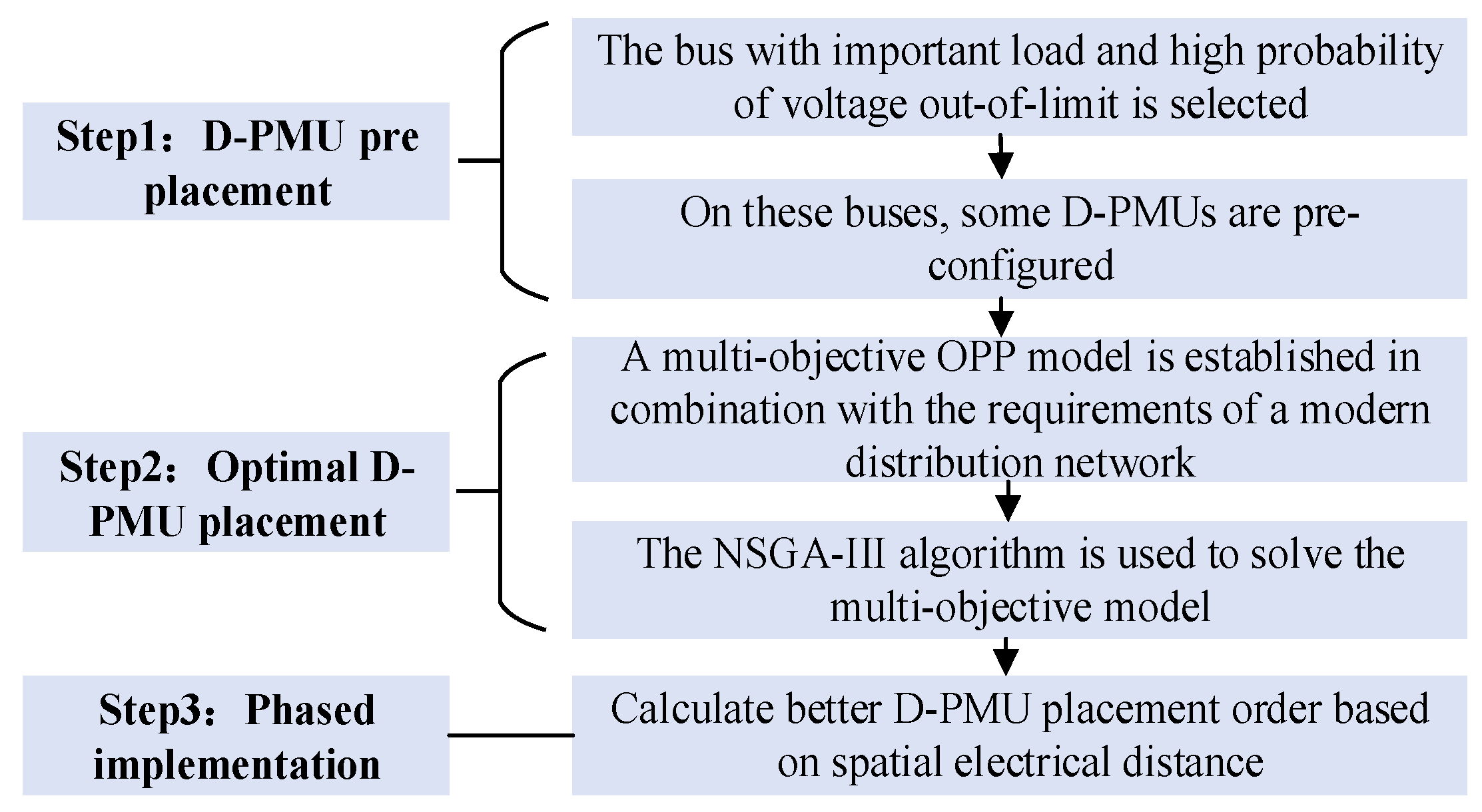
- (1)
- An overall placement process of distribution network D-PMU is presented, which includes initial placement, overall placement and multistage placement.
- (2)
- A topology generation method is proposed, which takes both the current and future economic reconfigurations of distribution networks into account.
- (3)
- A multi-objective optimal D-PMU placement model considering topology changes and contingencies is proposed. The proposed model takes both zero-injection buses and other measurements into account, which not only minimizes the number of D-PMUs, but it also maximizes the ANOBC and NMR under the topology observability constraint. Compared with other methods, the proposed method can greatly reduce the D-PMU number with a high ANOBC and NMR.
- (4)
- The NSGA-III algorithm gives the Pareto optimization solution set of the model. In addition, The Technique for Order Preference by Similarity to an Ideal Solution (TOPSIS) method is applied to select the optimal compromise solution.
- (5)
- The placement order calculation method based on spatial electric distance is proposed, which can provide the D-PMU placement in order to improve the state estimation effect faster.
2. The Overall Strategy of D-PMU Placement
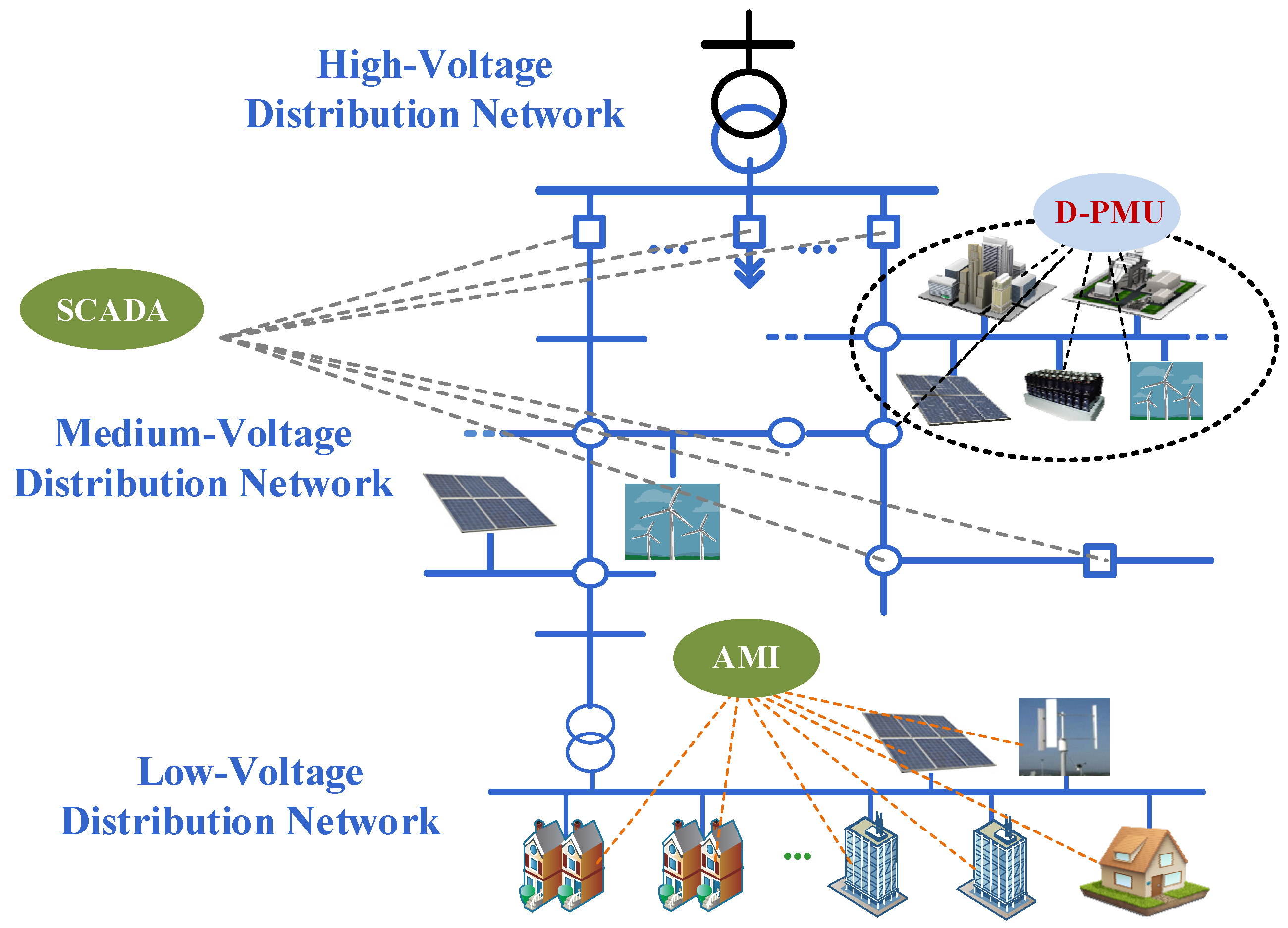
2.1. The Overall Strategy of D-PMU Placement in Distribution Network
2.2. Initial Placement of D-PMU
2.3. Analysis of the Observability
- (1)
- If a D-PMU is placed on a bus, this bus and its neighbors are observable, because for a bus with a D-PMU, the voltage phasor and current phasor of the associated branches are known, and the voltage phasors of its neighbors can be calculated by the Kirchhoff laws;
- (2)
- If a ZIB is observable, and if only one neighbor’s observability is unknown, the voltage phasor of this unknown neighbor can be calculated by the Kirchhoff laws. In other words, this neighbor is identified as observable;
- (3)
- If all neighbors of a ZIB are observable, the voltage phasor of the ZIB can be calculated by the Kirchhoff laws.
3. Multi-Objective OPP Model
3.1. The First Objective Function Considering Economic Factors
3.2. The Second Objective Function Considering ANOBC
3.2.1. Line N-1 Contingencies and D-PMU N-1 Contingencies
- (1)
- Bus i has a D-PMU;
- (2)
- At least two buses in set P1 have a D-PMU;
- (3)
- At least one bus in set P2 has a D-PMU.
- (1)
- Bus i has a D-PMU, and set P has at least one D-PMU;
- (2)
- At least two buses in set P have a D-PMU.
3.2.2. Number of Observable Buses under D-PMU N-1 Contingencies
3.2.3. Impact of ZIB and SCADA
3.2.4. Observability of Non-Critical Bus Based on AMI Data
3.3. The Third Objective Function Considering NMR
3.4. The Constraints Considering the Network Observability
3.5. Multi-Objective OPP Model Considering Topology Changes
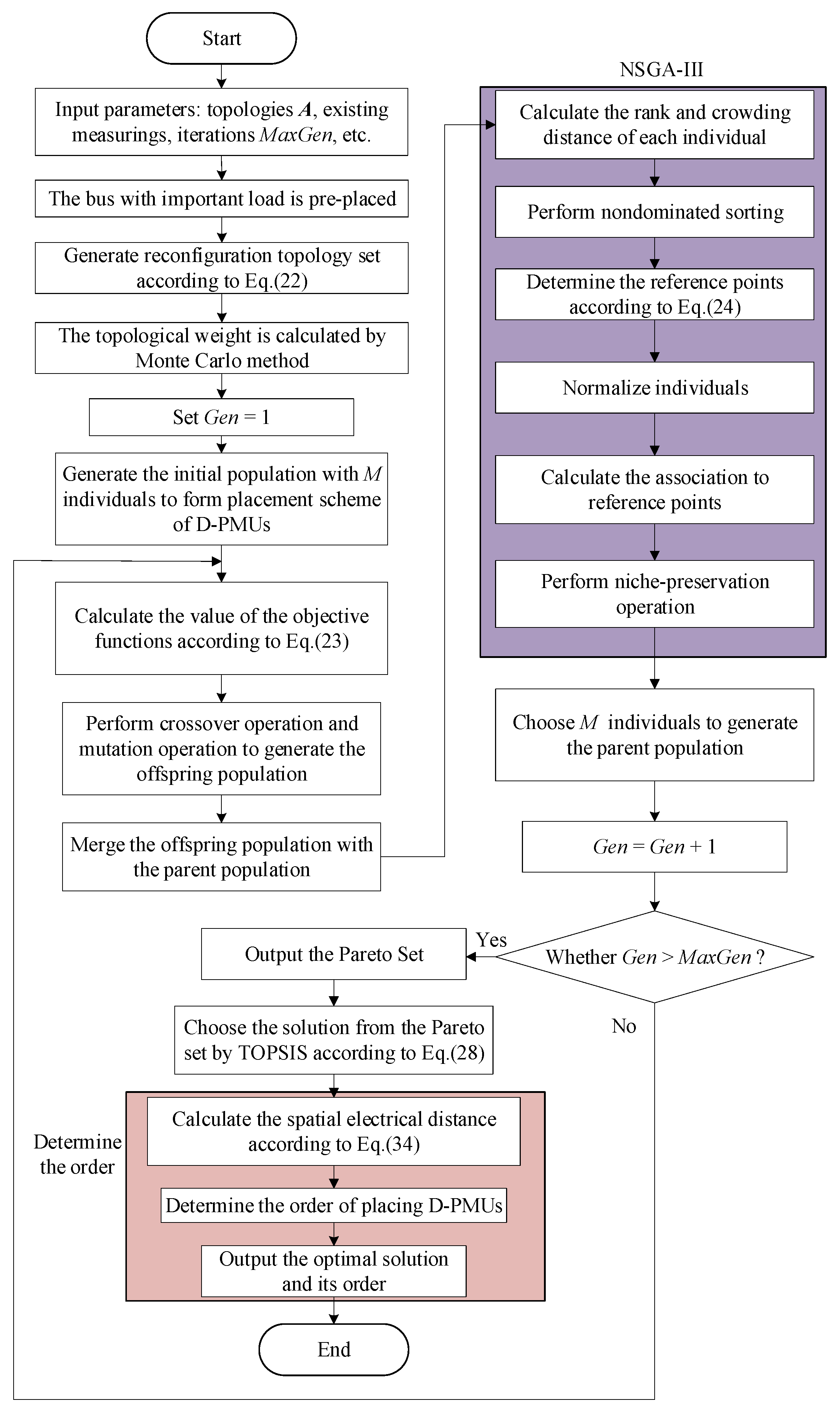
3.6. Solution Methodology Based on NSGA-III
4. D-PMU Placement Order Determination Based on Spatial Electrical Distance
4.1. Spatial Electrical Distance
4.2. Determining the Order of D-PMUs
- (1)
- All buses in the optimal solution that need to be installed with D-PMU are combined into a candidate set;
- (2)
- For each bus in the candidate set, all newly added observable buses should be found after the given bus has been assigned a D-PMU;
- (3)
- By summing the associated weights of the bus with those of the newly added observable buses, the integrated weight is obtained;
- (4)
- The bus with the largest value of is chosen as the next location for installing the D-PMU. Then, this bus is removed from the candidate set;
- (5)
- Is the candidate set empty? If the answer is yes, end. If the answer is no, go to step 2.
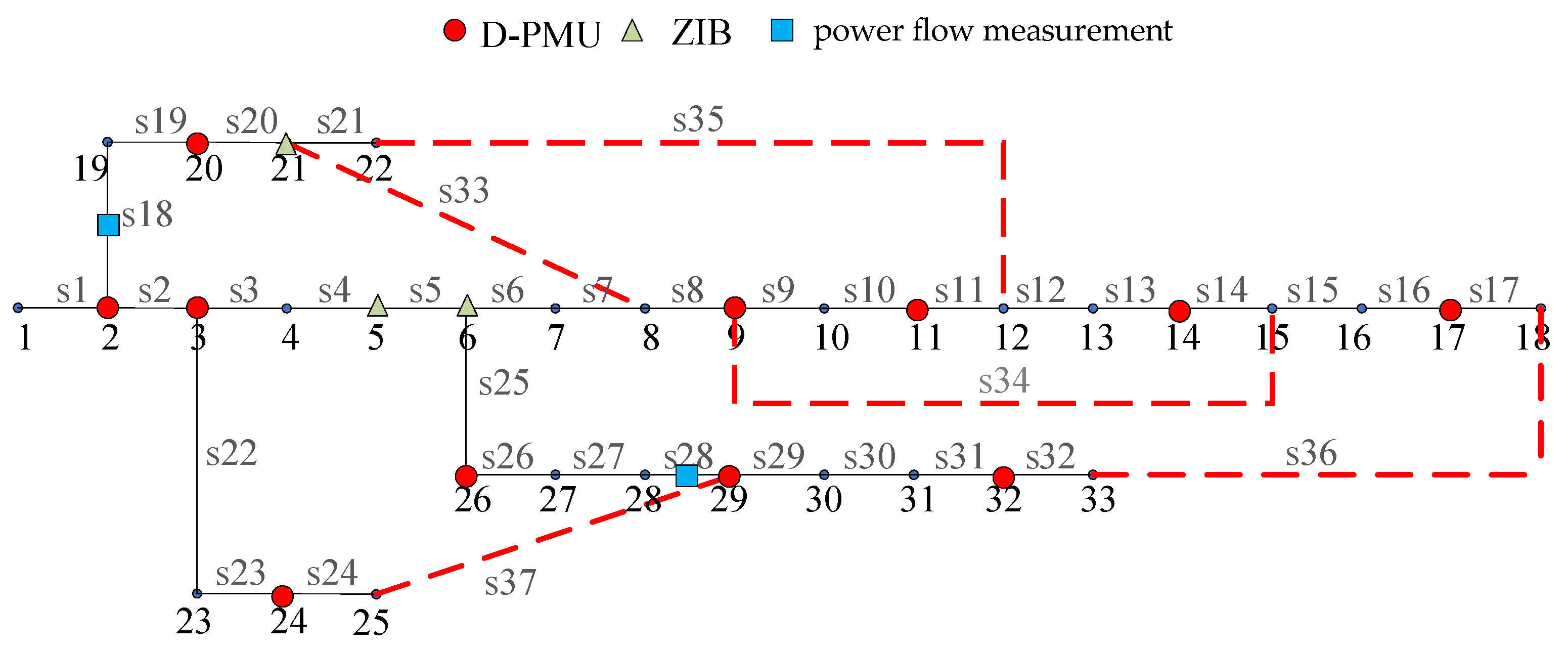
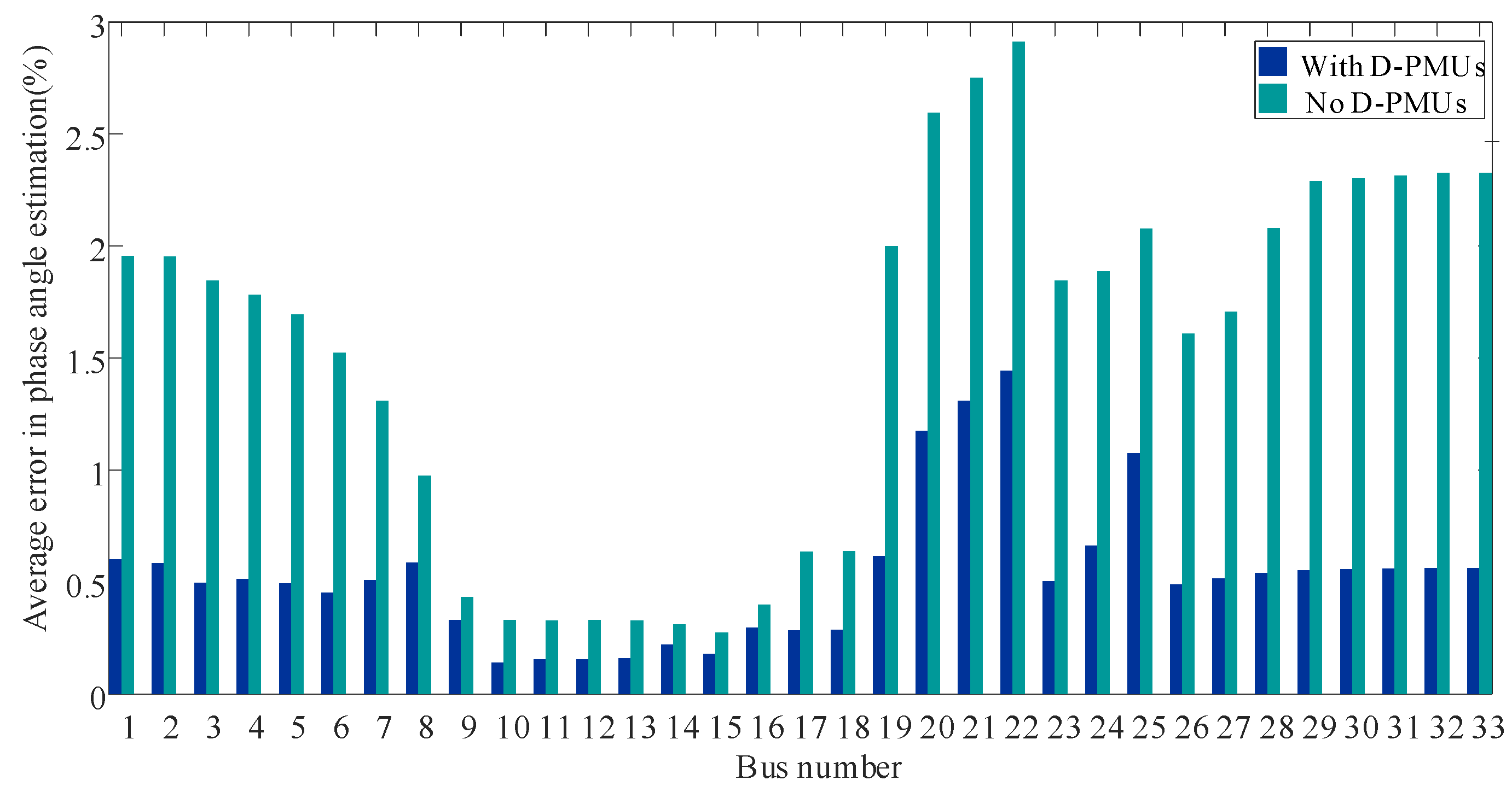
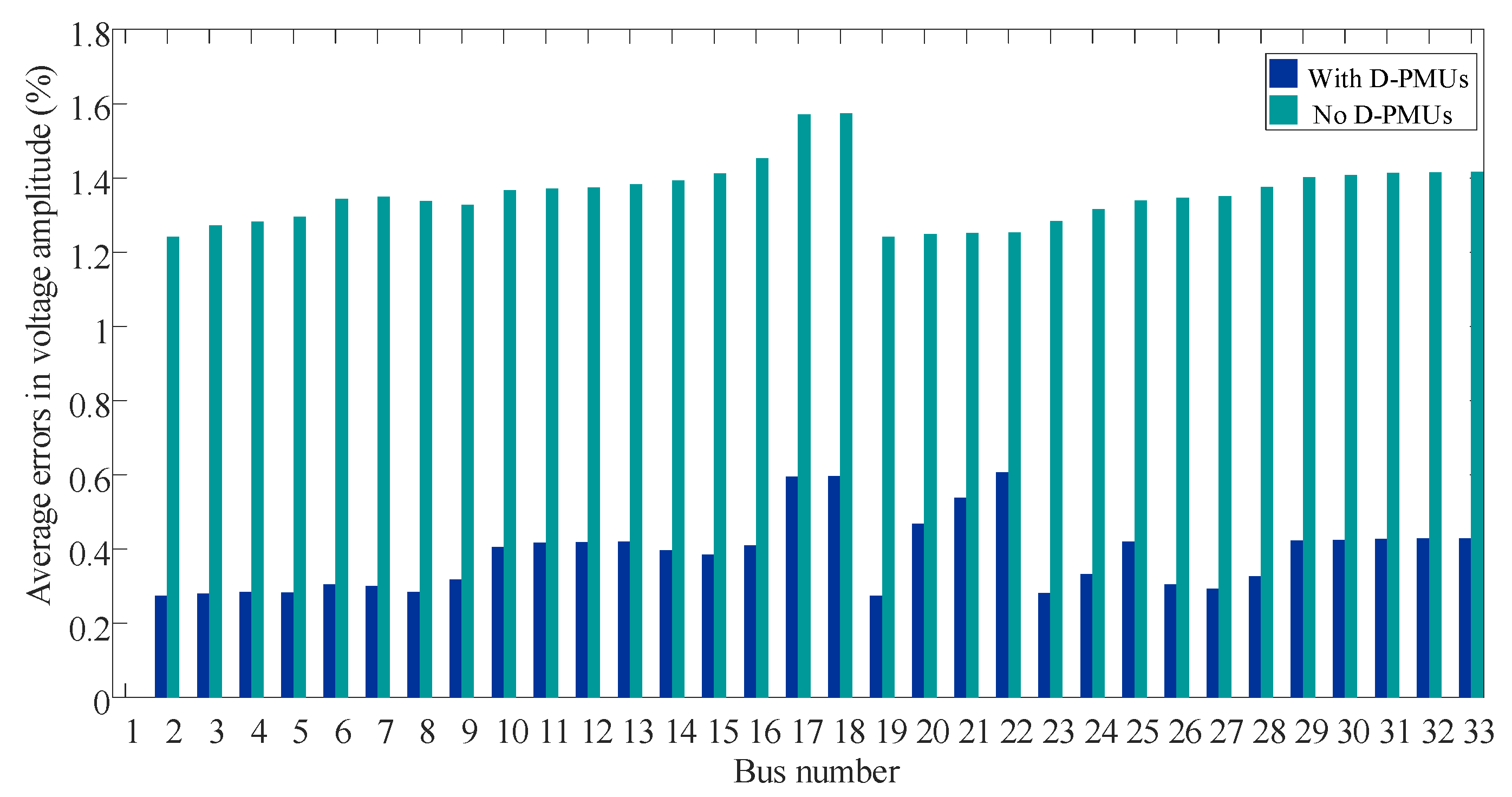
5. Simulation Results
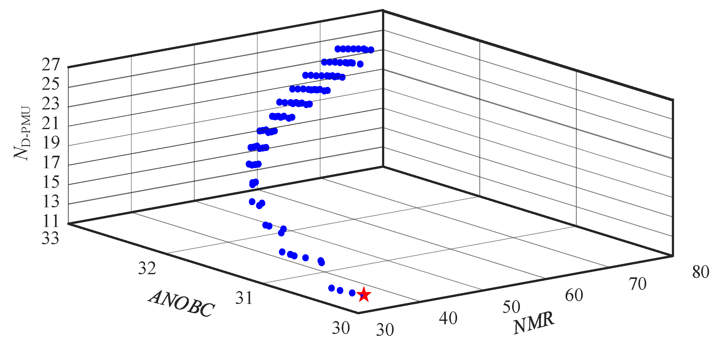
5.1. The Pareto Solution Set Based on NSGA-III
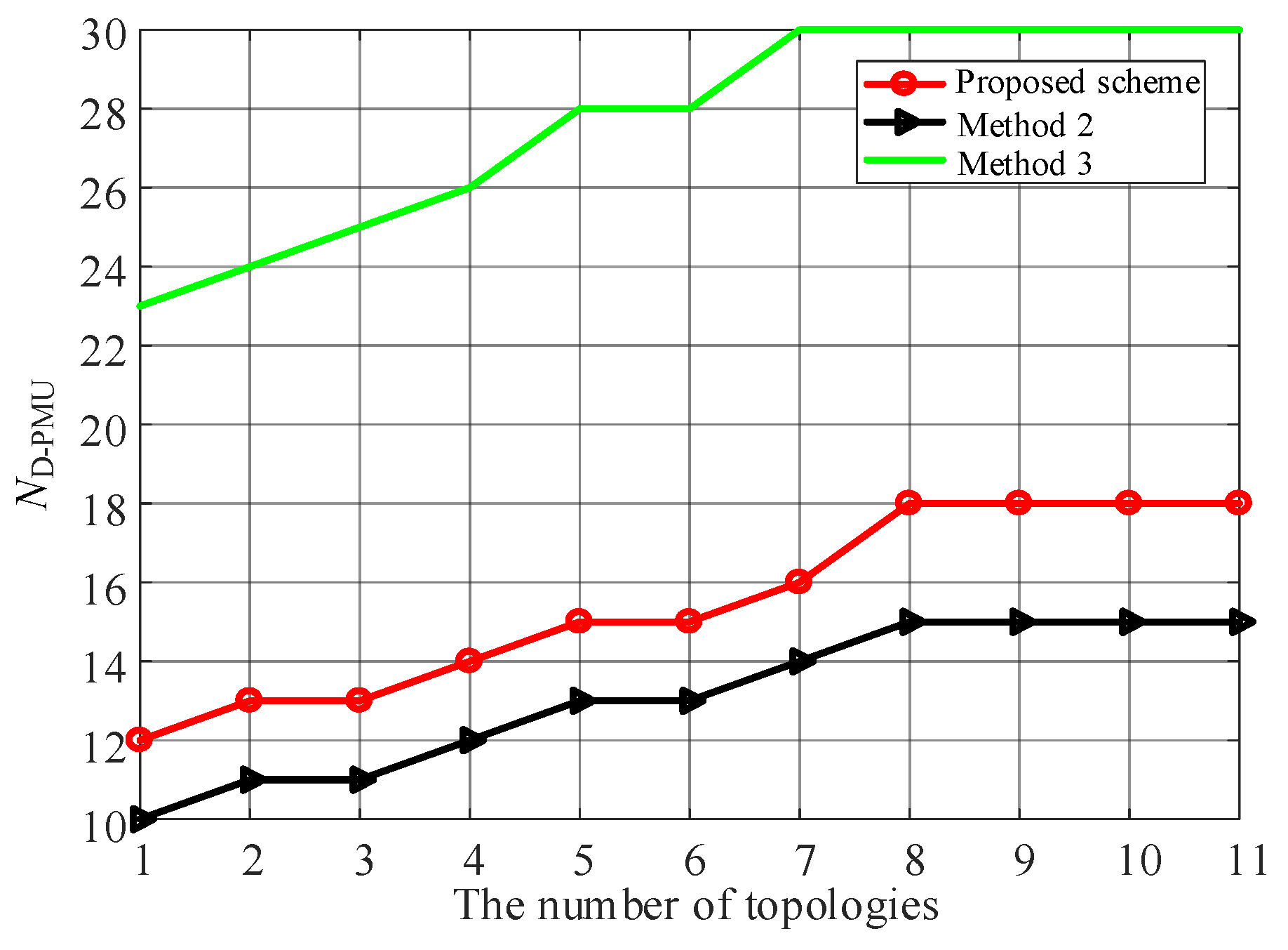
5.2. Method Comparison
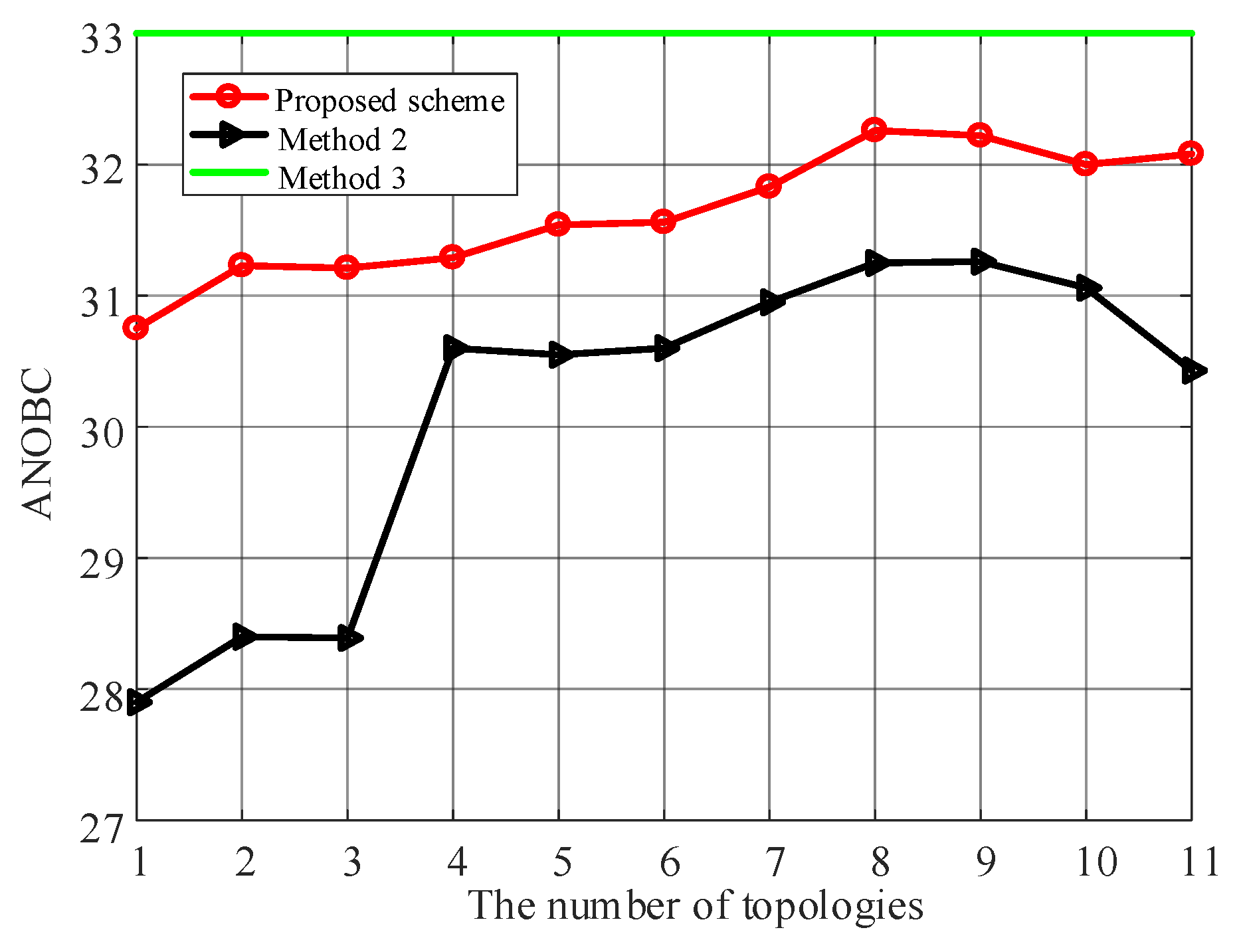
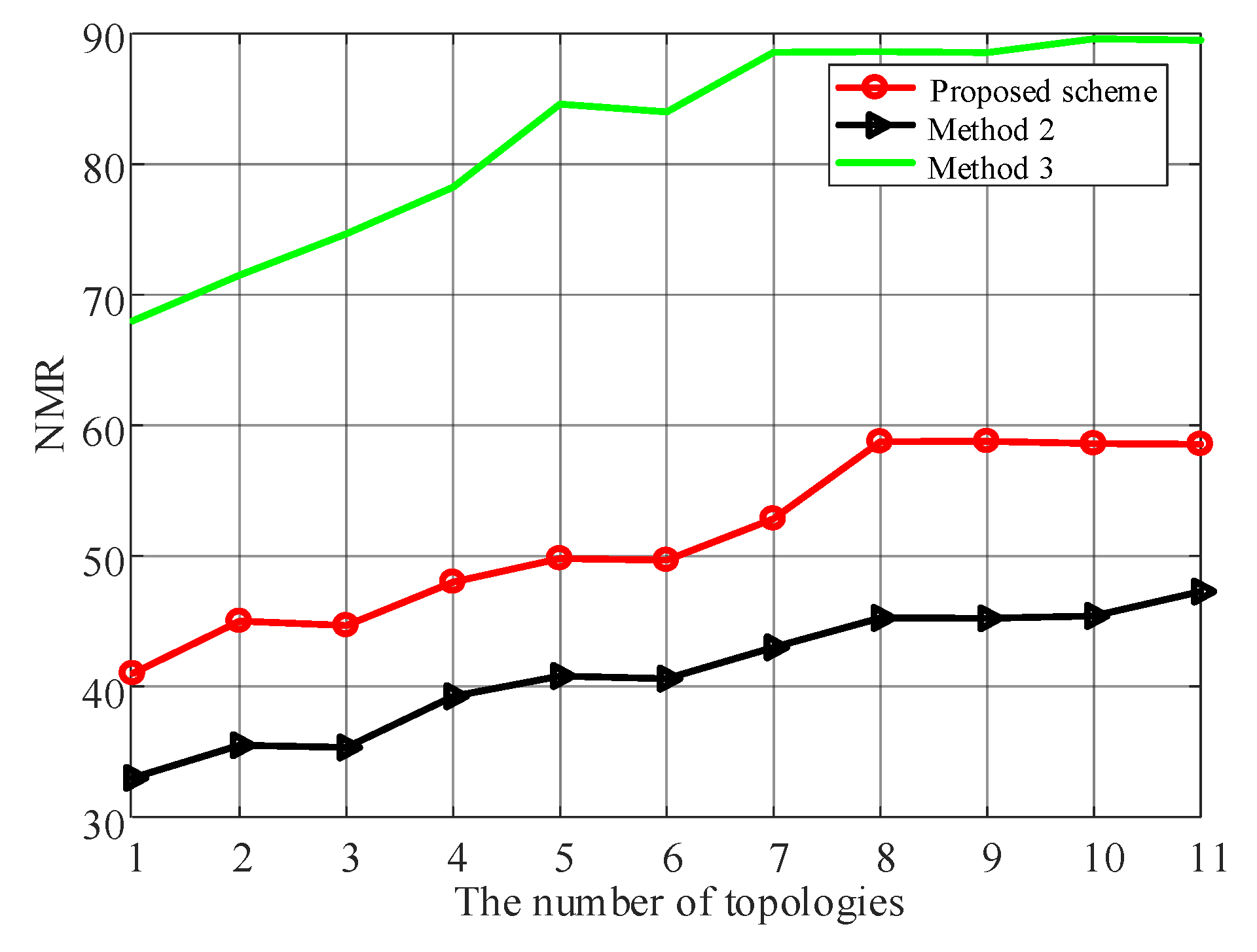
5.3. The Influence of Topology Number
6. Conclusions
Author Contributions
Funding
Institutional Review Board Statement
Informed Consent Statement
Data Availability Statement
Conflicts of Interest
Appendix A


References
- Kong, X.; Xu, Y.; Jiao, Z.; Dong, D.; Yuan, X.; Li, S. Fault Location Technology for Power System Based on Information about the Power Internet of Things. IEEE Trans. Ind. Inform. 2020, 16, 6682–6692. [Google Scholar] [CrossRef]
- Ahmed, M.M.; Amjad, M.; Qureshi, M.A.; Imran, K.; Haider, Z.M.; Khan, M.O. A Critical Review of State-of-the-Art Optimal PMU Placement Techniques. Energies 2022, 15, 2125. [Google Scholar] [CrossRef]
- Joshi, P.M.; Verma, H.K. Synchrophasor measurement applications and optimal D-PMU placement: A review. Electr. Power Syst. Res. 2021, 199, 107428. [Google Scholar] [CrossRef]
- Lambrou, C.; Mandoulidis, P.; Vournas, C. Validation of Voltage Instability Detection and Control Using a Real Power System Incident. Energies 2021, 14, 7165. [Google Scholar] [CrossRef]
- Lee, K.-Y.; Park, J.-S.; Kim, Y.-S. Optimal Placement of D-PMU to Enhance Supervised Learning-Based Pseudo-Measurement Modelling Accuracy in Distribution Network. Energies 2021, 14, 7767. [Google Scholar] [CrossRef]
- Chauhan, K.; Sodhi, R. Placement of Distribution-Level Phasor Measurements for Topological Observability and Monitoring of Active Distribution Networks. IEEE Trans. Instrum. Meas. 2019, 69, 3451–3460. [Google Scholar] [CrossRef]
- Almasabi, S.; Mitra, J. Multistage Optimal D-PMU Placement Considering Substation Infrastructure. IEEE Trans. Ind. Appl. 2018, 54, 6519–6528. [Google Scholar] [CrossRef]
- Khorram, E.; Jelodar, M.T. D-PMU placement considering various arrangements of lines connections at complex buses. Int. J. Electr. Power Energy Syst. 2018, 94, 97–103. [Google Scholar] [CrossRef]
- Kumar, S.; Tyagi, B.; Kumar, V.; Chohan, S. Optimization of Phasor Measurement Units Placement Under Contingency Using Reliability of Network Components. IEEE Trans. Instrum. Meas. 2020, 69, 9893–9906. [Google Scholar] [CrossRef]
- Kong, X.; Wang, Y.; Yuan, X.; Yu, L. Multi Objective for D-PMU Placement in Compressed Distribution Network Considering Cost and Accuracy of State Estimation. Appl. Sci. 2019, 9, 1515. [Google Scholar] [CrossRef] [Green Version]
- Manousakis, N.M.; Korres, G.N. Optimal Allocation of Phasor Measurement Units Considering Various Contingencies and Measurement Redundancy. IEEE Trans. Ind. Inform. 2020, 69, 3403–3411. [Google Scholar] [CrossRef]
- Chen, T.; Cao, Y.; Chen, X.; Sun, L.; Zhang, J.; Amaratunga, G.A.J. Optimal D-PMU placement approach for power systems considering non-Gaussian measurement noise statistics. Int. J. Electr. Power Energy Syst. 2021, 126, 106577. [Google Scholar] [CrossRef]
- Khajeh, K.G.; Bashar, E.; Rad, A.M.; Gharehpetian, G. Integrated Model Considering Effects of Zero Injection Buses and Conventional Measurements on Optimal D-PMU Placement. IEEE Trans. Smart Grid 2017, 8, 1006–1013. [Google Scholar]
- Manousakis, N.M.; Korres, G.N. Optimal PMU Placement for Numerical Observability Considering Fixed Channel Capacity—A Semidefinite Programming Approach. IEEE Trans. Power Syst. 2016, 31, 3328–3329. [Google Scholar] [CrossRef]
- Wu, Z.; Du, X.; Gu, W.; Liu, Y.; Ling, P. Optimal D-PMU Placement Considering load loss and Relaying in Distribution Networks. IEEE Access 2018, 6, 33645–33653. [Google Scholar] [CrossRef]
- Pei, C.; Xiao, Y.; Liang, W.; Han, X. D-PMU Placement Protection Against Coordinated False Data Injection Attacks in Smart Grid. IEEE Trans. Ind. Appl. 2020, 56, 4381–4393. [Google Scholar] [CrossRef]
- Arpanahi, M.K.; Alhelou, H.H.; Siano, P. A Novel Multiobjective OPP for Power System Small Signal Stability Assessment Considering WAMS Uncertainties. IEEE Trans. Ind. Inform. 2020, 16, 3039–3050. [Google Scholar] [CrossRef]
- Abdolrahim, A.; Khalil, G.F. Optimal D-PMU Placement for Power System Observability Considering Network Expansion and N-1 Contingencies. IET Gener. Transm. Distrib. 2018, 18, 4216–4224. [Google Scholar]
- Zhu, S.; Wu, L.; Mousavian, S.; Roh, J.H. An optimal joint placement of D-PMUs and flow measurements for ensuring power system observability under N-2 transmission contingencies. Int. J. Electr. Power Energy Syst. 2018, 95, 254–265. [Google Scholar] [CrossRef]
- Chen, X.; Wei, F.; Cao, S.; Soh, C.B.; Tseng, K.J. PMU Placement for Measurement Redundancy Distribution Considering Zero Injection Bus and Contingencies. IEEE Syst. J. 2020, 14, 5396–5406. [Google Scholar] [CrossRef]
- Wang, S.; Liu, G.; Huang, R.; Qin, S. State Estimation Method for Active Distribution Networks Under Environment of Hybrid Measurements with Multiple Sampling Periods. Autom. Electron. Power Syst. 2016, 40, 30–36. [Google Scholar]
- Rao, R.S.; Ravindra, K.; Satish, K.; Narasimham, S.V.L. Power Loss Minimization in Distribution System Using Network Reconfiguration in the Presence of Distributed Generation. IEEE Trans. Power Syst. 2013, 28, 317–325. [Google Scholar] [CrossRef]
- Wu, Y.K.; Lee, C.Y.; Liu, L.C.; Tsai, S.H. Study of Reconfiguration for the Distribution System with Distributed Generators. IEEE Trans. Power Deliv. 2010, 25, 1678–1685. [Google Scholar] [CrossRef]
- Nara, K.; Mishima, Y.; Satoh, T. Network reconfiguration for loss minimization and load balancing. In Proceedings of the 2003 IEEE Power Engineering Society General Meeting (IEEE Cat. No. 03CH37491), Toronto, ON, Canada, 13–17 July 2003; pp. 2413–2418. [Google Scholar]
- Baran, M.E.; Wu, F.F. Network reconfiguration in distribution systems for loss reduction and load balancing. IEEE Trans. Power Deliv. 1989, 4, 1401–1407. [Google Scholar] [CrossRef]
- Wang, Y.; Chen, Q.; Zhang, N.; Wang, Y. Conditional Residual Modeling for Probabilistic Load Forecasting. IEEE Trans. Power Syst. 2018, 33, 7327–7330. [Google Scholar] [CrossRef]
- Deb, K.; Jain, H. An Evolutionary Many-Objective Optimization Algorithm Using Reference-Point-Based Nondominated Sorting Approach, Part I: Solving Problems With Box Constraints. IEEE Trans. Evol. Comput. 2014, 18, 577–601. [Google Scholar] [CrossRef]
- Jain, H.; Deb, K. An Evolutionary Many-Objective Optimization Algorithm Using Reference-Point Based Nondominated Sorting Approach, Part II: Handling Constraints and Extending to an Adaptive Approach. IEEE Trans. Evol. Comput. 2014, 18, 602–622. [Google Scholar] [CrossRef]
- Yuan, Y.; Xu, H.; Wang, B.; Yao, X. A New Dominance Relation-Based Evolutionary Algorithm for Many-Objective Optimization. IEEE Trans. Evol. Comput. 2016, 20, 16–37. [Google Scholar] [CrossRef]
- Wang, T.C.; Lee, H.D. Developing a fuzzy TOPSIS approach based on subjective weights and objective weights. Expert Syst. Appl. 2009, 36, 8980–8985. [Google Scholar] [CrossRef]
- Chen, Y.; Kong, X.; Yong, C.; Ma, X.; Yu, L. Distributed State Estimation for Distribution Network with Phasor Measurement Units Information. Energy Procedia 2019, 158, 4129–4134. [Google Scholar] [CrossRef]
- Abdelsalam, H.A.; Abdelaziz, A.Y.; Osama, R.A.; Salem, R.H. Impact of Distribution System Reconfiguration on Optimal Placement of Phasor Measurement Units. In Proceedings of the 2014 Clemson University Power Systems Conference (PSC), Clemson, SC, USA, 11–14 March 2014; pp. 1–6. [Google Scholar]
- Zhou, X.; Sun, H.; Zhang, C.; Dai, Q. Optimal placement of D-PMUs using adaptive genetic algorithm considering measurement redundancy. International Journal of Reliability. Qual. Saf. Eng. 2016, 23, 921–929. [Google Scholar]


| Algorithm | Num. of D-PMUs | ANOBC | NMR | Execution Time/s |
|---|---|---|---|---|
| NSGA-III | 11 | 30.64 | 36.5 | 2.3503 |
| NSGA-II | 11 | 30.36 | 35.5 | 2.6363 |
| NSGA-II (Only consider num) | 11 | 28.68 | 34.5 | 2.3728 |
| Method | IEEE 33-Bus System | IEEE 69-Bus System | ||
|---|---|---|---|---|
| Num | D-PMU Locations | Num | D-PMU Locations | |
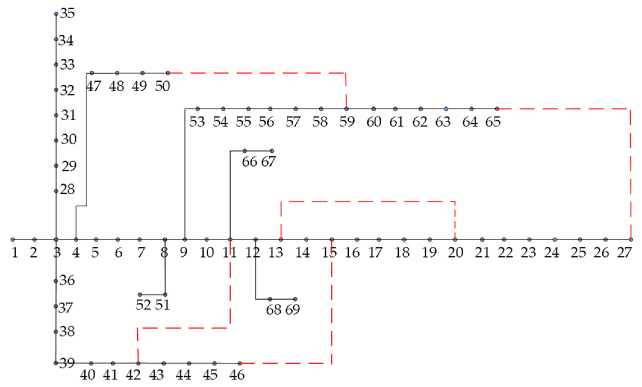
| Proposed Method | 11 | 2, 3, 9, 11, 14, 17, 20, 24, 26, 29, 32 | 24 | 2, 3, 8, 13, 16, 19, 23, 26, 30, 34, 37, 40, 43, 45, 49, 51, 53, 56, 59, 60, 63, 64, 66, 68 |
| Ref. [32] | 14 | 2, 4, 6, 8, 11, 13, 15, 17, 21, 23, 24, 27, 29, 32 | 27 | 1, 4, 5, 8, 9, 12, 15, 18, 20, 23, 26, 29, 32, 34, 37, 40, 42, 45, 49, 52, 53, 55, 58, 61, 64, 66, 69 |
| Ref. [33] | 11 | 2, 6, 8, 11, 15, 17, 21, 24, 28, 29, 32 | 26 | 1, 4, 8, 14, 17, 19, 21, 24, 27, 28, 31, 34, 37, 39, 42, 45, 49, 51, 54, 56, 59, 61, 64, 66, 68, 69 |
| Method | IEEE 33-Bus System | |||
|---|---|---|---|---|
| NMR | Observability of Topology | ANOBC | ||
| Topology 1 | Topology 2 | |||
| Proposed Method | 36.5 | Yes | Yes | 30.64 |
| Ref. [32] | 45.0 | Yes | Yes | 31.64 |
| Ref. [33] | 37.5 | Yes | No | 29.54 |
| Method | IEEE 69-Bus System | |||
|---|---|---|---|---|
| NMR | Observability of Topology | ANOBC | ||
| 1 | 2 | |||
| Proposed Method | 77.5 | Yes | Yes | 62.63 |
| Ref. [32] | 81.0 | Yes | Yes | 65.68 |
| Ref. [33] | 79.0 | Yes | No | 65.07 |
| Topology | IEEE 33-Bus System | |
|---|---|---|
| Closed | Open | |
| 1 | no | no |
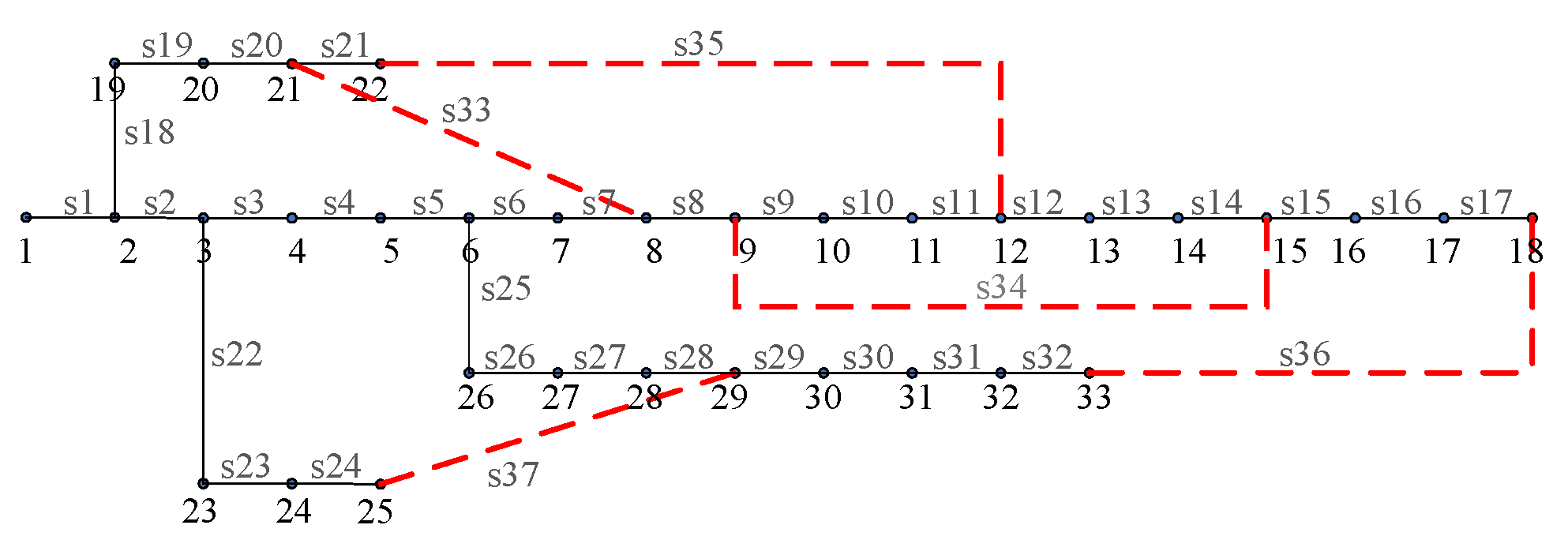
| 2 | s33, s34, s35 | s7, s9, s14 |
| 3 | s35, s37 | s7, s25 |
| 4 | s34, s36 | s13, s17 |
| 5 | s33, s37 | s5, s26 |
| 6 | s36, s37 | s16, s25 |
| 7 | s36, s37 | s24, s31 |
| 8 | s33, s34, s35 | s6, s11, s12 |
| 9 | s34, s36 | s14, s15 |
| 10 | s35, s37 | s2, s3 |
| 11 | s34, s36, s37 | s12, s23, s27 |
Publisher’s Note: MDPI stays neutral with regard to jurisdictional claims in published maps and institutional affiliations. |
© 2022 by the authors. Licensee MDPI, Basel, Switzerland. This article is an open access article distributed under the terms and conditions of the Creative Commons Attribution (CC BY) license (https://creativecommons.org/licenses/by/4.0/).
Share and Cite
Sun, Y.; Hu, W.; Kong, X.; Shen, Y.; Yang, F. Multi-Objective Optimal D-PMU Placement for Fast, Reliable and High-Precision Observations of Active Distribution Networks. Appl. Sci. 2022, 12, 4677. https://doi.org/10.3390/app12094677
Sun Y, Hu W, Kong X, Shen Y, Yang F. Multi-Objective Optimal D-PMU Placement for Fast, Reliable and High-Precision Observations of Active Distribution Networks. Applied Sciences. 2022; 12(9):4677. https://doi.org/10.3390/app12094677
Chicago/Turabian StyleSun, Yuce, Wei Hu, Xiangyu Kong, Yu Shen, and Fan Yang. 2022. "Multi-Objective Optimal D-PMU Placement for Fast, Reliable and High-Precision Observations of Active Distribution Networks" Applied Sciences 12, no. 9: 4677. https://doi.org/10.3390/app12094677